City, University of London Institutional Repository
Citation
:
Castro-Alvaredo, O. and Fring, A. (2001). Constructing infinite particle spectra.
Physical Review D (PRD), 64(8), doi: 10.1103/PhysRevD.64.085005
This is the unspecified version of the paper.
This version of the publication may differ from the final published
version.
Permanent repository link:
http://openaccess.city.ac.uk/721/
Link to published version
:
http://dx.doi.org/10.1103/PhysRevD.64.085005
Copyright and reuse:
City Research Online aims to make research
outputs of City, University of London available to a wider audience.
Copyright and Moral Rights remain with the author(s) and/or copyright
holders. URLs from City Research Online may be freely distributed and
linked to.
City Research Online:
http://openaccess.city.ac.uk/
[email protected]
arXiv:hep-th/0103252v2 9 Apr 2001
Constructing Infinite Particle Spectra
O.A. Castro-Alvaredo and A. Fring
Institut f¨ur Theoretische Physik, Freie Universit¨at Berlin, Arnimallee 14, D-14195 Berlin, Germany
(February 1, 2008)
We propose a general construction principle which allows to include an infinite number of resonance states into a scat-tering matrix of hyperbolic type. As a concrete realization of this mechanism we provide new S-matrices generalizing a class of hyperbolic ones, which are related to a pair of simple Lie algebras, to the elliptic case. For specific choices of the al-gebras we propose elliptic generalizations of affine Toda field theories and the homogeneous sine-Gordon models. For the generalization of the sinh-Gordon model we compute expliitly renormalization group scaling functions by means of the c-theorem and the thermodynamic Bethe ansatz. In particular we identify the Virasoro central charges of the corresponding ultraviolet conformal field theories.
PACS numbers: 11.55.Ds, 11.10.Hi, 11.10.Kk, 05.70.Jk
I. INTRODUCTION
Treating quantum field theories in 1+1 dimensions as a test laboratory for realistic theories in higher dimensions, this paper is concerned with the general question of how to enlarge a given finite particle spectrum of a theory to an infinite one.
In general the bootstrap [1], which is the construction principle for the scattering matrix, is assumed to close after a finite number of steps, which means it involves a finite number of particles. However, from a physical as well as from a mathematical point of view, it ap-pears to be natural to extend the construction in such a way that it would involve an infinite number of parti-cles. The physical motivation for this are string theories, which admit an infinite particle spectrum. Mathemati-cally the infinite bootstrap would be an analogy to infi-nite dimensional groups, in the sense that two entries of the S-matrix are combined into a third, which is again a member of the same infinite set. It appears to us that it is impossible to construct an infinite bootstrap system involving asymptotic states and find the mathematical analogue to infinite groups in this sense (see also foot-note 2 and the paragraph after figure 1). However, it is possible to introduce an infinite number of unstable particles into the spectrum. Scattering matrices which would allow such type of interpretation have occurred in the literature [3–5], although only in the latter paper a reference to unstable particles has been made. In [4,5] these matrices were found to be expressible in terms of elliptic functions, a feature very common in the context of lattice models, e.g. [7]. The main purpose of this paper is to suggest a general construction principle for such type
of S-matrices starting from some known theory with a finite particle spectrum of a special, albeit quite generic, form. As particular examples we provide elliptic gener-alizations of scattering matrices related to a pair of Lie algebras [6], which contain the affine Toda S-matrices [8] and homogeneous sine-Gordon S-matrices [9] for partic-ular choices of the algebras.
Our paper is organized as follows: In section II we provide a general principle for the construction of scat-tering matrices which involve an infinite number of un-stable particles and present some explicit examples. In section III we construct renormalization group (RG) scal-ing functions by means of the c-theorem and the thermo-dynamic Bethe ansatz (TBA) for the generalization of the sinh-Gordon model. Our conclusions and an outlook towards open problems are stated in section IV.
II. CONSTRUCTION PRINCIPLE
Let us consider the huge class of two-particle S-matrices, which describe the scattering between particles of typeaandbas a function of the rapidity differenceθ, of the general form1
Sab(θ) =Sabmin(θ)SabCDD(θ). (1)
Here Smin
ab (θ) denotes the so-called minimal S-matrix
which satisfies the consistency relations [1], namely uni-tarity, crossing and the fusing bootstrap equations and possibly possess poles on the imaginary axis in the sheet 0 ≤ Imθ ≤ π, which is physical for asymptotic states. The CDD-factor [2], referred to as SCDD
ab (θ), also
sat-isfies these equations, but has its poles in the sheet −π≤Imθ≤0, which is the “physical one” for resonance states. SCDD
ab (θ) might depend on additional constants
like the effective coupling constant or a resonance param-eter. A simple prescription to introduce now an infinite number of resonance poles is to replace the CDD-factor in (1) by
ˆ
SabCDD(θ, N) = N
Y
n=−N
SCDDab (θ+nω), (2)
1Exceptions to this factorization are for instance the
where ω is taken to be real. By construction the new S-matrix, ˆSab(θ, N) = Smin
ab (θ) ˆSabCDD(θ, N) satisfies the
bootstrap consistency equations and possible poles in the sheet−π≤Imθ≤0 have now been duplicated 2N times within this sheet, such that they admit an interpretation as unstable particles. Therefore, whenN → ∞we have an infinite number of resonance poles. Since, as a conse-quence of crossing and unitarity, the S-matrix is known to be a 2πi-periodic function, a property shared indi-vidually bySCDD
ab (θ, N), we expect to recover a double
periodic function in the limitN → ∞ lim
N→∞
ˆ
SabCDD(θ, N) = lim
N→∞
ˆ
SabCDD(θ+µ2πi+νω, N) (3)
for µ, ν ∈ Z. At this stage it is not clear whether the prescription (2) is meaningful at all, in the sense that it leads to meaningful quantum field theories, and in par-ticular one has to be concerned about the convergence of the infinite product in (3). Since limN→∞SˆabCDD(θ, N)
is a double periodic function we expect that it is some-how related to elliptic functions (see e.g. [11] for their properties). Let us therefore now look concretely at the building blocks which can be used to make up the entire scattering matrix in the non-elliptic case, when backscat-tering is absent. In that case the S-matrices are diagonal and known [12] to be of the general form
Sab(θ) = Y
x∈A
{x}σ
θ =
Y
x∈A
tanh(θ−iπx+σ)/2 tanh(θ+iπx+σ)/2, (4) with x∈ Qand σ ∈R. A specific theory is then char-acterized by the finite setA2. This means, if we
demon-strate that the prescription (3) is meaningful for each individual building block{x}σ
θ as defined in (4), in
par-ticular we need to demonstrate the convergence of the infinite product, we have established that it is sensible for the entire scattering matrix. For this purpose we note the identity
{x}σ
θ,ℓ:=
∞
Y
n=−∞
{x}σ
θ+nω=
scθ−dnθ+
scθ+dnθ−
. (5)
Here we abbreviatedθ± = (θ±iπx+σ)iKℓ/πand used
the Jacobian elliptic functions in the standard notation pq(z) with p,q ∈ {s,c,d,n} (see e.g. [11]). The quarter periods Kℓ depending on the parameter ℓ ∈ [0,1] are defined in the usual way through the complete elliptic integral
Kℓ=
Z π/2
0
(1−ℓsin2θ)−1/2dθ . (6)
2The fact that x ∈ Q together with the bootstrap leads
to a finite setAand therefore a finite number of asymptotic states. Taking insteadx∈Rcould possibly lead to an infinite number, but a consistent closure of the bootstrap is not known up to now.
The period of {x}σ
θ,ℓ is chosen to be ω = πK(1−ℓ)/Kℓ.
The last identity in (5) is easily derived from the infinite product representations of the elliptic functions which can be found in various places as for instance in [11]
scx=ktan πx 2Kℓ
∞
Y
n=1
1−2q2ncos(πx/Kℓ) +q4n
1 + 2q2ncos(πx/Kℓ) +q4n, (7)
dnx=k−1
∞
Y
n=1
1 + 2q2n−1cos(πx/Kℓ) +q4n−2
1−2q2n−1cos(πx/Kℓ) +q4n−2 , (8)
withk= (1−ℓ)−1/4andq= exp(−ω). Recalling the well
known limits limℓ→0Kℓ =π/2 and limℓ→0K(1−ℓ) =∞
we obtain
lim
ℓ→0{x}
σ
θ,ℓ={x}σθ. (9)
This means in the limitℓ→0 the elliptic S-matrix ˆSab(θ) collapses to the hyperbolic one, that is Sab(θ). Notice that due to the general identity pr(x)/qr(x) = pq(x), we could also write (5) in terms of various other combina-tions of elliptic funccombina-tions. For instance replacing sc by sn/cn is probably most intuitive, since it allows an alter-native prescription to (3) for the construction of elliptic scattering matrices: Replace sinh→sn, cosh→cn and correct the consistency equations by a factor dn, which reduces always to 1 in the hyperbolic limit, in such a way that no resonance poles are left inside the physical sheet. Defining now the function
θµ,ν(x, σ, ω) := 2πi(ν+x/2) + 2ωµ−σ (10) the singularities of{x}σ
θ,ℓare easily identified as
zeros : θµ,ν(x, σ, ω), θµ,ν(1−x, σ, ω), (11) poles : θµ,ν(−x, σ, ω), θµ,ν(x−1, σ, ω). (12) Note that when taking 0≤x≤1 the poles are situated in the non-physical sheet.
This brings us to the question of how to interpret these poles and how can we characterize the physical properties of the related particles? Considering the S-matrixSab(θ), which describes the scattering of two particles of type
aand b with masses ma and mb, we assume that there is a resonance pole situated atθR =σ−iσ¯. According to the Breit-Wigner formula [17] (see also e.g. [18]) the massM˜c and the decay width Γ˜c of an unstable particle
of type ˜c can be conveniently expressed as 2M˜c2=
p
γ2+ ˜γ2+γ, Γ2 ˜
c/2 =
p
γ2+ ˜γ2−γ, (13)
where
γ=m2a+m2b+ 2mambcoshσcos ¯σ, (14)
˜
requires additional investigation. This caution is based on various facts. First, the relations (13) are simply de-rived by carrying over a prescription from usual quantum mechanics to quantum field theory, i.e. complexifying the mass of a stable particle. Second, solving the Breit-Wigner formula for the quantities M˜c, Γc˜ and treating
them literally as mass and decay width is somewhat prob-lematic since this is in conflict with Heisenberg’s uncer-tainty principle, because apparently we know simultane-ously the energy and the time. Third, the Breit-Wigner relations presume an exponential decay in momentum space, which is in fact incompatible with the general principles of quantum field theory and therefore might possibly be a problem in this context [19]. Nonetheless, we employ these quantities and try to find evidence to support that they are indeed meaningful. When taking
M˜c to be the mass of the unstable particle there should
be a threshold for energetic reasons of the type
Mc˜≥ma+mb, (16)
with the consequence that the decay width is bounded by
Γ2c˜≥8mamb(1−coshσcos ¯σ). (17)
So far evidence for these thresholds has not been found in the literature. One reason for this is that the unstable particles enter the bootstrap principle in a more passive way than the stable particles, whose properties are di-rectly used in the construction procedure. Hence one expects that signs for these thresholds will emerge in a more indirect way.
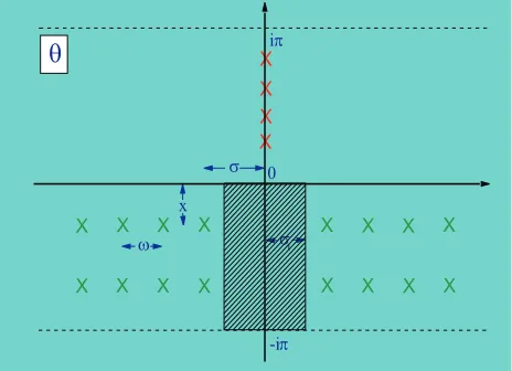
[image:4.612.61.293.460.628.2]A summary of our statements about the pole structure of ˆS(θ) is depicted in figure 1.
Figure 1: The poles of the blocks{x}σ
θ,ℓare the crosses in the
sheet−π≤Imθ≤0. The crosses on the positive part of the imaginary axis are associated, as usual, with stable particles. For equal masses of the stable particles the threshold (16) is
σt= arccosh[(3−cosπx)/(1 + cosπx)].
Since the poles inside the sheet 0 ≤Imθ ≤π are as-sociated toSmin
ab (θ), it is also obvious from figure 1 why
the prescription (2) may not be employed for this part of the S-matrix, since it would lead to a pole structure which is, according to (13), non physical forM˜c and Γ˜c.
A. Examples
It is clear by construction that our prescription in-cludes all affine Toda field theories related to simply laced Lie algebras, since they all factorize as (1) and may be represented in the form (4), see e.g. [8]. Taking the res-onance parameterσ to be zero and the setA={t} for 0≤t≤1, we recover as a special case the elliptic version of the sinh-Gordon model proposed in [5]. Reintroducing
σ, its scattering matrix reads
ˆ
S(θ) =
∞
Y
n=−∞
tanh(θ−iπx+nω+σ)/2
tanh(θ+iπx+nω+σ)/2. (18) According to (13) the masses and decay width of the unstable particles are
Mµ,νσ,nω=m
√
2 coshθµ,ν(y, σ, nω)
2 , y=−x, x−1 (19) Γσ,nωµ,ν =m2
√
2 sinhθµ,ν(y, σ, nω)
2 , y=−x, x−1 (20) where m denotes the mass of the stable particle. The thresholds (16) and (17) translate in this case into
cosh(nω+σ)≥31∓cosπx
±cosπx,Γ≥4m
sin2π(2x+14 ±1) cosπ(2x+14 ±1) .
(21)
As a further example we consider the elliptic general-ization of theA1|AN−1-theory (≡SU(N)2-homogeneous
sine-Gordon model). The two-particle S-matrix describ-ing the scatterdescrib-ing of two stable particles of typeaandb, with 1≤a, b≤N−1, related to the non-elliptic version of this model was proposed in [9]. In our notation it may be written as
Sab(θ, σab) = (−1)δab
caq{1/2}σab
θ
Iab
. (22)
Here I denotes the incidence matrix of the SU(N )-Dynkin diagram, the resonance parameters have the propertyσab=−σbaandca=±1 depending on whether
ais even or odd. According to our prescription outlined in the previous paragraph, the elliptic generalization of (22) is
ˆ
Sab(θ, σab, ℓ) = (−1)δab h
caq{1/2}σab
θ,ℓ
iIab
. (23) Note that despite the appearance of the square root,S
III. RG-SCALING FUNCTIONS
Having established that our prescription leads to sen-sible solutions of the bootstrap consistency equations, we would also like to know what kind of quantum field the-ories these scattering matrices correspond to. Up to now all known solutions to the on-shell consistency equations have led to sensible QFT’s, albeit a rigorous proof which would establish that indeedallsolutions are well-defined local QFT’s is still an outstanding issue. Some crucial characteristics of the theory are contained in the renor-malization group scaling functions, which we now want to determine. In particular, we want to identify in the extreme ultraviolet limit the Virasoro central charges of the corresponding conformal field theories.
A. The c-theorem
We carry out this task by evaluating the c-theorem [14] in the version presented in [13]
c(r) = 3
∞
X
n=1
X
µ1...µn
∞
Z
−∞
dθ1. . . dθn
n!(2π)n e
−r E (24)
× F
Θ|µ1...µn
n (θ1, . . . , θn)
2(6 + 6rE+ 3r2E2+r3E3)
2E4 .
The sum of the on-shell energies is here denoted by
E=Pn
i=1mµicoshθi, withmµi being the masses of the
theory and the correlation function for the trace of the energy momentum tensor Θ has been expanded in terms of n-particle form factorsFΘ|µ1...µn
n (θ1, . . . , θn) (see [20]
for general properties and [16] for explicit sinh-Gordon formulae). We normalized Θ and mµi by an overall
mass scale, such that E as well as the renormalization group parameterr become dimensionless. In particular limr→0c(r) is the ultraviolet Virasoro central charge.
Let us now start with the evaluation ofc(r) as defined in (24) for the elliptic version of the sinh-Gordon model. As the input for this we need to know then-particle form factors. Since so far it is not known how to compute the sum in n analytically, we have to resort to a numerical treatment and it is clear that we have to terminate the series at a certain value of n. Fortunately, it was ob-served explicitly in [16], that in fact the expression for
n = 2 is already very close to the exact answer for the sinh-Gordon model. We assume here that the conver-gence behaviour is still true when we generalize the scat-tering matrix to (18). Note that in general one has to be careful with this approximation, since the higher parti-cle contributions are crucial in some models in order to obtain a good approximation to c(r) [21,13,22]. In the two-particle approximation, indicated by the superscript, one can perform one of the integrations analytically and (24) acquires the simple form
lim
r→0c
(2)(r) = 3
2
∞
Z
0
dθ|F
Θ 2 (2θ)|2
cosh4θ . (25)
It is here crucial to note that besides the formulation of ˆS in terms of elliptic functions for N → ∞, it can also be expressed equivalently in terms of the usual sinh-Gordon S-matrix (5). When trying to solve now the form factor consistency equations [20], we can exploit this ob-servation. Since for the model at hand there is neither a kinematic nor a bound state pole in FΘ
2 (θ), the only
equations to be solved are Watson’s equations. The two particle form factor is then easily obtained to be
ˆ
F2Θ(θ, N) = 2π
N
Y
n=−N
Fmin(θ+nω)
Fmin(iπ+nω)
, (26)
where Fmin(θ) is the minimal form factor of the
sinh-Gordon model obtained in [16]
Fmin(θ) = exp
4 ∞ Z 0 dt t cos tθ π
cotht+isin
tθ
π
× sinh(
t(x−1)
2 ) sinh(
tx
2) sinh(
t
2)
sinh(t)
#
. (27)
Using the infinite product representation forFmin(θ) [16]
the solution (26) forN→ ∞coincides with the equation (5.3) in [5]. Proceeding now to the evaluation of (24), we require|FˆΘ
2 (θ, N)|2, whose characteristics are captured
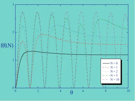
[image:5.612.325.556.431.603.2]in figure 2.
Figure 2: Absolute value squared of the two particle form fac-torsf(θ, N) = |FˆΘ
2 (θ, N)/2π|2 as functions of the rapidity
for different values ofN forω= 1.3 andx= 0.1.
always has a distinct maximum, which we refer to asθm. From (27) follows that it is determined by the solution of
4θm
π coshθmsinπx+ cosh 2xπcoth θm
2
= cosh
3θm
2
sinhθm
2
+ 2(2x−1) cosπxsinhθm. (28)
Solving this equation for various values ofx, we find that
[image:6.612.323.557.238.406.2]θmis always slightly greater than the smallest threshold bound obtained from (21). For instance for x= 0.1 we obtainθm ≃1.439 and nω+σ >0.315 and forx= 0.5 we have θm ≃2.040 and nω+σ >1.763. We interpret this as an indication that the form factors “know” about the thresholds (21). We support this now by considering limN→∞ f(θ, N) for various values ofω.
Figure 3: Absolute value squared of minimal form factors
g(θ, ω) = limN→∞|Fˆmin(θ, N)|2as functions of the rapidity
for different values ofωandx= 0.1.
Figure 4: Integrand of equation (25), that is h(θ, ω) = limN→∞|Fˆmin(θ, N)|2/cosh4θas a function of the rapidity
for different values ofωandx= 0.1.
We observe that in the region in which the factor 1/cosh4(θ), emerging in (25), is still non vanishing the integrals limN→∞R dθ|Fˆmin(θ, N)|2are decreasing
func-tions of ω. This behaviour is changed once we take
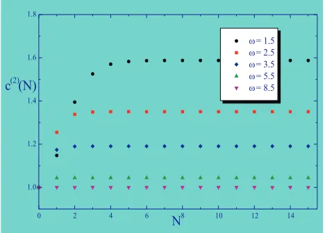
ω < θm as we can explicitly extract from figure 4. Naturally this features are also reflected in the scaling functions. Presuming that for each value ofN we have a consistent theory, we would like to know which ultravio-let central charges these models possess and in addition we want to identify a value ofN for which the related model constitutes reasonably good approximation for the elliptic models. That such an identification is possible is exhibited in figure 5. In addition we observe, that for fixedωandxthe scaling function is a monotonically in-creasing whenN is varied.
Figure 5: Ultraviolet Virasoro central chargec(2)as a function
ofN.
[image:6.612.60.292.252.424.2]Focussing now on the elliptic case, that is we select a large enoughN such that this case is well approximated, we compute the scaling function in dependence ofω for various values ofr. Our results are depicted in figure 6.
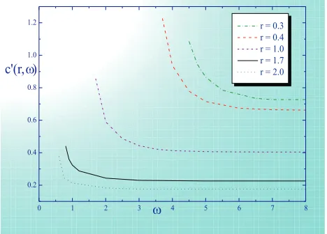
Figure 6: Ultraviolet Virasoro central chargec(2)as a function
[image:6.612.61.291.493.664.2] [image:6.612.323.556.507.676.2]In the extreme limits we obtain limω→0 c(r, ω) =
0 and for large ω we recover the values of the sinh-Gordon model, limω→∞c(r, ω) = cSG(r). The latter
limit follows from (9) and is in addition compatible with limθ→∞Fmin(θ) = 1. The values for the extremal points
were already quoted in [5], however, we also observe that the function is not monotonically increasing between these points as claimed in there. In fact, in the physi-cal region, that is for values ofω >0.315,the function is monotonically decreasing and does not take on values be-tween 0 and 1. Remarkably, the threshold is quite clearly exhibited by a drastic change in the behaviour ofc, that is the onset of a small plateau as is visible in figure 6. We performed the same computation for different values ofxand observed that this onset moves in the direction predicted by equation (21).
B. The thermodynamic Bethe ansatz
Let us now compare the results of the previous section with an alternative method, namely the thermodynamic Bethe ansatz [15]. For this we first have to solve the TBA-equations
rmiˆ coshθ+ ln(1−e−Li(θ)
) =X
j
ϕij∗Lj(θ) (29)
for the function Li(θ). The information of the scat-tering matrix is captured in the kernel ϕij(θ) = −idlnSij(θ)/dθof the rapidity convolution, which is de-noted as usual by f ∗g(θ) := R
dθ′/2π f(θ −θ′)g(θ′).
The dimensionless parameter r =m1T−1 is the inverse
temperatureT times the overall mass scale of the light-est particle m1. Also all masses have been normalized
in this way, i.e. ˆmi =mi/m1. Having determined the
Li(θ)-functions, we may compute the scaling function by means of
c′(r) = 3r
π2
X
i
ˆ
mi
Z ∞
0
dθcoshθ Li(θ) . (30)
Once again limr→0c′(r) is the ultraviolet Virasoro central
charge. We would like to recall here that the scaling functions c(r) and c′(r) are not identical, but contain
qualitatively the same information in the RG sense. In order to carry out this analysis we need to know in (29) the kernel ϕ(θ) as input. For the model under consideration we can exploit the factorization property (18) for a finite product and trivially obtain
ϕN(θ) =
N
X
n=−N
ϕSG(θ+nω+σ), (31)
whereϕSG(θ) is the sinh-Gordon kernel, e.g. [23]
ϕSG(θ) =
4 sin(πx) coshθ
cosh(2θ)−cos(2πx). (32)
Using alternatively the representation of the S-matrix (18) in terms of elliptic functions, we compute the kernel directly to
lim
N→∞ϕN(θ) =
Kℓ π
X
k=−,+
dcθk
snθk +ℓ(1−ℓ)
snθk
dcθk
. (33)
With these expression we carry out our numerical anal-ysis, that is we solve iteratively the equation (29) and evaluate (30) thereafter. The results of this investiga-tions are presented in figure 7.
[image:7.612.323.557.284.452.2]Unfortunately for very small values ofωandrour nu-merical iteration procedure does not converge reliably. However, we will be content at this stage with the data obtained so far, since they already support qualitative our c-theorem analysis. They confirm that above thresh-old the scaling function is monotonically decreasing as a function ofω and also that values greater than 1 may be reached, even for finite values ofr.
Figure 7: TBA scaling function.
IV. CONCLUSIONS
Starting from a given scattering matrix of hyperbolic type, we have demonstrated that it is possible to include consistently an arbitrary number of unstable particles into the spectrum of the theory. In particular when this number becomes infinite the S-matrix may be expressed in terms of elliptic functions.
Concerning the investigation of the c-theorem, it would be desirable to refine the analysis. In particular one should include higher n-particle form factors into the expansion. For the elliptic version some of them were already presented in [5], but in general it remains a challenge to find closed expressions for arbitrary particle numbers. At present the TBA analysis is the least con-clusive exploration and deserves further consideration in future. In particular the regions of ω andr, which were not accessible to us, should be explored and might pos-sibly lead to a further more concrete indication of the thresholds also in this context. In regard to this, it will be useful develop existence criteria for the solution of the TBA equations analogue to the one derived in [23]. The one presented in there can not be taken over directly, since it makes use of the fact that R
dθ|ϕ(θ)| equals 2π, whereas for the model investigated here this is 2πN. It would be desirable to develop analytic approximations for the TBA solutions in the extreme ultraviolet limit, i.e. r= 0, similar to the ones already existing for theo-ries with different characteristic features.
Acknowledgments: We are grateful to the Deutsche Forschungsgemeinschaft (Sfb288) for financial support and to J. Dreißig and M. M¨uller for discussions.
[1] B. Schroer, T.T. Truong and P. Weisz,Phys. Lett.B63
(1976) 422; M. Karowski, H.J. Thun, T.T. Truong and P. Weisz, Phys. Lett. B67 (1977) 321; A.B. Zamolod-chikov,JETP Lett.25(1977) 468.
[2] L. Castillejo, R.H. Dalitz and F.J. Dyson,Phys.Rev.101
(1956) 453.
[3] B. Berg, M. Karowski, V. Kurak and P. Weisz, Nucl. PhysB134(1978) 125.
[4] A.B. Zamolodchikov,Comm. Math. Phys.69(1979) 165. [5] G. Mussardo and S. Penati,Nucl. PhysB567(2000) 454. [6] A. Fring and C. Korff,Phys. Lett.B477(2000) 380. [7] M. Gaudin, J. Physique B37 (1976) 1087; La fonction
d’onde de Bethe(Masson, Paris, 1983).
[8] A.E. Arinshtein, V.A. Fateev and A.B. Zamolodchikov,
Phys. Lett.B87(1979) 389; H.W. Braden, E. Corrigan, P.E. Dorey and R. Sasaki,Nucl. Phys.B338(1990) 689; P. Christe and G. Mussardo, Nucl. Phys.B330 (1990) 465.
[9] J.L. Miramontes and C.R. Fern´andez-Pousa,Phys. Lett.
B472(2000) 392.
[10] G.W. Delius, M.T. Grisaru and D. Zanon, Nucl. Phys.
B382(1992) 365.
[11] K. Chandrasekhan,Elliptic Functions, (Springer, Berlin, 1985).
[12] P. Mitra,Phys. Lett.B72(1977) 62.
[13] O.A. Castro-Alvaredo and A. Fring, Phys. Rev. D63
(2001) 21701.
[14] A.B. Zamolodchikov,JETP Lett.43, 730 (1986). [15] Al.B. Zamolodchikov,Nucl. Phys.B358(1991) 497.
[16] A. Fring, G. Mussardo and P. Simonetti, Nucl. Phys.
B393(1993) 413.
[17] G. Breit and E.P. Wigner,Phys. Rev.49,519 (1936). [18] R.J. Eden, P.V. Landshoff, D.I. Olive and J.C.
Polk-inghorne, The analytic S-Matrix (CUP, Cambridge, 1966).
[19] B. Schroer,private communication.
[20] P. Weisz,Phys. Lett.B67(1977) 179; M. Karowski and P. Weisz, Nucl. Phys.B139(1978) 445.
[21] O.A. Castro-Alvaredo and A. Fring,Identifying the Op-erator Content, the Homogeneous sine-Gordon models, hep-th/0008044, accepted for publicationNucl. Phys.B. [22] O.A. Castro-Alvaredo and A. Fring,Decoupling the
SU(N)2 -homogeneous sine-Gordon model, hep-th/0010262.
[23] A. Fring, C. Korff and B.J. Schulz, Nucl. Phys. B549