Decoupling the SU(N)_2-homogeneous Sine-Gordon model

City, University of London Institutional Repository

Citation

:

Castro-Alvaredo, O. & Fring, A. (2000). Decoupling the SU(N)_2-homogeneous

Sine-Gordon model. Physical Review D (PRD), 64(8), doi: 10.1103/PhysRevD.64.085007

This is the accepted version of the paper.

This version of the publication may differ from the final published

version.

Permanent repository link:

http://openaccess.city.ac.uk/16437/

Link to published version

:

http://dx.doi.org/10.1103/PhysRevD.64.085007

Copyright and reuse:

City Research Online aims to make research

outputs of City, University of London available to a wider audience.

Copyright and Moral Rights remain with the author(s) and/or copyright

holders. URLs from City Research Online may be freely distributed and

linked to.

City Research Online: http://openaccess.city.ac.uk/ [email protected]

arXiv:hep-th/0010262v1 27 Oct 2000

Decoupling the

SU

₍

N

₎

_{-homogeneous Sine-Gordon model}

O.A. Castro-Alvaredo♯_{and A. Fring}⋆

♯_{Departamento de F´ısica de Part´ıculas, Universidad de Santiago de Compostela, E-15706 Santiago de Compostela, Spain} ⋆_{Institut f¨ur Theoretische Physik, Freie Universit¨at Berlin, Arnimallee 14, D-14195 Berlin, Germany}

(July 27, 2013)

We provide a systematic construction for all n-particle form factors of the SU(N)2/U(1)N

−1_-homogeneous

Sine-Gordon model in terms of general determinant formulae for a huge class of local operators. The ultraviolet limit is carried out and the corresponding Virasoro central charge together with the conformal dimensions of various operators are iden-tified. The renormalization group flow is studied and we find a precise rule, depending on the relative order of magnitude of the resonance parameters, according to which the theory decouples into new cosets along the flow.

PACS numbers: 11.10Hi, 11.10Kk, 11.30Er, 05.70.Jk

I. INTRODUCTION

For most integrable quantum field theories in 1+1 space-time dimensions it remains an open challenge to complete the entire bootstrap program, i.e. to com-pute the exact on-shell S-matrix, closed formulae for the

n-particle form factors, identify the entire local opera-tor content and in particular thereafter to compute the related correlation functions. Recently we investigated [1–3] a class of models, theSU(3)2/U(1)2-homogeneous

Sine-Gordon model [4] (HSG), for which this task was completed to a large extend. In particular we provided general formulae for the n-particle form factors related to a huge class of local operators. In order to understand the generic group theoretical structure of the n-particle form factor expressions it is highly desirable to extend that analysis to higher rank as well as to higher level. One of the main purposes of this manuscript is to do the former, that is the investigation of theSU(N)2/U(1)N−1

case. This model may be viewed as the perturbation of a gauged WZNW-coset with Virasoro central charge

cSU(N)2/U(1)N−1 =

N(N−1)

(N+ 2) (1)

by an operator of conformal dimension ∆ =N/(N+ 2). The theory possesses already a fairly rich particle con-tent, namelyN−1 asymptotically stable particles char-acterized by a mass scale mi and N −2 unstable par-ticles whose energy scale is characterized by the reso-nance parametersσij (1≤i, j ≤N −1). We relate the stable particles in a one-to-one fashion to the vertices of theSU(N)-Dynkin diagram and associate to the link between vertex i and j the N −2 linearly independent resonance parametersσij.

We find that once an unstable particle becomes ex-tremely heavy the original coset decouples into a direct product of two cosets different from the original one

lim σi,i+1→∞

SU(N)2/U(1)N−1≡ (2)

SU(i+ 1)2/U(1)i⊗SU(N−i)2/U(1)N−i−1.

Equivalently we may summarize the flow along the renormalization group trajectory with increasing RG-parameterr0 to cutting the related Dynkin diagrams at

decreasing values of theσ’s. For instance takingσi,i+1to

be the largest resonance parameter at some energy scale the following cut takes place:

✉

α1 ✉

α2

σ12

. . . σ✉i,i+1

αi ✉

↓

αi+1

. . . ✉

σN−2,N−1 ✉

αN−1

αN−2

✉

α1 ✉

α2

. . . ✉

αi ✉

α1

. . . ✉ ✉

αN−i−1

Using the usual expressions for the coset central charge [5], the decoupled system has the central charge

lim

σi,i+1→∞cSU(N)2/U(1)

N−1=N−5 +

6(N+ 5)

(N+ 2−i)(3 +i). (3)

Our manuscript is organized as follows: In section II we present the main characteristics of the HSG-scattering matrix. In section III we systematically construct so-lutions to the form factor consistency equations, which correspond to a huge class of local operators. In section IV we investigate the renormalization group flow of the Virasoro central charge, reproducing the decoupling (2). In section V we compute the operator content in terms of primary fields of the underlying conformal field theory. In section VI we investigate the RG flow of conformal dimensions. Our conclusions are stated in section VII.

II. THE S-MATRIX

The prerequisite for the computation of form factors and correlation functions thereafter is the knowledge of the exact scattering matrix. The two-particle S-matrix describing the scattering of two stable particles of typei

θ related to this model was proposed in [6]. Adopted to a slightly different notation it may be written as

Sij(θ) = (−1)δij

citanh 1 2

θ+σij−i

π

2 Iij

. (4)

The incidence matrix of the SU(N)-Dynkin diagram is denoted byI. The parity breaking which is characteris-tic for the HSG models and manifests itself by the fact that Sij 6= Sji, takes place through the resonance pa-rametersσij =−σji and the colour value ci. The latter quantity arises from a partition of the Dynkin diagram into two disjoint sets, which we refer to as “+” and “−”. We then associate the values ci = ±1 to the vertices i of the Dynkin diagram ofSU(N), in such a way that no two vertices related to the same set are linked together. Likewise we could simply divide the particles into odd and even, however, such a division would be specific to

SU(N) and the bi-colouration just outlined admits a gen-eralization to other groups as well. The resonance poles in Sij(θ) at (θR)ij = −σij−iπ/2 are associated in the usual Breit-Wigner fashion to theN−2 unstable parti-cles as explained for instance in [7,6,3]. It is important for us to recall that the mass of the unstable particle

M˜c formed in the scattering between the stable particles

i and j behaves as M˜c ∼ e|σij|/2. There are no poles present on the imaginary axis, which indicates that no stable bound states may be formed.

It is clear from the expression of the scattering ma-trix (4), that whenever a resonance parameter σij with

Iij 6= 0 goes to infinity, we may view the whole system as consisting out of two sets of particles which only in-teract freely amongst each other. The unstable particle, which was created in interaction process between these two theories before taking the limit, becomes so heavy that it can not be formed anymore at any energy scale.

III. FORM FACTORS

We are now in the position to compute the n-particle form factors related to this model, i.e. the matrix el-ements of a local operator O(~x) located at the origin between a multiparticle in-state of particles (solitons) of speciesµ, created by Vµ(θ), and the vacuum

FO|µ1...µn

n (θ1. . . θn) =hO(0)Vµ1(θ1)Vµ2(θ2). . . Vµn(θn)i.

(5)

We proceed in the usual fashion by solving the form fac-tor consistency equations [8,9]. For this purpose we ex-tract explicitly, according to standard procedure, the sin-gularity structure. Since no stable bound states may be formed during the scattering of two stable particles the only poles present are the ones associated to the kine-matic residue equations, that is a first order pole for particles of the same type whose rapidities differ byiπ. Therefore, we parameterize then-particle form factors as

FO|M(l+,l−)

n (θ1. . . θn) =HnO|M(l+,l−)QO|

M(l+,l−)

n (X) (6)

× Y

1≤i<j≤n

Fµiµj

min (θij)

xcµi

i +x

c_µj j

δ_µiµj .

As usual we abbreviate the rapidity difference asθij =

θi−θj. Aiming towards a universally applicable and concise notation, it is convenient to collect the particle speciesµ1. . . µn in form of particular sets

Mi(li) ={µ|µ=i} (7)

M_{±(l±) =} [

i∈±

Mi(li) (8)

M_{(l+, l−) =}M_+(l+)∪M_{−(l−). (9)}

The number of elements belonging to the sets Mi,M±

is indicated by their argumentsli, l±, respectively. We

understand here that inside the setsM_{±the order of the}

individual setsMi is arbitrary. This simply reflects the

fact that particles of different species but identical colour interact freely. However,M _{is an ordered set since}

ele-ments ofM_{+ and} M_{− do not interact freely and w.l.g.}

we adopt the convention that particles belonging to the “+”-colour set come first. TheHn are some overall con-stants and theQnare polynomial functions depending on the variables xi = expθi which are collected in the sets

X_,Xi,X±in a one-to-one fashion with respect to the

parti-cle species setsM_,M_i,M_{±. The functionsF}µiµj

min (θij) are the so-called minimal form factors which by construc-tion contain no singularities in the physical sheet and solve Watson’s equations [8,9] for two particles. For the

SU(N)2-HSG model they are found to be

F_minij (θ) =NIij

sin θ 2i

δij

e−Iij

∞

R

0

dt t

sin2_{((iπ−θ∓σ}

ij)2tπ)

sinhtcosht/2

.

(10)

Here N = 214exp (iπ(1−c_i)/4 +c_iθ/4−G/4) is a

nor-malization function withGbeing the Catalan constant. It is convenient also to introduce the function ˜F_minij (θ) = (e−ciθ/4_Fij

min(θ))Iij. The minimal form factors obey the

functional identities

F_minij (θ+iπ)F_minij (θ) =

−i

2sinhθ

δij _i2−₂ci_eθ₂ci

cosh θ

2−

i π

4

!Iij

.

(11)

Substituting the ansatz (6) into the kinematic residue equation [8,9,1], we obtain with the help of (11) a recur-sive equation for the overall constants for µi∈M+

HO|M(l++2,l−)

n+2 =i

¯_li

22li−¯li+1_eIijσijlj/2_HO|M(l+,l−)

n .

(12)

We introduced here the numbers ¯li = Pµj∈M−Iijlj,

The Q-polynomials have to obey the recursive equa-tions

QO|M(2+l+,l−)

n+2 (Xxx) =

¯ si X

k=0

x2si−2k+τi+1−ςi_σ

2k+ςi(IijX^j)

×(−i)2si+τi+1_σ

2si+τi(Xi)Q

O|M(l+,l−)_{(X) (13)}

For convenience we defined the setsXxx_:={−x, x} ∪X,

^

X_:=ieσi,i+1_Xand the integersζ

iwhich are 0 or 1 depend-ing on whether the sum ϑ+τi is odd or even, respec-tively. ϑ is related to the factor of local commutativity

ω = (−1)ϑ _{= ±1. σ}

k(x1, . . . , xm) is the k-th elemen-tary symmetric polynomial. Furthermore, we used the sum conventionIijX^j≡Sµj∈MIij

^

X_{j and parameterized} li= 2si+τi, ¯li= 2¯si+ ¯τiin order to distinguish between odd and even particle numbers.

We will now solve the recursive equations (12) and (13) systematically. The equations for the constants are solved by

HO|M(l+,l−)

n =

Y

µi∈M+

isi¯li₂si(2si−¯li−1−2τi)_esiIij σij lj2 HO|τi,¯li.

(14)

The lowest nonvanishing constantsHO|τi,¯li _{are fixed by} demanding, similarly as in the SU(3)2-case [1–3], that

any form factor which involves only one particle type should correspond to a form factor of the thermally per-turbed Ising model. To achieve this we exploit the ambi-guity present in (12), that is the fact that we can multiply it by any constant which only depends on thel−-quantum

numbers.

As the main building blocks for the construction of the

Q-polynomials serve the determinants of the (t+s)×(t+

s)-matrix

Aν₂+_s+,ν_τ−+_,2t+τ−(X+,X^−)ij=

(

σ2(j−i)+ν+(X₊),1≤i≤t

σ_2(j−_i+t)+ν−(X^−) ,t < i≤s+t

(15)

forν±_{, τ}±_{= 0,1 which were introduced in [2]. The}

deter-minant ofA essentially captures the summation in (13) due to the fact that it satisfies the recursive equations

detAν₂₊+,ν_l,2−_t+τ−(X

xx

+ ,X^−) =

t X

p=0

x2(t−p)σ2p+ν−(X^₋)

!

×detAν+,ν

−

l,2t+τ−(X+,X^−) (16)

as was shown in [2]. Analogously to the procedure in [2] we can build up a simple product from elementary symmetric polynomials which takes care of the pre-factor in the recursive equation (13). Defining therefore the polynomials

QM(l+,l−)

n (X+,X−) =

Y

µi/k∈M+/−

detAνi,ςi

2si+τi,¯li(

X_{i, Iij}X^_{j) (17)}

×σ2si+τi(Xi)

2_si+_τi−2¯_si−1−_ςi

2 σ_¯

li(Iij

^ X_j)νi¯

−1

2 σ

lk(

^ X_k))

1−_lk

2

it follows immediately with the help of property (16) that they obey the recursive equations

QM(2+l+,l−)

2+n (Xxx+,X−) =QnM(l+,l−)(X+,X−)σ2si+τi(Xi)

×

¯ si X

p=0

x2(si−p)+τi+1−ςi_σ

2p+ςi(Iij

^

X_{j). (18)}

Comparing now the equations (13) and (18) we obtain complete agreement. Notice that the numbers ¯νi are not constrained at all at this point of the construction. How-ever, by demanding relativistic invariance, which on the other hand means that the overall power in (6) has to be zero, we obtain the additional constraints

νi= 1 +τi−ν¯i and τiςi= ¯τi(¯νi−1) . (19)

Taking in addition the constraints into account which are needed to derive (16) (see [2]), this is most conveniently written as

τiςi+ ¯τiνi=τiτ¯i, 2 +ςi>τ¯i, 2 +νi> τi . (20)

For eachµi ∈ M+ the equations (20) admit the 10

fea-sible solutions found in [2]. However, one should notice that the individual solutions for different values ofiare not all independent of each other. We would like to stress that despite the fact that (17) represents a huge class of independent solutions, it does certainly not exhaust all of them. Nonetheless, many additional solutions, like the energy momentum tensor, may be constructed from (20) by simple manipulations like the multiplication of some CDD-like ambiguity factors or by setting some expres-sions to zero on the base of asymptotic considerations (see [2]) for more details. For many applications we wish to carry out in the next section we require the form fac-tors for the trace of the energy momentum Θ, the first non-vanishing terms read

FΘ|µiµi

2 =−2πim2sinh(θ/2)

FΘ|µiµiµjµj

4 =

πm2_{(2 +}P i<j

cosh(θij))Q i<j

˜

Fµiµj

min (θij)

−2 cosh(θ12/2) cosh(θ34/2)

FΘ|µiµiµiµiµjµj

6 =

πm2(3 +P i<j

cosh(θij))Q i<j

˜

Fµiµj

min (θij)

4Q

1≤i<j≤4cosh(θij/2)

FΘ|µiµiµkµkµjµj

6 =

πm2_{(3 +}P i<j

cosh(θij))Q i<j

˜

Fµiµj

min (θij)

4 cosh(θ12/2) cosh(θ34/2)

forIij 6= 0 andIkj 6= 0 . When considering the RG flow in the next section, it will be important to note that from limσi,i+1→∞F

µiµi+1

min (θ)∼exp(−σi,i+1/4) follows

lim σi,i+1→∞

FΘ|µiµi+1...

n (θ) = 0. (21)

function between two local operators in the usual way by expanding it in terms ofn-particle form factors

hO(r)O′_(0)i= ∞

X

n=1 X

µ1...µn

∞

Z

−∞

dθ1. . . dθn

n!(2π)n e

−r E ₍₂₂₎

×FO|µ1...µn

n (θ1, . . . , θn)

FO′|µ1...µn

n (θ1, . . . , θn) ∗

.

We abbreviated the sum of the on-shell energies asE = Pn

i=1mµicoshθi. Now we want to evaluate the expres-sion (22) in several different applications in order to com-pute various quantities of interest.

IV. RENORMALIZATION GROUP FLOW

Renormalization group methods have been developed originally [10] to carry out qualitative analysis of regions of quantum field theories which are not accessible by per-turbation theory in the coupling constant. In particular the β-function provides an inside into various possible asymptotic behaviours and especially it allows to identify the fixed points of the theory. We now want to employ this method to check our solutions and at the same time the physical picture advocated for the HSG-models.

For this purpose we want to investigate first of all the renormalization group flow, in a similar spirit as for the

SU(3)2/U(1)2-case in [3], by evaluating the c-theorem

[11].

c(r0) =

3 2

∞

Z

r0

dr r3 hΘ(r)Θ(0)i . (23)

In particular forr0= 0 the functionc(r0) coincides with

∆c = cuv −cir, i.e. the difference between the

ultra-violet and infrared Virasoro central charges. Comput-ing the correlation function for the trace of the energy-momentum tensor Θ in (23) by means of (22) and using the form factor expressions of the previous section the individualn-particle contributions turn out to be

∆c(2) = (N−1)·0.5 (24) ∆c(4) = (N−2)·0.197 (25) ∆c(6) _{= (N−2)·0.002 + (N−3)·0.0924 (26)} 6

X

k=2

∆c(k)=N∗0.7914−1.1752. (27)

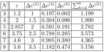
Apart from the two particle contribution (24), which is usually quite trivial and in this situation can even be evaluated analytically, we have carried out the multidi-mensional integrals in (22) by means of a Monte Carlo method. We use this method up to a precision which is higher than the last digit we quote. For convenience we report some explicit numbers in table 1.

N c ∆c(2) _∆c(4) _∆c(6) P6

k=2∆c(k)

3 1.2 1 0.197 0.002 1.199 4 2 1.5 0.394 0.096 1.990 5 2.857 2 0.591 0.191 2.782 6 3.75 2.5 0.788 0.285 3.573 7 4.¯6 3 0.985 0.380 4.365 8 5.6 3.5 1.182 0.474 5.156

Table 1: n-particle contributions to the c-theorem versus

SU(N)2/U(1)N−1 -WZNW coset model central charge.

The evaluation of (24)-(27) illustrates that the series (22) converges slower and slower for increasing values of

N, such that the highern-particle contributions become more and more important to achieve high accuracy. Our analysis suggests that it is not the functional dependence of the individual form factors which is responsible for this behaviour. Instead this effect is simply due to the fact that the symmetry factor, that is the sumP

µ1...µn, resulting from permutations of the particle species in-creases drastically for largerN.

Having confirmed the expected ultraviolet central charge, we now study the RG-flow by varyingr0in (23).

We expect to find that whenever we reach an energy scale at which an unstable particle can be formed, the model will flow to a different coset. This means following the flow with increasingr0 we will encounter a situation in

which certainσi,i+1are considered to be large and we

ob-serve the decoupling into two freely interacting systems in the way described in (2). For instance for the situ-ation σ12 > σ23 > σ34 > . . . we observe the following

decoupling along the flow with increasingr0:

SU(N)2/U(1)N−1

↓

SU(N−1)2/U(1)N−2⊗SU(2)2/U(1)

↓

SU(N−2)2/U(1)N−3⊗(SU(2)2/U(1))2

↓

.. .

↓

(SU(2)2/U(1))N−1

We can understand this type of behaviour in a semi-analytical way. The precise difference between the central charges related to (2) is

cSU(i+1)2/U(1)i⊗SU(N−i)2/U(1)N−i−1 = (28)

cSU(N)2/U(1)N−1−

2i(N+ 5)(N−i−1) (N+ 2)(i+ 3)(N −i+ 2).

Noting with (21) that we loose at each step all the con-tributionsFΘ|µiµi+1...

n (θ) to ∆c, we may collect the val-ues (24)-(26), which we have determined numerically and find

lim σi,i+1→∞

∆c(σ_i,i+1, . . .) = (29)

Similarly as for the deep UV-region we find a relatively good agreement between (28) and (29) for small values of N. The difference for larger values is once again due to the convergence behaviour of the series in (22).

For r0 = 0 qualitatively a similar kind of behaviour

was previously observed, for the two particle contribution only, in the context of the roaming Sinh-Gordon model [12]. Nonetheless, there is a slight difference between the two situations. Instead of a decoupling into different cosets in these type of models the entire S-matrix takes on the value−1, when the resonance parameter goes to infinity. The resulting effect, i.e. a depletion of ∆c, is the same. However, we do not comply with the interpre-tation put forward in [12], namely that such a behaviour should constitute a “violation of the c-theorem”. The observed effect is precisely what one expects from the physical point of view and the c-theorem.

We present our full numerical results in figure 1, which confirm the outlined flow for various values of N.

Figure 1: RG flow for the Virasoro central charge.

We observe that thec-function remains constant, at a value corresponding to the new coset, in some finite inter-val ofr0. In particular, we observe the non-equivalence of

the flows when the relative order of magnitude amongst the different resonance parameters is changed. ForN= 5 we confirm (we omit here theU(1)-factors and report the corresponding central charges as superscripts on the last factor)

σ12> σ23 SU(5)

20 7

2 σ23> σ12

ւ ց

SU(4)2⊗SU(2)

5 2

2 SU(3)2⊗SU(3)

12 5

2

ց ւ

SU(3)2⊗SU(2)2⊗SU(2)

11 5

2

↓

SU(2)2⊗SU(2)2⊗SU(2)2⊗SU(2)22

The precise difference in the central charges is ex-plained with (29), since the contribution 0.0924Ii,i−1only

occurs fori= 1.

To establish more clearly that the plateaus admit in-deed an interpretation as fixed points and extract the def-inite values of the corresponding Virasoro central charge we can also, following [11], determine a β type func-tion fromc(r). The β-function should obey the Callan-Symanzik equation [13]

rd

drg=β(g). (30)

The “coupling constant”g:=cuv−c(r) is normalized

in such a way that it vanishes at the ultraviolet fixed point. Whenever we findβ(˜g) = 0, we can identify ˜c =

cuv−g˜as the Virasoro central charge of the corresponding

conformal field theory. Hence, taking the data obtained from (23), we computeβ as a function of gby means of (30). Our results for various values of N are depicted in figure 2, which allow a definite identification of the fixed points corresponding to the coset models expected from the decoupling (2).

Figure 2: Theβ-function.

ForSU(4)2 we clearly identify from figure 2 the four

fixed points ˜g = 0,0.3,0.5,2 with high accuracy. The five fixed points ˜g = 0,0.357,0.657,0.857,2.857, which we expect to find forSU(5)2 are all slightly shifted due

to the absence of the higher order contributions.

V. OPERATOR CONTENT OFSU(N)2/U(1)N

−1

We now want to identify the operator content of our theory by carrying out the ultraviolet limit and match-ing the conformal dimension of each operator with the one in theSU(N)2/U(1)N−1-WZNW-coset model. For

this purpose we have to determine first of all the entire operator content of the conformal field theory.

According to [14] the conformal dimensions of the parafermionic vertex operators are given by

∆(Λ, λ) =(Λ·(Λ + 2ρ)) (4 + 2N) −

(λ·λ)

Here Λ is a highest dominant weight of level smaller or equal to 2 and ρ = 1/2P

α>0α is the Weyl vector, i.e.

half the sum of all positive roots. The λ’s are the cor-responding lower weights, which may be constructed in the usual fashion (see e.g. [15]): Consider a complete weight string λ+nα, . . . , λ, . . . , λ−mα, that is all the weights obtained by successive additions (subtractions) of a root α from the weight λ, such that λ+ (n+ 1)α

(λ−(m+ 1)α) is not a weight anymore. It is then a well known fact that the difference between the two integers

m, nism−n=λ·αfor simply laced Lie algebras. This means starting with the highest weight Λ, we can work our way downwards by deciding after each subtraction of a simple rootαi whether the new vector, say χ, is a weight or not from the criterion mi = ni+χ·αi > 0. With the procedure just outlined we obtain all possible weights of the theory. Nonetheless, it may happen that a weight corresponds to more than one linear independent weight vector, such that the weight space may be more than one dimensional. The dimension of each weight vec-tornΛ

λ is computed by means of

nΛλ = P

α>0 P∞

l=12nλ+lα((λ+lα)·α)

((Λ +λ+ 2ρ)·(Λ−λ)) . (32)

For consistency it is useful to compare the sum of all these multiplicities with the dimension of the highest weight representation computed directly from the Weyl dimen-sionality formula (see e.g. [15])

X

λ

nΛ

λ = dim Λ = Y

α>0

((Λ +ρ)·α)

(ρ·α) . (33)

To compute all the conformal dimensions ∆(Λ, λ) accord-ing to (31) in general is a formidable task and therefore we concentrate on a few distinct ones for genericN and only compute the entire content forN = 4.

Noting that λi· λj =Kij−1, withK being the Cartan matrix, we can obtain relative concrete formulae from (31). For instance

∆(λi, λi) =

4PN_l=1−1K_il−1−N K_ii−1

8 + 2N . (34)

Similarly we may compute ∆(λi+λj, λi+λj), etc. in terms of components of the inverse Cartan matrix. Even more explicit formulae are obtainable when we express the simple rootsαiand fundamental weightsλiofSU(N) in terms of a concrete basis. For instance we may choose an orthonormal basis {εi} in RN (see e.g. [16]), i.e. εi·

εj=δij

αi=εi−εi+1, λi= i X

j=1

εj−

i N

N X

j=1

εj, i= 1, . . . N−1.

Noting further that the set of positive roots is given by

{εi−εj: 1≤i < j≤N}, we can evaluate (31), (32) and (33) explicitly. This way we obtain for instance

∆(λi, λi) =

i(N−i)

8 + 4N and ∆(2λi,2λi) = 0. (35)

Of special physical interest is the dimension of the per-turbing operator. As was already argued in [3], it cor-responds to ∆(ψ,0), with ψbeing the highest root, and moreover it is unique. Noting that for SU(N) we have

ψ=λ1+λN−1, we confirm once more

∆(ψ=λ1+λN−1,0) =

N

N+ 2 . (36)

Other dimensions may be computed similarly.

A. TheSU(4)/U(1)3 _example

ForSU(4)/U(1)3 _{we present the result of the}

compu-tation of the entire operator content in table 2. In case the multiplicity of a weight vector is bigger than one, we indicate this by a superscript on the conformal dimen-sion.

λ\Λ λ1 λ2 2λ1 2λ2 λ1+λ2 λ1+λ3

dim Λ 4 6 10 20 20 15 Λ 1/8 1/6 0 0 1/8 1/6 Λ−α1 1/8 1/2 1/8 1/6

Λ−α2 1/6 1/2 1/8

Λ−α3 1/6

Λ−α1−α2 1/8 1/6 1/2 1/2 5/82 1/6

Λ−α2−α3 1/6 1/2 1/8 1/6

Λ−α1−α3 1/6

Λ−2α1 0

Λ−2α2 0

Λ−2α1−2α2 0 0

Λ−2α2−2α3 0

Λ−2α1−α2 1/2 1/8

Λ−α1−2α2 1/2 1/8

Λ−2α2−α3 1/2

Λ−α1−α2−α3 1/8 1/6 1/2 1/2 5/82 2/33

Λ−2α1−α2−α3 1/2 1/8 1/6

Λ−α1−2α2−α3 1/6 12 5/82 1/6

Λ−α1−α2−2α3 1/6

Λ−2α1−2α2−α3 1/2 1/2 5/82 1/6

Λ−α1−2α2−2α3 1/2 1/8 1/6

Λ−2α1−2α2 1/8

Λ−2α1−2α2−2α3 0 0 1/8 1/6

Λ−α1−3α2−2α3 1/2

Λ−α1−3α2−α3 1/2

Λ−2α1−3α2−α3 1/2 1/8

Λ−2α1−3α2−2α3 1/2 1/8

Λ−2α1−4α2−2α3 0

Table 2: Conformal dimensions for O∆(Λ,λ) in the

SU(4)2/U(1)3 -WZNW coset model.

The remaining dominant weights of level smaller or equal to 2, namely Λ =λ3,2λ3, λ2+λ3, including their

exchange 1↔3, which corresponds to theZ2-symmetry

of theSU(4)-Dynkin diagram.

Summing up all the fields corresponding to different lower weights, i.e. not counting the multiplicities, we have the following operator content

O2/3,O1,14× O0,8× O5/8,18× O1/6,24× O1/2,32× O1/8,

that is 98 fields.

VI. OPERATOR CONTENT OF HSG

We will now turn to the massive model and evaluate the flow of the conformal dimension [3]

∆O(r0) =−

1 2hO(0)i

∞

Z

r0

dr r hΘ(r)O(0)i . (37)

Here O is a local operator which in the conformal limit corresponds to a primary field in the sense of [17]. In particular forr0= 0, the expression (37) constitutes the

delta sum rule [18], which expresses the difference be-tween the ultraviolet and infrared conformal dimension of the operatorO.

We start by investigating the operator which in the case when all particles in (5) are of the same type cor-responds to the disorder operator µin the Ising model. Using the fact that we should always be able to reduce to that situation, we consider the solution corresponding to τi = ¯τi =νi =ςi = 0 for all i. Then the ∆-sum rule (37) yields for the individualn-particle contributions

∆µ(2)= (N−1)·0.0625 (38) ∆µ(4)_{= (2−N)·0.0263 (39)}

∆µ(6)= (N−2)·0.0017 + (3−N)·0.0113 (40)

6 X

k=2

∆µ(k)= 0.0266 +N∗0.0206. (41)

We assume that this solution has the conformal dimen-sion ∆(λ1, λ1) in the ultraviolet limit. For comparison we

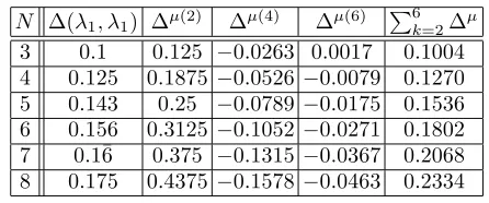
report a few explicit numbers in table 3.

N ∆(λ1, λ1) ∆µ(2) ∆µ(4) ∆µ(6) P6k=2∆µ

3 0.1 0.125 −0.0263 0.0017 0.1004 4 0.125 0.1875 −0.0526 −0.0079 0.1270 5 0.143 0.25 −0.0789 −0.0175 0.1536 6 0.156 0.3125 −0.1052 −0.0271 0.1802 7 0.1¯6 0.375 −0.1315 −0.0367 0.2068 8 0.175 0.4375 −0.1578 −0.0463 0.2334

Table 3: n-particle contributions to the ∆-theorem versus conformal dimensions in theSU(N)2/U(1)N

−₁

-WZNW coset model.

As we already observed for the c-theorem, the series converges slower for larger values of N. The reason for

this behaviour is the same, namely the increasing sym-metry factor. Note also that the next contribution is negative.

Following now the RG-flow for the conformal dimen-sion (37) by varyingr0, we assume that the ∆(λ1, λ1

)-field flows to the ∆(λ1, λ1)-field in the corresponding new

cosets. Similar as for the Virasoro central charge we may compare the exact expression

∆(λ1, λ1)SU(i+1)2/U(1)i⊗SU(N−i)2/U(1)N−i−1 = (42)

∆(λ1, λ1)SU(N)2/U(1)N−1+

i(N+ 5)(N−i−1) 4(N+ 2)(i+ 3)(N−i+ 2).

with the numerical results. The contributions (38)-(40) yield

lim σi,i+1→∞

∆µ(σi,i+1, . . .) = (43)

∆µ(σ_i,i+1= 0, . . .) + 0.0359I_i,i+1+ 0.0113Ii,i−1.

Once again we find good agreement between the two com-putations for small values ofN. Our complete numerical results are presented in figure 3, which confirm the out-lined flow for various values of N.

Figure 3: RG flow for the conformal dimension ofµ.

Notice by comparing the figures 3 and 1, that, as we expect, the transition from one value for ∆ to the one in the decoupled system occurs at the same energy scalet0

at which the value of the Virasoro central charge flows to the new one.

In analogy to (30) we may now define a function “β′_”

and demand that it obeys the Callan-Symanzik equation

r d drg

′_=β′_(g′_{). (44)}

The “coupling constant” related to β′ _{is normalized}

in such a way that it vanishes at the ultraviolet fixed point, i.e. g′ _{:= ∆(r)−∆}

uv, such that whenever we

find β′_(˜g′_{) = 0, we can identify ˆ∆ = ˜g}′ _−∆

uv as the

conformal dimension of the operator under consideration of the corresponding conformal field theory. From our analysis of (37) we may determineβ′ _{as a function ofg}′

Figure 4: Theβ′

-function .

Once again, forSU(4)2 the accuracy is very high and

we clearly read off from figure 4 the expected fixed points ˜

g′ _{= −0.125,0,0.0375,0.0625. The SU(5)}

2-fixed points

˜

g′ _{= −0.1429,0,0.0446,0.0821,0.1071, are once again}

slightly shifted.

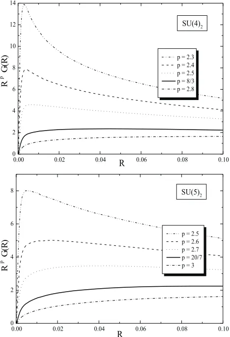
Figure 5: Rescaled correlation function G(R)=hΘ(R)Θ(0)i as a function ofR=rm.

Unfortunately, whenever the correlation function be-tween O and Θ is vanishing, or when we consider an

operator which does not flow to a primary field, we can not employ the delta sum rule (37). Alternatively, we may exploit the well known relation

lim

r→0hO(r)O(0)i ∼r

−4∆O

. (45)

near the critical point in order to determine the confor-mal dimension. To achieve consistency with the proposed physical picture we want to identify in particular the con-formal dimension of the perturbing operator. Recalling that the trace of the energy momentum tensor is propor-tional to the perturbing field we analysehΘ(R)Θ(0)ifor this purpose.

According to (45), we deduce from figure 5 ∆ = 2/3,5/7 for N = 4,5, respectively, which coincides with the expected values.

VII. CONCLUSIONS

One of the main deductions from our analysis is that the scattering matrix proposed in [6] may certainly be associated to the perturbed gauged WZNW-coset. This is based on the fact that we reproduce all the predicted features of this picture, namely the expected ultraviolet Virasoro central charge, various conformal dimensions of local operators and the characteristics of the unstable particle spectrum.

Our construction of general solutions to the form factor consistency equations certainly constitutes a further im-portant step towards a generic group theoretical under-standing of the n-particle form factor expressions. The next natural step is to extend the investigation towards higher level algebras [20].

Concerning the computation of correlation functions, our results also indicate that the “folkloristic belief” of the fast convergence of the series expansion of (22) has to be challenged. In fact, for large values of N, this is not true anymore. It would be highly desirable to have more concrete quantitative criteria at hand.

Despite the fact of having identified some part of the operator content, it remains a challenge to perform a def-inite one-to-one identification between the solutions to the form factor consistency equations and the local oper-ators. It is clear that we require new additional technical tools to do this, since the ∆-sum rule (37) may not be applied in all situations and (45) does not allow a clear cut deduction of ∆.

with the help of form factors only adds more terms to eachn-particle contribution, but is technically not more involved. The price we pay in this setting is, however, the slow convergence of (22).

We conjecture that the “cutting rule” which describes the renormalization group flow also holds for other groups. This is supported by the general structure of the HSG-scattering matrix.

Acknowledgments: A.F. is grateful to the Deutsche Forschungsgemeinschaft (Sfb288) for financial support. O.A.C. thanks CICYT (AEN99-0589), DGICYT (PB96-0960) and the Freie Universit¨at Berlin for partial finan-cial support and is also very grateful to the Institut f¨ur theoretische Physik of the Freie Universit¨at for hospital-ity. We would like to thank J.L. Miramontes for useful comments.

[1] O.A. Castro-Alvaredo, A. Fring and C. Korff, Phys. Lett.

B484(2000) 167.

[2] O.A. Castro-Alvaredo and A. Fring,Identifying the Oper-ator Content, the Homogeneous Sine-Gordon models hep-th/0008044.

[3] O.A. Castro-Alvaredo and A. Fring, Renormalization group flow with unstable particleshep-th/0008208. [4] C.R. Fern´andez-Pousa, M.V. Gallas, T.J. Hollowood and

J.L. Miramontes, Nucl. Phys. B484 (1997) 609; Q-H. Park,Phys. Lett.B328(1994) 329; T.J. Hollowood, J.L. Miramontes and Q-H. Park, Nucl. Phys. B445 (1995) 451.

[5] P. Goddard, A. Kent and D.Olive, Phys. Lett. B152

(1985) 88.

[6] J.L. Miramontes and C.R. Fern´andez-Pousa,Phys. Lett.

B472(2000) 392.

[7] R.J. Eden, P.V. Landshoff, D.I. Olive and J.C. Polk-inghorne, The analytic S-Matrix (CUP, Cambridge, 1966).

[8] P. Weisz,Phys. Lett.B67,179 (1977); M. Karowski and P. Weisz, Nucl. Phys.B139(1978) 445.

[9] F.A. Smirnov, “Form factors in Completely Integrable Models of Quantum Field Theory”, Adv. Series in Math. Phys.14(World Scientific, Singapore, 1992).

[10] M. Gell-Mann and F.E. Low,Phys. Rev.95(1954) 1300, E.C.G. St¨uckelberg and A. Peterman,Helv. Phys. Acta

26(1953) 499.

[11] A.B. Zamolodchikov,JETP Lett.43(1986) 730. [12] C. Ahn, G. Delfino and G. Mussardo, Phys. Lett.B317

(1993) 573.

[13] C.G. Callan, Phys. Rev.D2(1970) 1541; K. Symanzik,

Comm. Math. Phys.18(1970) 227.

[14] D. Gepner,Nucl. Phys.B290[FS20] (1987) 10.

[15] W. Fulton and J. Harris, Representation Theory

(Springer, Berlin, 1999).

[16] N. Bourbaki,Groupes et alg`ebres de Lie, Chapitres 4,5,6

(Masson, Paris, 1981).

[17] A.A. Belavin, A.M. Polyakov and A.B. Zamolodchikov,

Nucl. Phys.B241 (1984)333.

[18] G. Delfino, P. Simonetti and J.L. Cardy, Phys. Lett.

B387(1996) 327.

[19] O.A. Castro-Alvaredo, A. Fring, C. Korff and J.L. Mira-montes,Nucl. Phys.B573(2000) 535.