Adaptive Feature Ranking for Unsupervised Transfer Learning

City, University of London Institutional Repository

Citation

:

Tran, S. N. and Garcez, A. Adaptive Feature Ranking for Unsupervised Transfer

Learning. .

This is the draft version of the paper.

This version of the publication may differ from the final published

version.

Permanent repository link:

http://openaccess.city.ac.uk/19149/

Link to published version

:

Copyright and reuse:

City Research Online aims to make research

outputs of City, University of London available to a wider audience.

Copyright and Moral Rights remain with the author(s) and/or copyright

holders. URLs from City Research Online may be freely distributed and

linked to.

Adaptive Feature Ranking for Unsupervised Transfer

Learning

Son N. Tran

Department of Computer Science City University London London, UK, EC1V 0HB Son.Tran.1@city.ac.uk

Artur d’Avila Garcez

Department of Computer Science City University London London, UK, EC1V 0HB aag@soi.city.ac.uk

Abstract

Transfer Learning is concerned with the application of knowledge gained from solving a problem to a different but related problem domain. In this paper, we propose a method and efficient algorithm for ranking and selecting representa-tions from a Restricted Boltzmann Machine trained on a source domain to be transferred onto a target domain. Experiments carried out using the MNIST, IC-DAR and TiCC image datasets show that the proposed adaptive feature ranking and transfer learning method offers statistically significant improvements on the training of RBMs. Our method is general in that the knowledge chosen by the ranking function does not depend on its relation to any specific target domain, and it works with unsupervised learning and knowledge-based transfer.

Keywords: Feature Selection, Transfer Learning, Restricted Boltzmann Machines

1

Introduction

Transfer Learning is concerned with the application of knowledge gained from solving a problem to a different but related problem domain. A number of researchers in Machine Learning have argued that the provision of supplementary knowledge should help improve learning performance [15, 2, 12, 1, 11, 14, 9, 3]. In Transfer Learning [10, 1, 11, 14], knowledge from a source domain can be used to improve performance in a target domain by assuming that related domains have some knowledge in common. In connectionist transfer learning, many approaches transfer the knowledge selected specifically based on the target, and (in some cases) with the provision of labels in the source domain [8, 16]. In constrast, we are interested in selecting the representations that can be transferred in general to the target without the provision of labels in the source domain, which is similar to self-taught learning [11, 6]. In addition, we propose to study how much knowledge should be transferred to the target domain, which has not been studied yet in self-taught mode.

This paper introduces a method and efficient algorithm for ranking and selecting representation knowledge from a Restricted Boltzmann Machine (RBM) [13, 4] trained on a source domain to be transferred onto a target domain. A ranking function is defined that is shown to minimize infor-mation loss in the source RBM. High-ranking features are then transferred onto a target RBM by setting some of the network’s parameters. The target RBM is then trained to adapt a set of additional parameters on a target dataset, while keeping the parameters set by transfer learning fixed.

Experiments carried out using the MNIST, ICDAR and TiCC image datasets show that the proposed adaptive feature ranking and transfer learning method offers statistically significant improvements on the training of RBMs in three out of four cases tested, where the MNIST dataset is used as source and either the ICDAR or TiCC dataset is used as target. As expected, our method improves on the predictive accuracy of the standard self-taught learning method for unsupervised transfer learning [11].

Our method is general in that the knowledge chosen by the ranking function does not depend on its relation to any specific target domain. In transfer learning, it is normal for the choice of the knowledge to be transferred from the source domain to rely on the nature of the target domain. For example, in [7], knowledge such as data samples in the source domain are transformed to a target domain to enrich supervised learning. In our approach, the transfer learning is unsupervised, as done in [11]. We are concerned with inductive transfer learning in that representation learned from a domain can be useful in analogous domains. For example, in [1] a common orthonormal matrix is learned to construct linear features among multiple tasks. Self-taught learning [11], on the other hand, applies sparse coding to transfer the representations learned from source data onto the target domain. Like self-taught, we are interested in unsupervised transfer learning using cross-domain features. The system has been implemented in MATLAB; all learning parameters and data folds are available upon request.

The outline of the paper is as follows. In Section 2, we define feature selection by ranking in which high scoring features are associated with significant part of the network. In Section 3, we introduce the adaptive feature learning method and algorithm to combine selective features in source domain with features in target domain. In Section 4, we present and discuss the experimental results. Section 5 concludes and discusses directions for future work.

2

Feature Selection by Ranking

In this section, we present a method for selecting representations from an RBM by ranking their features. We define a ranking function and show that it can capture the most significant information in the RBM, according to a measure of information loss.

In a trained RBM, we definecjto be a score for each unitjin the hidden layer. The score represents the weight-strength of a sub-networkNj(hj ∼V) consisting of all the connections from unitjto the visible layer. A scorecjis a positive real number that can be seen as capturing the uncertainty in the sub-network. We expect to be able to replace all the weights of a network by appropriatecj or−cjwith minimum information loss. We define the information loss as:

Iloss=

X

j

kwj−cjsjk2 ₍₁₎

wherewj is a vector of connection weights from unitj in the hidden layer to all the units in the visible layer,sjis a vector of the same sizevisNaswj, andsj ∈[−1 1]visN_.

Since equation (1) is a quadratic function, the value ofcj that minimizes information loss can be found by setting the derivatives to zero, as follows:

X

i

2(wij−cjsij)sij = 0with allj

X

i

wijsij−cj

X

i

s2_ij = 0with allj

cj=

P

iwijsij

P

is

2

ij

(2)

Sincesij = [−1 1]and from equation (1), we can see that:

kwij−cjsijk2=kabs(wij)−cj

sij

sign(wij)

k2_{≥ kabs(w}

ij)−cjk2 (3) holds if and only ifsij =sign(wij), which will also minimizeIloss.

Applying equation (3) to (2), we obtain:

cj=

P

iabs(wij)

We may notice that using cj instead of weights would result in a compression of the network; however, in this paper we focus on the scores only for selecting features to use for transfer learning. In what follows, we give a practical example which shows that low-score features are semantically less meaningful than high-scoring ones.

Example 2.1 We have trained an RBM with 10 hidden nodes to model the XOR function from its truth-table such thatz=xXORy. Thetrue, f alselogical values are represented by integers1,0, respectively. After training the network, a score for each sub-network can be obtained. The score allows us to replace each real-value weight by its sign, and interpret those signs logically where a negative sign (−) represents logical negation (¬), as exemplified in Table 1.

Network Sub-network Symbolic representation

2.970 :h2∼ {+x,−y,+z}

can be interpreted as

z=x∧ ¬y

with score2.970

Table 1: RBM trained on XOR function and one of its sub-networks with score value and logical interpretation

Table 2 shows all the sub-networks with associated scores. As one may recognize, each sub-network represents a logical rule learned from the RBM. However, not all of the rules are correct w.r.t. the XOR function. In particular, the sub-network scoring0.158encodes a rule¬z =¬x∧y, which is inconsistent withz=xXORy. By ranking the sub-networks according to their scores, this can be identified: high-scoring sub-networks are consistent with the data, and low-scoring ones are not. We have repeated the training several times with different numbers of hidden units, obtaining similar intuitive results.

Score Sub-network Logical Representation 1.340 h1∼ {+x,−y,+z} z=x∧ ¬y

2.970 h2∼ {+x,−y,+z} z=x∧ ¬y

6.165 h3∼ {−x,+y,+z} z=¬x∧y

0.158 h4∼ {−x, y,−z} ¬z=¬x∧y

2.481 h5∼ {+x,−y,+z} z=x∧ ¬y

1.677 h6∼ {−x,+y,+z} z=¬x∧y

2.544 h7∼ {+x,−y,+z} z=x∧ ¬y

7.355 h8∼ {+x,+y,−z} ¬z=x∧y

6.540 h9∼ {−x,−y,−z} ¬z=¬x∧ ¬y

4.868 h10∼ {−x,−y,−z ¬z=¬x∧ ¬y

Table 2: Sub-networks and scores from RBM with 10 hidden units trained on XOR truth-table

In what follows, we will study the effect of pruning low-scoring sub-networks from an RBM trained on complex image domain data. So far, we have seen that our scoring can be useful at identifying relevant representations. In particular, if the score of a sub-network is small in relation to the average score of the network, they seem more likely to represent noise.

3

Adaptive Feature Learning

improving the predictive accuracy of another RBM trained on a target domain. From a transfer learning perspective, we intend to produce a general transfer learning algorithm, ranking knowledge from a source domain to guide the learning on a target domain, using RBMs as transfer medium. In particular, we propose a transfer learning model as shown in Figure 1. Knowledge learned from a source domain is selected by the ranking function for transferring onto a target domain, as explained in what follows. The selection of features in the source domain is general in that it is independent from the data from the target domain.

Figure 1: General adaptive feature transfer mechanism for unsupervised learning

In the target domain, an RBM is trained given a number of transferred parameters (W(t)_{): a fixed}

set of weights associated with high-ranking sub-networks from the source domain. The output of transferred hidden nodes in target domain is considered as self-taught features [11]. The connections between the visible layer and the hidden units transferred onto the target RBM can be seen as a set of up-weights and down-weights. How much the down-weights affect the learning in the target RBM depends on an influence factorθ; in this paperθ∈[0 1]. Ifθ= 0then the features are combined but the transferred knowledge will not influence learning in the target domain. In this case, the result is a combination of self-taught features and target RBM features. Otherwise, ifθ= 1then the transferred knowledge will influence learning in the target domain. We refer to this case as adaptive feature learning, because the knowledge transferred from the source domain is used to guide the learning of new features in the target domain. The outputs of additional hidden nodes (associated with parameterU) in target RBM are called adaptive features.

As usual, we train the target RBM to maximize the log-likelihood:

L(U|D;W(t)) (5) using Contrastive Divergence [4].

Algorithm 1Adaptive feature learning

Require: A trained RBMN

1: Select a number of sub-networksN(t)_{∈N with the highest scores}

2: Encode parametersW(t)_fromN(t)_{into a new RBM}

3: Add hidden units (U) to the RBM

4: loop

5: % until convergence

6: V+⇐X

7: H+←p(H|V+); Hˆ+

smp

← p(H|V+); 8: V−←p(V|Hˆ+); Vˆ−

smp

← p(V|Hˆ+) 9: H−←p(H|Vˆ−)

10: Y =U+η(hV+TH (t)

+ −Vˆ

T

−H−(t)i) 11: end loop

4

Experimental Results

we show that knowledge from one image domain can be used to improve predictive accuracy in another image domain.

4.1 Feature Selection

We have trained an RBM with 500 hidden nodes on 20,000 samples from the MNIST dataset in order to visualized the filter bases of the50highest scoring sub-networks and the50lowest scoring sub-networks (each takes10%of the network’s capacity). Figure 2 shows the result of using a standard RBM, and Figure 3 shows the result of using a sparse RBM [6]. As can be seen, in Figure 2, high scores are mostly associated with more concrete visualizations of the expected MNIST patterns, while low scores are mostly associated with fading or noisy patterns. In Figure 3, high-scores are associated with sparse representations, while low-scores produce less meaningful representations according to the way in which the RBM was trained. In sparse RBM we use PCA to reduce the dimensionality of the images to69and train the network with Gaussian visible units.

(a) Filter bases with high scores (b) Filter bases with low scores

Figure 2: Features learned from RBM on MNIST dataset

(a) Filter bases with high scores (b) Filter bases with low scores

Figure 3: Learned features from sparse RBM on MNIST dataset

We also examined visually theimpactof the scores on an RBM with 500 hidden units trained on the MNIST dataset’s 10,000 examples. Sub-networks with the highest scores were gradually removed, and the pruned RBM was compared on the reconstruction of images with that of the original RBM, as illustrated in Figure 4. In Figure 5 we shows the reconstruction of test images from RBMs in which low-scored features were gradually removed.

Figure 4: Reconstructed test images from RBM in which high-scored features have been pruned. From left to right, number of hidden unit remain: 500 (full), 400 ,300, 200 and 100

Figure 5: Reconstructed test images from RBM in which low-scored features have been pruned. From left to right, number of hidden unit remain: 500 (full), 400 ,300, 200 and 100

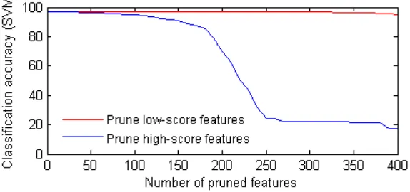
units have produced a slight increase in accuracy. Then, the results indicate that it is possible to remove nodes and maintain performance almost unchanged (until relevant units start to be removed, at which point accuracy deteriorates, when more than half of the number of units is removed). In case of pruning high-scored features, the accuracy decreases significantly when more than10%of hidden units are removed.

Figure 6: Classification accuracy of a pruned RBM, starting with 500 hidden units, on 10,000 MNIST test samples. The red line presents the pruning performance of low-scored features and the blue line presents the pruning performance of high-score features

4.2 Unsupervised Transfer Learning

In order to evaluate transfer learning in the context of images, we have transferred sub-networks from an RBM trained on the MNIST1_{dataset to RBMs trained on the ICDAR}2_{and TiCC datasets}3_.

Below, we use MNIST30kand MNIST05Kto denote datasets with 30,000 and 5,000 samples from the MNIST data collection. For the TiCC collection, we denote TiCCdand TiCCaas the datasets of digits and letters, respectively. TiCCcand TiCCware character samples from two different groups of writers. TiCCw Aand TiCCw Bare from the same group but the latter has a much smaller training set. Each column in Table 3 indicates a transfer experiment, e.g. MNIST30k : ICDARd uses the

1

http://yann.lecun.com/exdb/mnist/

2

http://algoval.essex.ac.uk:8080/icdar2005/index.jsp?page=ocr.html

3

MNIST dataset as source domain and ICDAR as target domain. The percentages show the predictive accuracy on the target domain, as detailed in the sequel.

MNIST30k: ICDARd MNIST30k: TiCCw A MNIST05k: TiCCa MNIST05k: TiCCd

SVM 39.04 73.44 59.16 60.34

PCA STL 39.38 68.36 57.90 56.29

SC STL 46.23 70.06 55.82 57.78

RBM STL 30.47±0.054 72.88±0.098 58.13±0.205 62.08±0.321

RBM 37.63±0.505 75.20±0.745 62.85±0.079 63.42±0.090

ASTL (α= 0) 36.66±0.495 76.49±0.361 63.21±0.134 65.04±0.330 ASTL (α= 1) 40.43±0.328 77.56±0.564 63.00±0.160 65.82±0.262

Table 3: Transfer learning experimental results: each column indicates a transfer experiment, e.g. MNIST30k: ICDARduses the MNIST dataset as source domain and ICDAR as target domain. The percentages show the predictive accuracy on the target domain. Results for SVMs are provided as a baseline. For the ”SVM” and ”RBM” lines, there is no transfer; for the other lines, transfer is carried out as described in Section??and Section??. The percentages show the average results with95% confidence interval

In Table 3, we have measured classification performance when using the knowledge from the source domain to guide the learning in the target domain. For each domain, the data is divided into training, validation and test sets. Each experiment is repeated 50 times and we use the validation set to se-lect the best model (number of transferred sub-networks, number of added units, learning rates and SVM hyper-parameters). The table reports the average results on the test sets. The results show that the proposed adaptive feature ranking and transfer learning method offers statistically significant improvements on the training of RBMs in three out of four cases tested, where the MNIST dataset is used as source and either the ICDAR or TiCC dataset is used as target. As expected, our method improves on the predictive accuracy of the standard self-taught learning method for unsupervised transfer learning. In order to compare with transferring low-scored features, we performed exper-iments follows what we have done with transferring high-scored features, except that in this case the features are ranked from low-scores to high-scores. We observed that the highest accuracies were achieved only when a large number of high-scored features are among those which have been transferred.

TiCCd: TiCCa TICCa: TiCCd TICCc: TICCw B

SVM 59.16 60.34 40.67

RBM STL 60.65±0.075 64.85±0.227 47.46±0.260 RBM 62.85±0.079 63.42±0.090 44.28±0.323 ASTL (α= 0) 62.41±0.166 66.10±0.137 51.07±0.684 ASTL (α= 1) 63.16±0.120 66.25±0.175 43.10±0.332

Table 4: Transfer learning experimental results for datasets in TiCC collection. The percentages show the average predictive accuracy on the target domain with95%confidence interval

We also carried out experiments on the TiCC collection transferring from characters to digits, digits to characters, and from group of writers to group of other writers. The results in Table 4 show that in two out of three experiments adaptive learning and combining features did not gain advantages over combination of selective features from source domain and features from target domain. It may suggest that using selective combination of features would be better and more efficient in a case that the source and target domains are considerably similar(i.e TiCCc:TICCw B)

To compare our transfer learning approach with self-taught learning [11], we train an RBM in the source domain and use it to extract common features in the target domain for classification. In the experiments where the domains have a close relation such as the same type of data (digits in MNIST05k:TiCCd) or in the same collections (TiCCd:TiCCa,TiCCd:TiCCd,TiCCc:TiCCwB), sefl-taught learning works very well especially when the training dataset in the target domain is small (TiCCc:TiCCwB). We also use sparse-coder [5] provided by Lee4 for self-taught learning as in [11], except that instead of using PCA for preprocessing data we apply the model directly to the raw

4

(a) MNIST to ICDAR digits (b) MNIST to TiCC letters

(c) MNIST to TiCC digits (d) MNIST to TiCC writers

Figure 7: Performance of self-taught learning using RBM and sparse-coder regarding to number of bases/hidden units

pixels since that is what has been done with the RBM. Figure 7 shows the performance of self-taught learning on the datasets using RBMs and sparse-coder as feature learners.

(a) MNIST to ICDAR (b) MNIST to TiCC digits (c) MNIST to TiCC letters

(d) MNIST to TiCC writers (e) TiCC letters to TiCC digits (f) TiCC digits to TiCC letters

Figure 8: Performance of learning with guidance for different numbers of transferred knowledge rules and additional hidden units. The colour-bars map accuracy to the colour of the cells as shown so that the hotter the color, the higher the accuracy.

5

Conclusion and Future Work

We have presented a method and efficient algorithm for ranking and selecting representations from a Restricted Boltzmann Machine trained on a source domain to be transferred onto a target domain. The method is general in that the knowledge chosen by the ranking function does not depend on its relation to any specific target domain, and it works with unsupervised learning and knowledge-based transfer. Experiments carried out using the MNIST, ICDAR and TiCC image datasets show that the proposed adaptive feature ranking and transfer learning method offers statistically significant improvements on the training of RBMs.

In this paper we focus on selecting features from shallow network (RBM) for general transfer learn-ing. In future work we are interested in learning and transferring high-level features from deep networks selectively for a specific domain.

References

[1] Andreas Argyriou, Theodoros Evgeniou, and Massimiliano Pontil. Multi-task feature learning. InAdvances in Neural Information Processing Systems 19. MIT Press, 2007.

[2] Artur S. Avila Garcez and Gerson Zaverucha. The connectionist inductive learning and logic programming system. Applied Intelligence, 11(1):5977, July 1999.

[3] Jesse Davis and Pedro Domingos. Deep transfer via second-order markov logic. In Pro-ceedings of the 26th Annual International Conference on Machine Learning, ICML ’09, page 217224, New York, NY, USA, 2009. ACM.

[4] Geoffrey E. Hinton. Training products of experts by minimizing contrastive divergence.Neural Comput., 14(8):1771–1800, August 2002.

[5] Honglak Lee, Alexis Battle, Rajat Raina, and Andrew Y. Ng. Efficient sparse coding algo-rithms. In B. Sch¨olkopf, J. Platt, and T. Hoffman, editors,Advances in Neural Information Processing Systems 19, pages 801–808. MIT Press, Cambridge, MA, 2007.

[6] Honglak Lee, Chaitanya Ekanadham, and Andrew Y. Ng. Sparse deep belief net model for visual area v2. InAdvances in Neural Information Processing Systems. MIT Press, 2008.

[7] Joseph J. Lim, Ruslan Salakhutdinov, and Antonio Torralba. Transfer learning by borrowing examples for multiclass object detection. InNIPS, pages 118–126, 2011.

[8] Gr´egoire Mesnil, Yann Dauphin, Xavier Glorot, Salah Rifai, Yoshua Bengio, Ian J. Goodfel-low, Erick Lavoie, Xavier Muller, Guillaume Desjardins, David Warde-Farley, Pascal Vincent, Aaron C. Courville, and James Bergstra. Unsupervised and transfer learning challenge: a deep learning approach. InICML Unsupervised and Transfer Learning, pages 97–110, 2012.

[9] Lilyana Mihalkova, Tuyen Huynh, and Raymond J. Mooney. Mapping and revising markov logic networks for transfer learning. InProceedings of the 22nd national conference on Artifi-cial intelligence - Volume 1, AAAI’07, page 608614. AAAI Press, 2007.

[10] Sinno Jialin Pan and Qiang Yang. A survey on transfer learning.IEEE Transactions on Knowl-edge and Data Engineering, 22(10):1345–1359, October 2010.

[11] Rajat Raina, Alexis Battle, Honglak Lee, Benjamin Packer, and Andrew Y. Ng. Self-taught learning: transfer learning from unlabeled data. InProceedings of the 24th international con-ference on Machine learning, ICML ’07, page 759766, New York, NY, USA, 2007. ACM.

[12] Matthew Richardson and Pedro Domingos. Markov logic networks. Mach. Learn., 62(1-2):107136, February 2006.

[13] Paul Smolensky. Information processing in dynamical systems: Foundations of harmony the-ory. InIn Rumelhart, D. E. and McClelland, J. L., editors, Parallel Distributed Processing: Volume 1: Foundations, pages 194–281. MIT Press, Cambridge, 1986.

[14] Lisa Torrey, Jude W. Shavlik, Trevor Walker, and Richard Maclin. Transfer learning via advice taking. InAdvances in Machine Learning I, pages 147–170. Springer, 2010.