An adaptive stabilized finite element method for the generalized Stokes problem

An adaptive stabilized finite element method

for the generalized Stokes problem

Rodolfo Araya

Gabriel R. Barrenechea

and Abner Poza

Departamento de Ingenier´ıa Matem´atica Universidad de Concepci´on Casilla 160-C, Concepci´on, Chile

Abstract

In this work we present an adaptive strategy (based on an a posteriori error estima-tor) for a stabilized finite element method for the Stokes problem, with and without a reaction term. The hierarchical type estimator is based on the solution of local problems posed on appropriate finite dimensional spaces of bubble-like functions. An equivalence result between the norm of the finite element error and the estima-tor is given, where the dependence of the constants on the physics of the problem is explicited. Several numerical results confirming both the theoretical results and the good performance of the estimator are given.

Key words: Stokes equation, a posteriori error estimator, bubble function, stabilized finite element method, adapted mesh

1 Introduction

A posteriori error analysis and adaptive finite element methods for prob-lems in fluid dynamics has been a very active subject of research in the last decades. For instance, for the advective-diffusive model we can quote the works [22,17,5,6], among others. Now, for the Stokes problem, the works by Verf¨urth

Email addresses: [email protected] (Rodolfo Araya),

[email protected] (Gabriel R. Barrenechea),[email protected]

(Abner Poza).

[20,21] and Bank and Welfert [7], laid the basic foundation for the mathe-matical analysis of practical methods (see also [11] for error estimators in the nonconforming case). More recently, in [3,2] and [12], a posteriori error esti-mators rigorously bounding the discretization errors have been addressed. All previous references deal with stable (in the sense of the discrete inf-sup condi-tion [9]) discretizacondi-tions for the Stokes problem. In [18] and [4], an a posteriori error analysis of stabilized formulations for the Stokes problem was performed, but the analysis was restricted to the pure Stokes case (i.e., without a reaction term).

In this paper we introduce and analyze from theoretical and experimental points of view an adaptive scheme to efficiently solve the generalized Stokes problem. The scheme is based on the unusual stabilized finite element method introduced in [8], combined with an error estimator which is based on an idea from [2], building an auxiliary problem, whose solution is equivalent with the norm of the finite element error. Since this auxiliary problem is posed on an infinite dimensional setting, we build a hierarchical estimation for the solution of this problem, which turns out to be equivalent with the norm of its solution, and hence the resulting finite element approximation is equivalent to the original finite element error.

An outline of the paper is as follows. The model problem is stated in Section 2, and the bases of the discrete approximation are settled in Section 3. Next, in Section 4 we propose the auxiliary problem and prove that we can define a norm based on the solution of this auxiliary problem, which is equivalent to the norm of the error. This auxiliary problem is applied to the solution of the residual equation and hence we state, at the end of Section 4.1, a first equivalence result between the norm of the error and the solution of the auxiliary problem (with the residual as right-hand side). As we told before, the auxiliary problem is posed on an infinite dimensional space, and hence in Section 5 we define a finite dimensional approximation (based on a hierarchical idea) of its solution. Finally, in Section 6 we present several numerical results confirming the theoretical results and showing the good performance of our estimator, and in Section 7 we give some conclusions.

2 The model problem

Let Ω ⊆ R2 _{be a bounded open set with polygonal boundary Γ. We}

de-note by Hm_{(Ω) the usual Sobolev space of order m ≥ 0, with norm k· k} m,Ω and seminorm _{|· |}m,Ω, respectively (with the convention H0(Ω) = L2(Ω) and

Stokes problem reads: Find a velocity u and the pressure field p such that

(P)

            

σu₋ν∆u+_∇p = f in Ω,

div u = 0 in Ω,

u = 0 on Γ.

Let then H:=H1

0(Ω)2 and Q:=L20(Ω) :={q ∈ L2(Ω) : (q,1)Ω = 0}, where (_·,_·)D stands for the inner product in L2(D) (or inL2(D)2, L2(D)2×2, if

nec-essary) be the functional spaces to be used. The weak formulation of the problem (P) reads:Find (u, p)∈H_×Q such that

a(u,v) +b(v, p) +b(u, q) = (f,v)Ω ∀(v, q)∈H_×Q, (2.1)

where

a(u,v) := σ(u,v)Ω+ν(∇u,∇v)Ω, (2.2)

b(v, q) := ₋(q,divv)Ω. (2.3)

Furthermore, let c:Q×Q→R _{be the symmetric bilinear form defined by:}

c(p, q) := 1

ν (p, q)Ω.

Using bilinear forms a and c we define the following norms:

kv_ka := a(v,v)1/2 ∀v ∈H,

kqkc := c(q, q)1/2 ∀q∈Q ,

and the following norm on the product space H_×Q:

k(v, q)_k:=

(

kv_k2_a+_kq_k2_c

)1/2

∀(v, q)_∈H_×Q. (2.4)

The following result states the main properties of these bilinear forms.

Lemma 1 Let a andb be the bilinear forms given by (2.2) and (2.3), respec-tively. Then

|a(v,w)| ≤ kv_kakw_{ka ∀}v,w _∈H, (2.5)

|b(v, q)| ≤√2kv_kakqkc ∀(v, q)∈H ×Q , (2.6)

sup v_∈H

b(v, q)

kv_ka ≥

αb

s

ν

σ+ν kqkc ∀q ∈Q , (2.7)

PROOF. The proof follows from the norms definition and the well-known properties of these bilinear forms (see Theorem 4.1 in [15]). 2

Then, using the classical theory of Babuska-Brezzi (cf. [15]), we can state the following result.

Lemma 2 The weak problem (2.1) has a unique solution (u, p)∈H_×Q.

3 Notations and preliminary results

Let _{Th}h>0 be a regular family of triangulations of Ω and let us denote by

Eh the set of all sides of Th with the usual splitting Eh = EΩ ∪ EΓ, where EΩ stands for the sides lying on the interior of Ω. Also, for T ∈ Th, we denote by

N(T) the set of nodes ofT and by_E(T) the set of sides ofT. Also, forT _{∈ T}h

and F _{∈ E}h we define the following neighborhoods:

ωT :=

[

E(T)∩E(T′_)6=∅

T′ , ωeT :=

[

N(T)∩N(T′_)6=∅

T′,

ωF:=

[

F∈E(T′₎

T′ , ωeF :=

[

N(F)∩N(T′_)6=∅

T′.

Next, forT ∈ Th and F ∈ EΩ, let hT be the diameter of T,hF :=|F|, and let

us define the following mesh-dependent constants:

θT :=

    

ν−1/2_h

T , σ= 0,

σ−1/2 _min{h

T σ1/2ν−1/2,1} , σ >0.

θF :=

    

ν−1/2_h1/2

F , σ = 0,

ν−1/4_σ−1/4 _min{h

Fσ1/2ν−1/2,1}1/2 , σ > 0.

In the rest of the paper we will use the notation

ab _⇐⇒a _≤K b,

a_≃b _⇐⇒a b and ba,

where the positive constant K is independent of h, σ and ν.

Hh := {ϕ∈C(Ω)2 : ϕ|T ∈Pk(T)2, ∀T ∈ Th} ∩H01(Ω)2,

Qh := {ϕ∈C(Ω) : ϕ|T ∈Pl(T), ∀T ∈ Th} ∩L20(Ω).

Lemma 3 The following estimates hold for all vh ∈Hh and σ≥0:

k∇vhk0,T hT−1θT kvhka,T , (3.1)

k∆vhk0,T hT−2θT kvhka,T . (3.2)

PROOF. Ifσ = 0 the proof follows from the inverse inequality

k∇v_hk0,T h−_T1_kv_{hk0,T ∀}v_{h ∈}H_h, (3.3)

(see Lemma 1.138 in [14]) and the definition of θT. For σ > 0, from the

definition of _{k · k}a,T we see that

k∇vhk0,T ≤ν−1/2kvhka,T. (3.4)

On the other hand, using the inverse inequality (3.3) we obtain

k∇vhk0,T hT−1kvhk0,T h−T1σ−1/2kvhka,T. (3.5)

Then (3.1) arises using (3.4)-(3.5). For the second estimate, (3.3) and (3.1) lead to

k∆vhk0,T h−T1k∇vhk0,T h−T2θT kvhka,T,

and the result follows. 2

Let now Ih : H −→ Hh denote the Cl´ement interpolation operator (cf.

[10,15]). For all T _{∈ T}h and all F ∈ E(T) this operator satisfies

|v₋Ihv|m,T hTn−m|v|n,_eωT , (3.6)

kv₋Ihvk0,Fh n−1

2

F |v|n,_eωF , (3.7) for all v _∈ Hn_(Ω)2_{, and all 0 ≤ m ≤ 1, 1 ≤ n ≤ k+ 1. The following result} holds for the Cl´ement interpolation operator:

Lemma 4 For all T _{∈ T}h, F ∈ E(T), v ∈H1(Ω)2, there holds

kv₋Ihvk0,T θT kvka,_eωT, (3.8)

kv₋Ihvk0,FθFkvka,_eωF, (3.9)

PROOF. First and third estimates arise using (3.6)-(3.7), the previous lemma and the mesh regularity. In order to prove the second one, from [22], Lemma 3.1, we obtain

kv₋Ihvk0,F hT−1/2kv−Ihvk0,T +kv−Ihvk10/,T2|v−Ihv|11/,T2. (3.11)

Then, using (3.11) and (3.8) we arrive at

kv₋Ihvk0,FhT−1/2θT kvka,_eωT +ν

−1/4_θ1/2

T kvka,_eωT

"

h−_T1/2θT +ν−1/4θ1T/2

#

kv_ka,eωT .

Finally, since the mesh is regular

h−_T1/2θT +ν−1/4θT1/2=ν−1/4σ−1/4 min{hTν−1/2σ1/2,1}1/2×

"

1 + min{1, h−_T1ν1/2σ−1/2}1/2

#

θF,

and the second estimate follows. 2

Corollary 5 For all φ_∈H, the following estimates hold

X

T∈Th

θ−_T2kφ₋Ihφk20,Ta(φ,φ),

X

F∈ EΩ

θ−_F2kφ₋Ihφk20,Fa(φ,φ).

PROOF. First, from (3.8) and the mesh regularity we obtain

X

T∈Th

θ−_T2kφ₋Ihφk20,T

X

T∈Th

θ_T−2θ2_T kφ_k2_a,eω

T a(φ,φ).

Next, from (3.9) and the mesh regularity we obtain the second estimate. 2

4 The auxiliary problem

Let (e, E)_∈H _×Q, and let us define (φ, ψ)_∈H _×Qas the solution of the weak problem:

The well-posedeness of this problem arises from the fact that a and c are elliptic bilinear forms on H and Q, respectively.

Let||| · ||| :H_×Q→R_{be the mapping defined by}

(e, E)_{7−→ |||}(e, E)_|||:=

(

kφ_k2_a+_kψ_k2_c

)1/2

, (4.2)

where (φ, ψ) is the solution of (4.1).

Lemma 6 The mapping (4.2) defines a norm on H_×Q.

PROOF. Since_{k · k}a and k · kc are norms onH and Q, respectively, we only

have to prove that |||(e, E)|||= 0 implies (e, E) =0. If |||(e, E)||| = 0, then

a(e,v) +b(v, E) +b(e, q) = 0 _∀(v, q)_∈H _×Q . (4.3)

If we consider v =0 in (4.3), then e _∈ Ker(div ). Next, if q = 0 and v = e, then b(e, E) = 0 and hence a(e,e) = 0, which implies e = 0. Finally, since e=0, we have

(E,divv)Ω = 0 ∀v ∈H,

and, since div : H _−→ Q is a surjective operator, there exists v _∈ H, such that divv =E. HenceE = 0. 2

The next result shows the equivalence between ||| · ||| and (2.4).

Theorem 7 There exists a positive constant K2, independent of σ and ν,

such that

1

4|||(e, E)||| 2

≤ ke_k2_a+_kE_k2

c ≤K2

_σ+ν

ν

2

|||(e, E)_|||2,

for all (e, E)∈H_×Q.

PROOF. Upper bound: Using (2.7), q = 0 in (4.1), Cauchy-Schwarz’s in-equality and (2.5), we have

αb

s

ν

σ+ν kEkc ≤ vsup_∈H

|b(v, E)| kv_ka

= sup v∈H

|a(φ,v)₋a(e,v)_|

and then

kEkc ≤α−b1

s

σ+ν ν

(

kφ_ka+keka

)

. (4.4)

Now, considering q = −E, v = e in (4.1), using (2.5), Cauchy-Schwarz’s inequality and (4.4), we obtain

ke_k2_a=a(e,e)

=a(φ,e)₋c(ψ, E)

≤ kφ_kakeka+kψkckEkc

≤

(

kφ_ka+α−_b1

s

σ+ν ν kψkc

)

ke_ka+α_b−1

s

σ+ν

ν kψkckφka

≤1₂

(

kφ_ka+α−b1

s

σ+ν ν kψkc

)2 +1

2kek 2

a+

1 2

σ+ν α2

bν

kφ_k2_a+ 1 2kψk

2

c

≤ kφ_k2_a+ σ+ν

α2

bν

kψ_k2_c +1 2kek

2

a+

1 2

σ+ν α2

bν

kφ_k2_a+1 2kψk

2

c

≤C σ+ν ν

n

kφ_k2_a+kψk2

c

o

+1 2kek

2

a,

which leads to

ke_k2_a≤C σ+ν ν

n

kφ_k2_a+kψk2

c

o

. (4.5)

Hence, from (4.4) and (4.5), we have

ke_k2_a+_kE_k2_{c ≤} K2

_σ+ν

ν

2

|||(e, E)_|||2.

Lower bound: Taking v=φ, q= 0 in (4.1) and using (2.6), we obtain

kφ_k2_a = a(φ,φ) = a(e,φ) +b(φ, E) ≤ ke_kakφ_ka+√2kφ_kakEkc,

and then, dividing by _kφ_ka we obtain

kφ_{ka ≤ k}e_ka+√2_kE_kc. (4.6)

Next, taking v =0, q =ψ in (4.1) and using (2.6), we obtain

kψ_k2_c = c(ψ, ψ) = b(e, ψ) _≤ √2_ke_kakψkc ≤ kek2a+

1 2kψk

2

c,

which leads to

kψk2

c ≤2kek2a. (4.7)

Hence, from (4.6) and (4.7), we finally obtain

|||(e, E)|||2 ≤ 4{ke_k2_a+kEk2

and the result follows. 2

Remark 8 It is worth remarking that if we are dealing with a “pure” Stokes

problem, i.e., ifσ = 0, then the previous result gives an equivalence result with

constants independent of ν (of course, ν is present in the definition of k· ka

and _{k· k}c).

4.1 Application to the residual equation

The finite element method to be considered in this paper is the following stabilized finite element method for (2.1) (cf. [8]): Find (uh, ph) ∈ Hh×Qh

such that:

Aδ((uh, ph),(vh, qh)) = Fδ(vh, qh) ∀(vh, qh)∈Hh×Qh, (4.8)

where

Aδ((uh, ph),(vh, qh)) := a(uh,vh) +b(vh, ph) +b(uh, qh)

− X

T∈Th

δT (σuh −ν∆uh+∇ph, σvh−ν∆vh+∇qh)T,

and

Fδ(vh, qh) := (f,vh)Ω−

X

T∈Th

δT(f, σvh−ν∆vh+∇qh)T.

Ifσ > 0, the stabilization parameter δT is given by:

δT :=

h2

T

σ h2

T max{λT,1}+ 4ν/m_k

, (4.9)

where

λT := 4ν mkσ h2T

,

mk := min

₁

3, Kk

, (4.10)

and Kk is the positive constant appearing in the inverse inequality

Kkh2T k∆vhk20,T ≤ k∇vhk20,T ∀vh ∈Hh,

which depends only on k and the mesh regularity. If σ = 0, we recover the GLS method [16] withδT =h2Tmk/8ν.

pressure may be also be considered, but in that case appropriate jump terms on the interelement boundaries should be added (see [13] for a discussion on the subject and [4] for a residual a posteriori error analysis for a stabilized method using discontinuous pressures).

Next, let e and E be the errors in approximating the velocity and pressure, respectively, i.e.

e := u₋uh,

E := p−ph.

Then, with this choice for (e, E), the variational problem (4.1) reads:

a(φ,v) +c(ψ, q) = (f,v)Ω₋a(uh,v)−b(v, ph)−b(uh, q), (4.11)

for all (v, q) in H_×Q, or, written in another way

a(φ,v) +c(ψ, q) =_Rh(v, q) ∀(v, q)∈H×Q , (4.12)

where _Rh : H×Q−→R stands for the residual functional given by

Rh(v, q) := (f,v)Ω−a(uh,v)−b(v, ph)−b(uh, q).

This auxiliary problem is clearly uncoupled. Indeed, defining the linear bounded operators A :H _→H′, Au(v) :=a(u,v), and C :Q →Q′, Cp(q) :=c(p, q), then (4.12) may be rewritten as:

  A 0

0 C

  

  

φ

ψ

   =

  R

1

h

R2

h

 

 , (4.13)

where _R1

h ∈H′ and R2h ∈Q′ are given by

R1

h(v) := (f,v)Ω−a(uh,v)−b(v, ph),

R2h(q) := −b(uh, q).

Remark 10 Considering v =0 in (4.11), we have

Z

Ω(ν

−1_ψ−divu

h)q dx= 0 ∀q∈Q ,

and hence, since ν−1_{ψ −divu}

h ∈Q, we can see that

ψ =νdivuh,

Now, from the previous remark, in (4.13) we only need to solve

Aφ=R1

h,

which is equivalent to the following variational equation:

a(φ,v) = R1

h(v) ∀v ∈H. (4.14)

In order to give a more precise (and useful in what follows) expression for _R1

h,

denoting εh:=ν∇uh −phI (where I stands for the R2×2 identity matrix),

integration by parts leads to

R1

h(v) =

X

T∈Th

(R_T,v)T +

X

F∈EΩ

(R_F,v)F , (4.15)

where R_{T ∈}L2_(T)2 _{and R}

F ∈L2(F)2 are given by

R_T := (f ₋σu_h+ν∆u_{h− ∇}ph)|T ,

and

R_F := ₋hhε_h·nii

F,

hh

vii

F being the jump of v across F. Note that in our case ph is a continuous

function, and then R_F reduces to ₋hhν_∇u_h·nii

F.

Finally, we remark that if (φ, ψ) is the solution of (4.12), then ψ = νdivuh,

and hence, applying Theorem 7 we see that

kφ_k2_a + νkdivu_hk02_{,Ω k}e_k2_a + kEk2

c

_σ+ν

ν

2

kφ_k2_a + νkdivu_hk2_0,Ω

.

Based on this remark in the next section we will build an a posteriori error estimator for φ.

5 The hierarchical error estimator

LetWh be a finite element space such thatHh ⊆Wh ⊆H. Let us suppose

that there existM subspaces Hi of Wh such that

W_h =H₀+

M

X

i=1 H_i,

whereH0:=Hh. Associated with each subspace Hi there exists a projection

operator Pi :H −→Hi given by the solution of the local problem

Using these notations we define our hierarchical a posteriori error estimator

ηH by

ηH:=

(_M X

i=1

a(Piφ, Piφ)

)1/2

,

where φis the solution of (4.14). Let us recall that Piφ is the solution of the

local problem: FindPiφ∈Hi such that

a(Piφ,vi) = Rh1(vi) ∀vi ∈Hi.

We remark that, ifHi is local enough and of small dimension, then the

com-putation ofPiφis easy and cheap. In which follows, we will define a spaceHi

associated to each element T _{∈ T}h and each side F ∈ EΩ. In this way, our a posteriori error estimator ηH reduces to:

ηH =

  

X

T∈Th

a(PTφ, PTφ) +

X

F∈EΩ

a(PFφ, PFφ)

  

1/2

. (5.1)

These finite element spaces Hi may be spanned by appropriate bubble

func-tions. Let us define the finite dimensional spaces Hb, called bubble function

spaces, by

Hb =

  

Hb_T for each T ∈ Th,

Hb_F for each F ∈ EΩ, with the restrictionHb_{T ⊂}H1

0(T)2 andHbF ⊂H01(ωF)2. Moreover, we will sup-pose that these bubble spaces are affine-equivalent to fixed finite dimensional spaces on a reference configuration, so that the following estimate holds

kb_k2

0,T h2T |b|21,T, (5.2)

for all b_∈Hb, and all T _{∈ T}h.

Finally, we will suppose that these bubble function spaces satisfy the following inf-sup condition (LBB): There exists β >0, independent of h, σ and ν, such that

sup BT∈HbT

(_BT,RT)T

aT(BT,BT)1/2 ≥

β θTkRTk0,T ∀T ∈ Th,

sup BF∈HbF

(_BF,RF)F

aωF(BF,BF)1/2

≥β θFkRFk0,F ∀F ∈ EΩ,

where aD(·,·) stands for integration over D⊆R2.

Lemma 12 If (LBB) holds, then

R1h(v)

X

T∈Th

a(PTφ, PTφ)1/2θT−1kvk0,T

+ X

F∈EΩ

a(PFφ, PFφ)1/2+

X

T′_⊂ωF

a(PT′φ, P_T′φ)1/2

θ_F−1_kv_k0,F,

for all v in H.

PROOF. We first note that from (4.15) and Cauchy-Schwarz’s inequality we arrive at

R1h(v)

X

T∈Th

kR_Tk0,Tkv_k0,T + X

F∈EΩ

kR_Fk0,Fkv_k0,F.

Next, using Cauchy-Schwarz’s inequality, (LBB) condition and the definition of PTφ we obtain

θTkRTk0,T≤

1

β _BTsup∈HbT

(_BT,RT)T

aT(BT,BT)1/2

=1

β _BTsup∈H b T

R1

h(BT)

aT(BT,BT)1/2

=1

β BTsup∈HbT

a(PTφ,BT)

a(BT,BT)1/2

≤ 1

β a(PTφ, PTφ)

1/2_{. (5.3)}

Moreover, for each F ∈ EΩ we have

θFkRFk0,F≤

1

β BFsup∈HbF

(_BF,RF)F

a(BF,BF)1/2

=1

β BFsup∈HbF

R1

h(BF)−PT′_⊂ωF(RT′,BF)T′

a(BF,BF)1/2

≤_β1 sup BF∈H

b F

a(PFφ,BF)

a(_BF,BF)1/2

+ 1

β_BFsup∈H b F

X

T′_⊂ωF

kRT′k_0,T′kB_Fk_0,T′

a(_BF,BF)1/2

a(PFφ, PFφ)1/2+

X

T′_⊂ωF

θT′kR_T′k_0,T′,

since, on each T′ ⊂ωF there holds

kBFk20,T′

aT′(B_F,B_F)

In fact, ifσ > 0, applying (5.2) and the definition ofθT yields to

kBFk20,T′

aT′(B_F,B_F)

=

R

T′BF · BF

σ R_T′BF · BF +ν

R

T′∇BF :∇BF

R

T′BF · BF

σ R_T′BF · BF +ν h−T2′

R

T′BF · BF

1

σ+ν h−_T′2

σ

−1

max_{1, ν σ−1 _h−2

T′}

σ−1 min{1, ν−1σ h2_T′}

θ_T2′.

The result for σ= 0 follows in an analogous way. 2

Up to now we have not used any particular feature of the stabilized finite element method (4.8). The following technical result, whose proof may be found in Appendix A, will be useful in the proof of the reliability of our error estimator (5.1) (see Lemma 14 below).

Lemma 13 For all vh ∈Hh there holds

R1

h(vh)

X

T∈ Th

θT kRTk0,Tkvhka,T.

Lemma 14 Let φ be the solution of (4.14). Then, if (LBB) holds, then

a(φ,φ) η_H2 .

PROOF. From Lemma 12 applied to v = φ₋Ihφ, Cauchy-Schwarz’s

R1h(φ−Ihφ)

X

T∈Th

a(PTφ, PTφ)1/2θ−T1kφ−Ihφk0,T

+ X

F∈EΩ

a(PFφ, PFφ)1/2+

X

T′_⊂ωF

a(PT′φ, P_T′φ)1/2

θ_F−1_kφ₋Ihφk0,F

  

X

T∈Th

a(PTφ, PTφ) +

X

F∈EΩ

a(PFφ, PFφ)

  

1/2

×

  

X

T∈Th

θT−2kφ−Ihφk20,T +

X

F∈ EΩ

θF−2kφ−Ihφk20,F

  

1/2

  

X

T∈Th

a(PTφ, PTφ) +

X

F∈EΩ

a(PFφ, PFφ)

  

1/2

kφ_ka.

Hence, from Lemmas 12, 13, (5.3), (3.10) and Cauchy-Schwarz’s inequality we obtain:

a(φ,φ) = _R1_h(φ) =R1

h(φ−Ihφ) +R1h(Ihφ)

  

X

T∈Th

a(PTφ, PTφ) +

X

F∈EΩ

a(PFφ, PFφ)

  

1/2

kφ_ka+

X

T∈ Th

θT kRTk0,TkIhφka,T

  

X

T∈Th

a(PTφ, PTφ) +

X

F∈EΩ

a(PFφ, PFφ)

  

1/2

kφ_ka+

X

T∈ Th

a(PTφ, PTφ)1/2kφka,_eωT

  

X

T∈Th

a(PTφ, PTφ) +

X

F∈EΩ

a(PFφ, PFφ)

  

1/2

kφ_ka,

and the result follows from the definition of k· ka. 2

Using the previous results we can state the following equivalence theorem:

Theorem 15 Let φ be the solution of (4.14). If (LBB) holds, then

a(φ,φ)≃η2H,

where ηH is given by (5.1) and the equivalence constants are independent of

PROOF. The upper bound has already been stated in Lemma 14. For the lower bound, for simplicity let us write

X

T∈Th

a(PTφ, PTφ) +

X

F∈EΩ

a(PFφ, PFφ) = M

X

i=1

a(Piφ, Piφ),

for some positive integerM. From the definition ofPiφand Cauchy-Schwarz’s

inequality we have

"_M X

i=1

a(Piφ, Piφ)

#2 =

"_M X

i=1

a(φ, Piφ)

#2

=

"

a(φ,

M

X

i=1

Piφ)

#2

≤a(φ,φ)a(

M

X

i=1

Piφ, M

X

i=1

Piφ). (5.4)

Using Cauchy-Schwarz’s inequality once more we arrive at

a(

M

X

i=1

Piφ, M

X

i=1

Piφ) = M

X

i=1

X

j∈Ii

a(Piφ, Pjφ)

≤

M

X

i=1

X

j∈Ii

₁

2a(Piφ, Piφ) + 1

2a(Pjφ, Pjφ)

≤Kmax M

X

i=1

a(Piφ, Piφ), (5.5)

where Ii denotes the set of spaces Hj which are neighbors ofHi, i.e.

Ii:={j : ∃vj ∈Hj and vi ∈Hisuch that a(vi,vj)6= 0},

and where Kmax is the maximum number of neighbors, i.e.

Kmax:= max{card(Il) : 1≤l ≤M},

which is uniformly bounded from the mesh regularity. Hence, from (5.4) and (5.5) we obtain

M

X

i=1

a(Piφ, Piφ)≤Kmaxa(φ,φ),

and the result follows. 2

Theorem 16 Let (u, p), (u_h, ph) and φ be the solutions of (2.1), (4.8) and

(4.14), respectively. If (LBB) holds, then the following equivalence holds

X

T∈ Th ˜

η_H,T2 _ku₋u_hka2+_kp₋phk2c

_σ+ν

ν

2 _X

T∈ Th ˜

η_H,T2 ,

where

˜

ηH,T:=

 

a(PTφ, PTφ) +

1 2

X

F∈ E(T)∩EΩ

a(PFφ, PFφ) +νkdivuhk20,T

  

1/2

.

Remark 17 It is worth remarking that the above results hold supposing only the (LBB) condition, which is simpler to verify than the saturation assump-tion. In fact, Appendix B is devoted to show a concrete example of bubble function spaces satisfying the (LBB) condition.

6 Numerical results

In this section we report some results obtained for the standard Stokes problem (i.e. σ = 0), and the generalized one (σ ₆= 0). In both cases we show the ability of the adaptive scheme based on our a posteriori error estimator to generate adapted meshes and to improve the discrete solution without using a highly refined uniform mesh. We first test the theoretical results concerning the reliability and efficiency of the a posteriori error estimator given by (5.1) using an analytical solution as reference and comparing the exact finite element error and the estimated error. Afterward, we test the adaptive finite element scheme in test cases for which we do not know the exact solution, but we have some a priori information about the location of singularities and/or boundary layers. All the numerical results of this section have been obtained using equal-order [P_1]2 _×P_{1 elements, and from now on d.o.f. will denote the degrees of}

freedom associated with a particular mesh.

The adaptive procedure consists of solving problem (4.8) on a sequence of meshes up to finally attain a solution with an estimated error within a pre-scribed tolerance. To attain this purpose, we initiate the process with a quasi-uniform mesh and, at each step, a new mesh better adapted to the solution of problem (2.1) is created. This is done by computing the local error estima-tors ˜ηH,T for all T in the “old” mesh Th, and refining those elements T with

˜

ηH,T ≥ θmax{η˜H,T : T ∈ Th}, where θ ∈(0,1) is a prescribed parameter. In

all our experiments we have chosen θ = 1 2.

We have used the mesh generatorTriangle. This generator allows us to create

This process provides a sequence of refined meshes that form a hierarchy of nodes, but not a hierarchy of elements (for details, see [19]).

6.1 The Stokes problem (σ = 0)

6.1.1 An analytical solution

For this test case, the domain is taken as the square Ω = (0,1)_×(0,1), ν= 1, and f is set such as the exact solution of our Stokes problem is given by

u1(x, y) = ₋256x2(x₋1)2y(y₋1)(2y₋1), u2(x, y) = −u1(y, x),

p(x, y) = 150(x₋0.5)(y₋0.5).

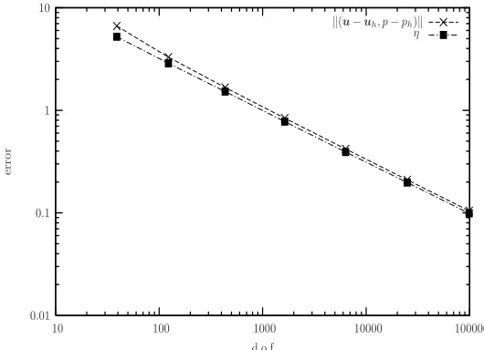
In order to test our a posteriori error estimator in Figure 1 we depict the error, in the norm defined in (2.4), and the estimator ˜ηH as h→0. We can observe

that both values are in good accordance, which is confirmed in Table 1 where we show the effectivity index

Ei :=

˜

ηH

k(u₋u_h, p₋ph)k

,

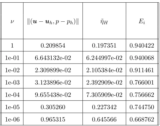
which remains bounded as h _→ 0. Finally, in order to study the sensitivity of the effectivity index as ν → 0, we present in Table 2 the behavior of ˜ηH

and k(u₋u_h, p−ph)k for a fixed mesh and for ν = 1,10−1, . . . ,10−6. We

observe that, as was predicted by Theorem 16, the estimator ˜ηH follows the

same pattern of k(u₋uh, p−ph)k, and hence, the effectivity index remains

η

k(u−uh, p−ph)k

d.o.f

e

rr

o

r

100000 10000

1000 100

10 10

1

0.1

0.01

Fig. 1. Exact error and the a posteriori error estimate.

d.o.f _k(u₋uh, p−ph)k η˜H Ei

39 6.641955 5.216376 0.785367 123 3.292848 2.873238 0.872569 435 1.671618 1.523188 0.911205 1635 0.838908 0.775193 0.924050 6339 0.419710 0.392412 0.934960 24963 0.209854 0.197351 0.940422 99075 0.104919 9.900770e-02 0.943655 Table 1

ν _k(u₋uh, p−ph)k η˜H Ei

1 0.209854 0.197351 0.940422 1e-01 6.643132e-02 6.244997e-02 0.940068 1e-02 2.309899e-02 2.105384e-02 0.911461 1e-03 3.123896e-02 2.392909e-02 0.766001 1e-04 9.655438e-02 7.305909e-02 0.756662 1e-05 0.305260 0.227342 0.744750 1e-06 0.965315 0.645566 0.668762 Table 2

Sensitivity of the estimator toν.

6.1.2 The lid-driven cavity problem

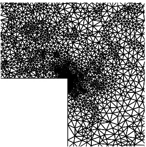
For this case we use the same domain as in previous section, we setf =0, and the boundary conditionsu=0on [{0} ×(0,1)]∪[(0,1)× {0}]∪[{1} ×(0,1)] and u = (1,0)t _{on (0,1)× {1}. We show in Figure 2 the initial mesh and}

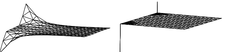
the adapted one obtained using our error estimate. In Figure 3 we depict the discrete pressure field obtained using the initial and adapted meshes where we note the improvement in the quality of the computed solution since the singular nature of the pressure is better captured in the adapted mesh.

Fig. 3. The pressure in the initial and adapted meshes.

6.1.3 The backward facing step problem

This test case is posed on the backward facing step configuration. The step is located at (x, y) = (2.5,0), the entry of the channel is at x = 0 and the exit of the channel at x= 22. The channel width is 1 at entry and 2 at exit. The boundary conditions are inflow parabolic profiles and free outflow. We assume f =0. In this case a singularity arises at the step from the re-entrant corner. Hence we can expect the meshes to be locally refined around the corner. In Figure 4 we depict the initial mesh, and in Figure 5 we show a zoom of the adapted mesh where we can observe the local behavior of the adapted mesh. Isovalues of the vertical component of the velocity are depicted in Figure 6 for both meshes. We remark the improvement in the quality of the discrete solution if we use the adapted mesh.

Fig. 5. A zoom, near the singularity, of the adapted mesh.

Fig. 6. A zoom, near the singularity, of the vertical velocity in the initial and the adapted meshes.

6.2 The generalized problem (σ₆= 0)

6.2.1 An analytical solution

For this test case we consider Ω = (0,1)_×(0,1), and with the aim of testing our approach using non-polynomial solutions, we set f such that the exact solution of our generalized Stokes problem is given by

u1(x, y) = sin(πx) sin(πy), u2(x, y) = cos(πx) cos(πy),

p(x, y) = 150(x−0.5)(y−0.5).

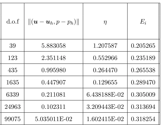
the same kind of information plus the effectivity index. Note that this case is not covered by our theoretical results since condition (F) is not satisfied. Nevertheless, the exact error follows the same pattern of our a posteriori error estimator.

η

k(u−uh, p−ph)k

d.o.f

e

rr

o

r

100000 10000

1000 100

10 10

1

0.1

0.01

Fig. 7. Exact error and the a posteriori error estimate (ν = 1 andσ = 1).

d.o.f _k(u₋uh, p−ph)k η Ei

39 5.883058 1.207587 0.205265 123 2.351148 0.552966 0.235189 435 0.995980 0.264470 0.265538 1635 0.447907 0.129655 0.289470 6339 0.211081 6.438188E-02 0.305009 24963 0.102311 3.209443E-02 0.313694 99075 5.035011E-02 1.602415E-02 0.318254 Table 3

η

k(u−uh, p−ph)k

d.o.f

e

rr

o

r

100000 10000

1000 100

10 100000

10000

1000

100

10

1

0.1

0.01

Fig. 8. Exact error and the a posteriori error estimate (ν = 1 and σ= 106).

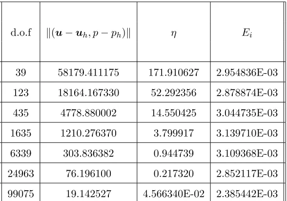
d.o.f _k(u₋uh, p−ph)k η Ei

39 58179.411175 171.910627 2.954836E-03 123 18164.167330 52.292356 2.878874E-03 435 4778.880002 14.550425 3.044735E-03 1635 1210.276370 3.799917 3.139710E-03 6339 303.836382 0.944739 3.109368E-03 24963 76.196100 0.217320 2.852117E-03 99075 19.142527 4.566340E-02 2.385442E-03 Table 4

Error, a posteriori error estimator and effectivity index (ν = 1 and σ= 106_).

6.2.2 The lid-driven cavity problem

Fig. 9. Initial and final adapted meshes.

0 0.1 0.2 0.3 0.4 0.5 0.6 0.7 0.8 0.9 1 -0.1

0 0.1 0.2 0.3 0.4 0.5 0.6 0.7 0.8 0.9 1

Fig. 10. A cross section of the tangential velocity atx= 1₂.

7 Concluding remarks

An adaptive finite element scheme for the generalized Stokes equation has been introduced and analyzed. This scheme is based on a stabilized finite element method combined with an a posteriori error estimator. This error estimator is cheap and easy to calculate once we have chosen the bubble function spaces to be used. The equivalence between the estimator and the finite element error has been proved using a general hypothesis on the auxiliary bubble function spaces, thus avoiding the use of a saturation assumption, and we have provided a concrete pair of bubble spaces satisfying this requirement.

de-pending on the physics of the problem, we remark that, for the pure Stokes problem, they provide equivalence constants which are independent of the vis-cosity. We also note that this dependence arises from the auxiliary problem posed on the continuous setting, and not from the hierarchical approach.

Finally, it is worth remarking that, even if the basic idea is closely related to the idea from [3] (see also [18]), our presentation is more general and the actual error estimator is quite different, and easier to compute. The extension of this idea to the Oseen and to the fully nonlinear Navier-Stokes equations will be the subject of future research.

A The proof of Lemma 13

First, we give the following result concerning the stabilization parameterδT.

Lemma 18 Let T ∈ Th and let δT be given by (4.9). Then, the following

estimates hold

ν δT ≤

1 12h

2

T , (A.1)

σ δT ≤min{hTν−1/2σ1/2,1}. (A.2)

PROOF. In order to prove the first estimate we use (4.9) and (4.10) to obtain

δT ≤

h2

T

4ν/mk ≤

1 12ν

−1_h2

T ,

estimate which is valid independently of the value of σ. Second estimate is obvious ifσ = 0, hence we will suppose from now on that σ >0. First, we use (4.9) to get

σ δT ≤

1 max{λT,1}

≤1. (A.3)

On the other hand, we know from (A.1) that δT ≤ ₁₂1ν−1h2T, and then

σ δT ≤

1 12h

2

T ν−1σ . (A.4)

Taking then the geometric mean of (A.3) and (A.4), we have

σ δT ≤

1

√

12hT ν

−1/2_σ1/2_{. (A.5)}

Now, we are ready to prove Lemma 13. We will prove the result only for the case σ >0, the other one being completely analogous. From the definition of

R1

h, using (4.8) with qh = 0, we have

R1h(vh) =

Z

Ωf·vh−a(uh,vh)−b(vh, ph) =

X

T∈ Th

Z

T δT RT (σvh−ν∆vh).

Next, from Cauchy-Schwarz’s inequality, (3.2) and (A.1), we obtain

νδT

Z

T

R_T ∆v_h≤νδT

Z

T|

R_T||∆v_h|

≤h

2

T

12kRTk0,Tk∆vhk0,T

θT kRTk0,Tkvhka,T.

On the other hand, using (A.2), Cauchy-Schwarz’s inequality and the defini-tion of θT we obtain

σ δT

Z

T

R_Tv_h≤min{ν−1/2σ1/2hT,1} kRTk0,Tkvhk0,T

≤θT kRTk0,Tkvhka,T,

and the result follows.

B Bubble function spaces satisfying (LBB) condition

For each element T ∈ Th we define the element bubble function bT by

bT := 27

Y

x∈N(T)

λx, (B.1)

where λx denotes the barycentric coordinate associated to node x. Following

Verf¨urth [22], let Tb be the standard reference element, of vertices (1,0),(0,1) and (0,0). Given any number α ∈ (0,1] let us denote by Φα : R2 → R2 the

transformation which maps (x, y) onto (x, αy). Let

b

Tα:= Φα(Tb),

and let us denote by ˆλ1,α,λˆ2,α and ˆλ3,α its barycentric coordinates (see Figure

(0,0) (1,0)

ˆ

T

(0,1)

(1,0) (0, α)

(0,0)

ˆ

Tα

ˆ

λ1,α ˆ

λ2,α

Φα( ˆT)

ˆ

λ3,α

Fig. B.1. TrianglesTband Tbα.

Set

b_{F ,αb} :=

    

4 ˆλ3,αλˆ1,α on Tbα,

0 on Tb_\Tbα,

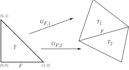
where Fb:=_{(t,0) _∈R2 _{: 0 ≤ t ≤1}. Let F ∈ EΩ and let us denote by T1, T2}

two triangles which have F in common. Let GF,i, i = 1,2, be the orientation

preserving affine transformation which maps Tb onto Ti and Fb onto F (see

Figure B.2).

(0;0) (0;1)

(1;0) ^

T

^ F

T 1

F

T 2 G

F;2 G

F;1

Fig. B.2. Affine transformationGF,i,i= 1,2.

Set

bF,α:=

    

b_{F ,αb} ◦G−_F,i1 on Ti, i= 1,2,

0 on Ω_\ωF.

(B.2)

Let ˆΠ := {(x,0) : x∈ R_{} and let ˆQ :} R2 _{→ Π be the orthogonal projection}ˆ

fromR2 _{to ˆΠ. We introduce the lifting operator ˆPˆ}

F :Pk( ˆF)→Pk( ˆT) by

ˆ

P_Fˆ(ˆs) = ˆs◦Q.ˆ

We define the lifting operator PF,Ti :Pk(F)→Pk(Ti) by

PF,Ti(s) = ˆP_Fˆ(s◦GF,i)◦G −1

F,i.

Using these notations, we can define a lifting operator

s_∈P_{k(F)−→PF(s) :=}

    

PF,T1(s) in T1,

PF,T2(s) in T2,

and, for s= (s1, s2)∈Pk(F)2, we denote

P_F(s) = (PF(s1), PF(s2)).

Finally, for allF _{∈ E}Ω let αF be the positive parameter given by

αF:=

    

min_{ν1/2_σ−1/2_h−1

F ,1} , σ >0,

1 , σ= 0.

Theorem 19 Let k_∈N_{. For all σ≥0, the following estimates hold}

kv_k2_0,T(v, bTv)T ,

ks_k2_0,F(s, bF,αFs)F,

kbT vka,TθT−1kvk0,T, (B.3)

kbF,αF PF(s)ka,ωF θ −1

F ksk0,F, (B.4)

for all T _{∈ T}h, F ∈ EΩ, and every polynomial v, s of degree k defined in T

and F, respectively.

PROOF. The first two inequalities are proved (for the scalar case) in [22], Lemma 3.3. To prove the latter ones, let us first suppose that σ > 0. Using the inverse inequality (3.3) and the fact that bT ≤1,

kbT vk2a,T=νk∇(bT v)k20,T +σkbT vk20,T

(ν h−_T2+σ)_kv_k2_0,T

σ(ν σ−1h_T−2+ 1)_kv_k2_0,T

σ max_{ν1/2σ−1/2h−_T1,1_}2_kv_k2_0,T

σ min_{ν−1/2σ1/2hT,1}−2kvk20,T,

kbF,αF PF(s)k 2 0,ωF =

X

Ti⊂ωF

kbF,αF PF(s)k 2 0,Ti

X

Ti⊂ωF

h2TikbF ,αb F ˆ

P_Fˆ(ˆs)k2_0,Tb (B.5)

Now, Lemma 3.3 in [22] applied to the vectorial case leads to

kb_{F ,αb}

F ˆ

P_Fˆ(ˆs)k_0,Tb√αFksˆk_0,Fb, (B.6)

kc∇(b_{F ,αb}

F ˆ

P_Fˆ(ˆs))k_0,Tb

s

αF +

1

αF k

ˆ

s_k0,Fb, (B.7)

and hence, using (B.5),(B.6) and the mesh regularity, we obtain

kbF,αF PF(s)k 2

0,ωF αFh 2

F kˆsk2_0,Fb αFhF ksk20,F.

Moreover

σ hFαF = ν1/2σ1/2 min{1, ν−1/2σ1/2hF}

≤ ν1/2σ1/2 min{1, ν−1/2σ1/2hF}−1 = θF−2,

and then

σkbF,αF PF(s)k 2

0,ωF θ −2

F ksk20,F. (B.8)

On the other hand, from (B.7) andαF ≤1, it holds

k∇(bF,αFPF(s))k 2 0,ωF =

X

Ti⊂ωF

k∇(bF,αFPF(s))| 2 0,Ti

k∇ˆ(ˆbF,αFPˆ_Fˆ(ˆs))k 2 0,Tb

α−_F1ksˆ_k2 0,Fb

h−_F1α−_F1ks_k2_0,F,

and using that ν h−_F1α−_F1 = θ−_F2, we obtain

νk∇(bF,αF PF(s))k 2

0,ωF θ −2

F ksk20,F . (B.9)

Hence, the result for σ >0 follows from (B.8) and (B.9). The proof for σ= 0 follows in an analogous way. 2

In order to satisfy the (LBB) condition we need to impose the following con-dition on f:

(F) f is a piecewise polynomial function, i.e., there exists a positive integer

t such that

f _{∈ {}g_∈L2_(Ω)2 _{: g|}

Remark 20 One possibility to overcome condition (F) above is to split the error between the error due to data approximation and the error due to the numerical method, as it has been done, for instance, in [1]. In any case, we

remark that, since the degree t of the polynomial from condition (F) is not

upper bounded, the error between f and its local projection onto the piecewise

polynomial space may be seen as a higher order term.

Next, we define the following bubble function spaces:

Hb_T :=_h{bTRT}i ∀T ∈ Th,

Hb_F :=h{bF,αF PF(RF)}i ∀F ∈ EΩ,

wherebT and bF,αF are the bubble functions given by (B.1) and (B.2), respec-tively.

Remark 21 We remark that this definition of bubble functions allows us use any polynomial order to approximate the velocity and the pressure. In fact,

for every k, l _≥ 1 the bubble function bTRT belongs to Pmax{t,k,l−1}+3(T) and

bF,αF PF(RF) belongs to Pk+1(T). Hence, H

b

T and HbF are not subspaces of

H_h.

Since bT RT ∈HbT, using Theorem 19 we arrive at

sup BT∈H b T

(RT,BT)T

θTkRTk0,T aT(BT,BT)1/2 ≥

(RT, bT RT)T

θT kRTk0,TaT(bT RT, bT RT)1/2

kRTk

2 0,T

θT kRTk0,T θT−1kRTk0,T

β .

The same analysis may be carried out for every F ∈ EΩ. In fact, we have

sup BF∈H b F

(R_F,BF)F

θF kRFk0,FaωF(BF,BF) 1/2

≥ (RF, bF,αF RF)F

θFkRFk0,FaωF(bF,αF PF(RF), bF,αF PF(RF)) 1/2

kRFk

2 0,F

θFkRFk0,F θF−1kRFk0,F

References

[1] M. Ainsworth. A posteriori error estimation for lowest order Raviart-Thomas mixed finite elements. Technical Report 23, University of Strathclyde, Department of Mathematics, 2006.

[2] M. Ainsworth and J. T. Oden. A posteriori error estimation in finite element analysis. John Wiley & Sons, New York, 2000.

[3] M. Ainsworth and J.T. Oden. A posteriori error estimators for the Stokes and Oseen equations. SIAM J. Numer. Anal., 34:228–245, 1997.

[4] R. Araya, G.R. Barrenechea, and F. Valentin. A stabilized finite-element method for the Stokes problem including element and edge residuals. IMA J. Numer. Anal., 27(1):172–197, 2007.

[5] R. Araya, E. Behrens, and R. Rodr´ıguez. An adaptive stabilized finite element scheme for the advection-reaction-diffusion equation. Appl. Num. Math., 54:491–503, 2005.

[6] R. Araya, A. Poza, and E.P. Stephan. A hierarchical a posteriori error estimate for an advection-diffusion-reaction problem. Math. Models Methods Appl. Sci., 15(7):1119–1139, 2005.

[7] R.E. Bank and B.D. Welfert. A posteriori error estimators for the Stokes problem. SIAM J. Numer. Anal., 28:591–623, 1991.

[8] G. Barrenechea and F. Valentin. An unusual stabilized finite element method for a generalized Stokes problem. Numer. Math., 92(4):653–677, 2002.

[9] F. Brezzi and M. Fortin. Mixed and hybrid finite element methods. Springer-Verlag, New York, 1991.

[10] P. Cl´ement. Approximation by finite element functions using local regularization. R.A.I.R.O. Anal. Numer., 9:77–84, 1975.

[11] E. Dari, R. Dur´an, and C. Padra. Error estimators for nonconforming finite element approximations of the Stokes problem. Math. Comp., 64:1017–1033, 1995.

[12] W. D¨orfler and M. Ainsworth. Reliable a posteriori error control for nonconformal finite element approximation of Stokes flow. Math. Comp., 54(252):1599–1619, 2005.

[13] H. Elman, D. Silvester, and A. Wathen. Finite elements and fast iterative solvers: with applications in incompressible fluid dynamics. Oxford University Press, New York, 2005.

[14] A. Ern and J.-L. Guermond. Theory and practice of finite elements. Springer-Verlag, New York, 2004.

[16] T.J.R. Hughes and L.P. Franca. A new finite element formulation for computational fluid dynamics: VII. The Stokes problem with various well-posed boundary conditions: Symmetric formulations that converge for all velocity/pressure spaces. Comput. Methods Appl. Mech. Engrg., 65(1):85–96, 1987.

[17] V. John. A numerical study of a posteriori error estimators for convection-diffusion problems. Comput. Methods Appl. Mech. Engrg., 190:757–781, 2000. [18] D. Kay and D. Silvester. A posteriori error estimation for stabilized mixed

approximations of the Stokes equations. SIAM J. Scientific Computing, 21:1321–1336, 1999.

[19] J.R. Shewchuk. Delaunay refinement algorithms for triangular mesh generation. Computational Geometry: Theory and Applications, 22(1–3):21–74, 2002. [20] R. Verf¨urth. A posteriori error estimators for the Stokes problem. Numer.

Math., 55:309 – 325, 1989.

[21] R. Verf¨urth. A posteriori error estimators for the Stokes problem II. Non-conforming discretizations. Numer. Math., 60:235 – 249, 1991.