Designing optimal low-thrust gravity-assist trajectories using space-pruning and a multi-objective approach

Designing Optimal Low Thrust Gravity Assist Trajectories

Using Space Pruning and a Multi-Objective Approach

Oliver Sch¨

utze

_{, Max Vasile}

_{, Oliver Junge}

_,

Michael Dellnitz

_{, and Dario Izzo}

1

_{(corresponding author)}

_{CINVESTAV-IPN, Computer Science Department}

Mexico D.F. 07300, MEXICO

email:

[email protected]

2

_{University of Glasgow}

Department of Aerospace Engineering (

http://aero.gla.ac.uk/

James Watt South Building

G12 8QQ, Glasgow,UK

email:

[email protected]

_{Technische Universit¨}

_{at M¨}

_unchen

Zentrum Mathematik / M3

Boltzmannstr. 3

D-85747 Garching, GERMANY

email:

[email protected]

_{University of Paderborn}

Institute for Industrial Mathematics

D-33098 Paderborn, Warburger Strasse 100, GERMANY

email:

[email protected]

5

_{European Space Agency}

Advanced Concepts Team (

http://www.esa.int/act

)

ESTEC, DG-PI, Keplerlaan 1

2201 AZ Noordwijk - THE NETHERLANDS

email:

[email protected]

(August 2007)

Keywords:space mission design, low-thrust gravity assist transfers, pruning techniques, multi-objective optimisation

1

Introduction

NASAs Deep Space 1 and recently ESAs SMART-1 have shown the effectiveness of low-thrust systems as primary propulsion devices. Such new scenarios make the task of mission analysts more difficult than ever. In fact, the design of a low-thrust transfer generally requires the solution of an optimal control problem, which has no general solution in closed form. Different methods have been developed to tackle these trajectory design problems. However, all of them need to be initialised with a first guess solution. The generation of a suitable first guess turns out to be a tricky and quite time consuming task. Studies on the generation of first guess solutions for low-thrust transfers, date back to the late nineties with the works of Coverstone et al. (4, 16), where multi-objective genetic algorithms were first used to compute first guess solutions for an indirect method. The derivation of approximating analytical solutions was addressed in the works of Markopoulos (10), Bishop and Azimov (1, 2). Inspired by the work of Tanguay (20), Petropoulos and Longuski (15) proposed a shape-based approach, which represents the trajectory (connecting two points in space) with a particular parameterised analytical curve (or shape) and computes the control thrust necessary to satisfy the dynamics. Although the resulting trajectory is not the actual solution of an optimal control problem, by tuning the shaping parameters it is possible to generate solutions, which are sufficiently good to initialise a more fine optimisation process. More precisely, in the work by Petropoulos, a thrust arc is represented by an analytical curve, known as

exponential sinusoid, which consists of a five parameter shape in polar coordinates. This shape is suitable for the approximation of planar motion, and the reduced number of shaping parameters does not allow to satisfy all the possible boundary conditions on position, velocity, time of flight and magnitude of the control acceleration; for 3D problems the propellant consumption for out of plane motion is only estimated. By implementing the exponential sinusoid trajectory model in the software code STOUR, Petropoulos and Longuski extended their systematic search for optimal ballistic MGA transfers to the global solution of Low-Thrust Gravity Assist (LTGA) transfers (11, 15, 13). Recently, it has been shown that whenever a Multiple Gravity Assist (MGA) optimisation problem is characterised by a simple ∆v-matching for the swing-bys and no deep-space manoeuvres are present, there exists a polynomial-time algorithm (with small exponent) that provides an efficient solution to the problem (13). Namely a branch and prune technique exists, the complexity of which is quartic with respect to dimensionality, i.e. in the number of swing-bys, and cubic in the resolution of the discretisation of the time variable. Space pruning techniques are incremental algorithms which allow pruning out infeasible regions from a given domain (or space), which is typically huge compared to the feasible set, measured by its volume. Pruning techniques have been used for decades as part of various deterministic algorithms (14), from branch and prune algorithms applicable to general black-box problems to algorithms built on specific problems, such as the one in (13). Pruning heuristics simply select from the domainD, which is often neatly defined by box constraints, a collectionC of disconnected subsetsSi⊂Dof different shape and size. Thus, the success of the pruning techniques highly depends on the way they are integrated into the entire optimisation process.

The results in (13) are particularly interesting for two reasons: the authors demonstrated that, by exploiting problem characteristics, the search space for a particular model of MGA trajectories, could be pruned very efficiently; pruning the search space increased significantly the probability of finding a good local optimum with a stochastic based global optimisation method (in (13) the authors used an implementation of Differential Evolution). Since the pruning process was particularly efficient, the overhead in the computation cost due to the application of the pruning plus the global search was largely compensated by the increase in the reliability of the search process. Here it is understood that a search process is reliable if a given solution can be found with high probability over a number of times that the process is run.

manoeuvres considered. Further, one possible way to use the output setCto tackle the

multi-objective optimisation problem (MOP) under consideration (i.e., minimisation of flight time and fuel consumption) will be shown. To be more precise, multilevel subdivision techniques will be used, which are state of the art for the numerical treatment of moderate dimensional and

continuous MOPs and which can cope with disconnected domains. The resulting process—i.e., pruning and subdivision—is suitable to solve such MLTGA problems efficiently and is competitive with other existing methods.

In (13) the pruning algorithm was devised to address specifically MGA problems with a particular structure. The algorithm is therefore problem dependent and fully exploits the characteristics of the problem.

In this paper the heuristics proposed in (13) to tackle MLTGA problems will be extended. Furthermore in (13) the pruning of the solution space was intended as a way to improve the search of a stochastic-based global optimiser for single objective problems. In this paper, instead, the pruned space is used to improve the search of a multi-objective algorithm and in particular it will be shown how to improve the identification of the global Pareto front for an MLTGA problem. The remainder of this paper is organised as follows: in Section 2 the background required for understanding the work is stated. Section 3 proposes an incremental pruning algorithm for MLTGA problems and its complexity is analysed in Section 4. Section 5 deals with the numerical treatment of the multi-objective trajectory design problem, in Section 6 some numerical results are presented, and finally conclusions are drawn in Section 7.

2

Background

In this section the required background for the understanding of the sequel is stated: the concept of multi-objective optimisation is introduced, the trajectory design problem is stated, and finally the subdivision techniques are described which will be used to attack the resulting problems.

2.1

Multi-Objective Optimisation

In a variety of applications in industry and finance a problem arises that several objective functions have to be optimised concurrently. One important feature of these problems is that the different objectives typically contradict each other and therefore certainly do not have identical optima. Thus, the question arises how to approximate one or several particular ‘optimal compromises’ or how to compute the entire set of optimal compromises – thePareto set– of thismulti-objective

optimisation problem(MOP). For the solution of both problems there already exists a huge variety

of efficient algorithms (see e.g. (12), (5) and references therein).

Mathematically speaking, an MOP can be stated in its general form as follows:

min

x∈S{F(x)}, S={x∈

n_{:h(x) = 0, g(x)≤0},}

whereF is defined as the vector of the objectives, i.e.

F: n→ k, F(x) = (f1(x), . . . fk(x)),

withf1, . . . , fk: n→ ,h: n→ m,m≤n, andg: n→ q. A vectorv∈ kis said to be

dominatedby a vectorw∈ k_{ifwi≤vifor alli∈ {1, . . . , k}andv6=w. A vectorvis called}

nondominatedwith respect to a setP, if none of the vectorsp∈P dominatev.

A pointx∈ Sis called optimal orPareto optimal, ifF(x) is not dominated by any vector

2.2

The Exponential Sinusoid

It is here proposed to use a particular model for multiple gravity assist low-thrust trajectories (MLTGA). Low-thrust arcs are modeled through a shaping approach based on the exponential sinusoid proposed by Petropoulos et al.(15). The spacecraft is assumed to be moving in a plane subject to the gravity attraction of the Sun and to the control accelerationF_{= [}Fcosα, Fsinα]T

of a low-thrust propulsion engine. The dynamic equations governing the motion of the spacecraft can be written in polar coordinates as follows:

¨

r−rθ˙2+ µ

r2 =Fsinα

1

r d dt(r

2_{θ˙) =Fcosα}

whereαis the thrust steering angle measured clockwise from the axis perpendicular torin the direction of motion. For this particular dynamics Petropoulos proposed to use the following shaping function for the radius as a function of the polar angleθ.

r=k0ek1sin(k2θ+φ)

Then, if the thrust vector is aligned with the velocity vector, the flight path angleγand the thrust steering angleαare equal. Ifγ=α, the thrust history and the polar angle history are uniquely determined and the control acceleration is given by:

F= µ

r2

tanγ

2 cosγ »

1 tan2_γ+k1k2

2s+ 1

− k

2

2(1−2k1s)

(tan2_γ+k1k2 2s+ 1)2

–

(2.1)

with the time variation of the true anomaly given by:

˙

θ2₌“µ r3

” ₁

tan2_γ+k1k2 2s+ 1

(2.2)

and the flight path angle given by:

tanγ=k1k2cos(k2θ+φ) (2.3)

withs= sin(k2θ+φ). Now, by solving the following integral:

∆t=

Z _dθ

r“_µ r3

” 1 tan2_γ+k

1k22s+1

(2.4)

one can compute the actual time of flight.

The exponential sinusoid expresses the variation of the radius as a function of the polar angleθand depends on three shaping parametersk0, k1, k2 plus a phase parameterφ. By fixing the initial and final radius forθ= 0 andtheta= ¯θrespectively:

r1=k0ek1sin(φ)

r2=k0ek1sin(k2θ+φ)¯

two of the three parameters can be computed as a function of the others (8).

The two position radii and the angular difference ¯θbetween the departure and the arrival points can be computed from the ephemerides of the departure and arrival planets or other celestial bodies (in this work analytical ephemerides are used). In this case it is normally required that the transfer trajectory going from one planet to the other is flown in a given timeT. This implies that the actual time of flight must be equal to the required time of flight in order to have a physical solution:

∆t−T= 0 (2.6)

If now this time constraint is solved a third parameter can be determined and the exponential sinusoid becomes a single valued function (for more details on the solution of 2.6 please refer to (8)). In this form, given the transfer time and the two position vectors at the beginning and at the end of the transfer the velocities at the two extremal points and the thrust profile can be computed. Since only one shaping parameter is free it is not possible to optimise the value of the velocities at the boundaries plus the thrust profile but the problem is equivalent to the Lambert’s problem for conic arcs.

Furthermore some analysis (15) reveals that the exponential sinusoid gives physical solutions wheneverk1k22<1. This limit will be used in the remainder of this paper to limit the values of the

shaping parameterk2.

2.3

Gravity Assist Model for the Exponential Sinusoid

Gravity assist manoeuvres are modeled with a linked-conic approximation: the manoeuvre is instantaneous (i.e., no variation in the position of the spacecraft) and produces a deflection of the planetocentric velocity vector, the planet is reduced to a point mass with no gravity, the deflection angleβswingis a function of the mass of the planet and of the incoming velocity, such that:

e

vT_inev_out=−ev2_icosβswing (2.7)

and

βswing= 2 arccos` µp

e v2

inrp+µp ´

(2.8)

whereµpis the gravity constant of the swing-by planet,ev_inandev_{outare the planetocentric}

incoming and outgoing velocity vectors andrpis the radius of the pericentre of the swing-by hyperbola.

Since the value of the velocities at the boundaries is not completely free, given an incoming velocity vector it is not possible, in general, to match every possible outgoing velocity vector.

A match can be obtained by inserting a ∆V correction at the pericentre of the hyperbola of the swing-by. This model will be called powered swing-by model or powered swing-by in the following. Modeling gravity manoeuvres through powered swing-bys has a very important property: it decouples the transfer arcs one from the other. In fact each transfer arc can be computed independently from the others once the departure and arrival times of a transfer arc are defined. Than, any pair of arcs can be matched through a ∆vmanoeuvre. As will be shown in the remainder of the paper, this important property of this specific trajectory model, allows to device an algorithm with polynomial complexity that can incrementally prune the search space.

2.4

Problem Formulation

ForN+ 1 celestial bodies, a sequence of thrust legs is then assembled to all the others through a sequence of powered swing-bys. Each thrust leg is modeled through a shape-based method based on exponential sinusoids (15, 8), and the first objective is given as:

minimise: J(y)

subject to: rp≥rmin (2.9)

the complete solution vector is then defined as follows:

y= [t0, T1, k2,1, n1, ..., Ti, k2,i, ni, ..., TN, k2,N, nN]T _(2.10)

wherek2,iis the i-th shaping parameter for the exponential sinusoid andnithe number of

revolutions around the Sun. The objective functionJis then defined as follows:

J= 1−exp

„

−

„

∆VGA+ ∆V0 g0Isp1

+∆VLT

g0Isp2 ««

(2.11)

where ∆VGAis the sum of all the ∆V s(variation in velocity) required to correct every gravity assist manoeuvre, ∆V0 is the departure manoeuvre, while ∆VLT is the sum of the total ∆V of each

low-thrust leg. The two specific impulsesIsp1 andIsp2are respectively for a chemical engine and for a low-thrust engine andg0is the gravity acceleration on the surface of the Earth.

For the tests in this paper, the valuesIsp1= 315s andIsp2= 2500s are used. Note that, the computation of a transfer arc with the exponential sinusoid does not require the time history of the mass of the spacecraft. The time history of the mass would be required to compute the actual thrust profile along the transfer arc. The integration of 2.1, instead, gives directly the ∆vdue to the low-thrust propulsion.

The objective function 2.11 is particularly appealing because it has values ranging from 0, best transfer, to 1, worst transfer. In addition the impulsive ∆vand the low-thrust ∆vare weighted in such a way that the use of low-thrust is favorite with respect to the use of the impulsive

corrections. Note that, the scope of this paper is not to demonstrate the suitability of the exponential sinusoid model for the design of MLTGA trajectories but rather to demonstrate the effectiveness of the proposed pruning technique.

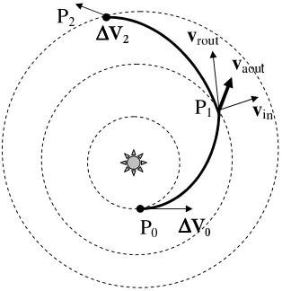
The overall process for the composition of an MLTGA trajectory with the exponential sinusoid model can be summarised with the following steps (see Fig. 1) :

• For each departure datet0andN legs with transfer timesT_{= [T1, ..., Ti, ..., TN]}T

• Compute a low-thrust arc through the exponential sinusoid model from planetito planeti+ 1 (see the transfer from A to B as an example in Fig. 1)

• Compute the incoming heliocentric velocity vectorv_{inand the corresponding planetocentric}

velocity vectorev_in

• Compute a low-thrust arc through the exponential sinusoid model from planeti+ 1 to planet

i+ 2 (see the transfer from B to C as an example in Fig. 1)

• Compute the required heliocentric outgoing velocity vectorv_{routand the corresponding}

required planetocentric velocity vectorev_rout

• Compute the achievable planetocentric outgoing velocity vectorev_{aoutwith pericenter radius}

rp≥rmin

• Ifve_aout6=v_{eroutcompute the matching ∆}Viat the pericentre of the hyperbola • Compute the launch impulsive manoeuvre ∆V0

• Compute the arrival impulsive manoeuvre ∆VN

• Compute the the low-thrust ∆VLT

• Compute the sum of all ∆V’s

The arrival at planeticorresponds to a timeti=ti−1+Ti, therefore the final time at the end of

required for every plane change is obtained through an impulsive manoeuvre at the boundaries of the low-thrust arc and included in ∆V0, ∆VN, or in the ∆VGA.

Figure 1. Composition of a whole MLTGA trajectory for the exponential sinusoid model

The second objective of the MOP which is addressed in this work is simply given by theflight time

tN−t0used for the selected trajectory. This objective is of great importance for the design process

since the transfer can take several years (see e.g. the examples in Section 6). Thus, the MOP under consideration reads as follows:

minimise:

( J(y)

tN−t0

subject to: rp≥rmin

(2.12)

2.5

Subdivision Techniques

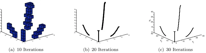
The subdivision techniques in (17), (7) have been primarily designed for MOPs without equality constraints. Algorithms of this type start with a compact subsetQ⊂ S of the parameter space, typically with one or moren-dimensionalboxes. Each box gets subdivided into a set of smaller boxes, and according to certain conditions it is decided which box could contain a part of the Pareto set and is thus interesting for further investigation. The other, unpromising boxes are discarded from the collection. This process, i.e., subdivision and selection, is performed on the current box collection until the desired granularity of the boxes is reached. The approach is of global nature, that is, in principle capable of detecting the entire set of Pareto points, see Fig. 2 for an example. Subdivision algorithms are very effective for the numerical treatment of moderate dimensional models, but, however, may become inefficient compared other approaches like e.g. evolutionary strategies for higher-dimensional models. To combine the strength of both approaches, a combination of subivision techniques with evolutionary strategies has been proposed in (19). Though it was not required to use this hybrid method for the numerical results presented in the sequel, it is an interesting candidate for the treatment of further (higher-dimensional) models. Note that the initial box collection—as well as any further collections—(a) can in principle consist of any number of boxes and that (b) the collection doesnothave to form one connected

0 10 20 30 40 0 10 20 30 40 0 5 10 15 20 25 30 35 40

(a) 10 Iterations

0 10 20 30 40 0 10 20 30 40 0 5 10 15 20 25 30 35 40

(b) 20 Iterations

0 10 20 30 40 0 10 20 30 400 10 20 30 40 x1 x2 x 3

(c) 30 Iterations

Figure 2. Application ofDS-Subdivisionon an MOPF:Q⊂

3_→

2_{, whereQis defined by}

box-constraints (see (7)).

3

LTGASP – Low Thrust Gravity Assist Space Pruning

In this section the LTGASP algorithm is proposed which is designed to efficiently detect and prune infeasible parts of the domain of a given MLTGA problem.

3.1

The MLTGA Problem Formulation

In order to be able to perform the pruning the numbers of revolutions in the design problem (2.12) have to be fixed. Thus, given an arbitrary butfixedsequence (n1, . . . , nN) of numbers of

revolutions the following problem is considered:

minimise:

( J(˜y)

tN−t0

subject to: rp≥rmin

(3.1)

where the solution vector ˜yis given by:

˜

y= [t0, T1, T2, . . . , TN, k2,1, . . . , k2,N],

and where the parameters have the following ranges:

t0∈ I0,

Ti∈ Ii, i= 1, . . . , N,

k2,i∈ Ik2,i, i= 1, . . . , N.

DefineIas the entire search space, i.e.

I:=I0×. . .IN× Ik2,1×. . .× Ik2,N. (3.2)

Introducing the map (analogue to (9))

defined by the component wise relationti=t0+Pi_j=0Tj, i= 0, . . . , N, and setting

I∗

:=f(I)× Ik2,1×. . .× Ik2,N (3.3)

problem (3.1) can be re-formulated as:

minimise:

( J(X)

tN−t0

subject to: rp(X)≥rmin,

(3.4)

which will be considered in the sequel. In the following, some notations are given which are helpful for the statement of the different pruning techniques. Every (feasible) trajectory from planetpi−1

to planetpiin the current setting is determined by the parametersti−1, ti,andk2,i. Given these

three values, denote the resulting trajectory frompi−1 topiby

T(ti−1, ti, k2,i).

Further, denote byD(I∗

i) andD(Ik2,i) the discretisations ofI

∗

i andIk2,i. Thus, the entire

discretised search space is given by

D(I∗

) =D(I∗

0)×. . .×D(IN∗)×D(Ik2,1)×. . .×D(Ik2,N).

3.2

The Pruning Techniques

In the following the pruning techniques are proposed which are used for the LTGASP algorithm. A pseudocode of all algorithms can be found in Appendix 1.

Initialisation.

i), i= 0, . . . , n, as valid as well as all trajectories

T(ti−1, ti, k2,i), ∀ti−1∈D(Ii∗−1), ti∈D(I

∗

i), k2,i∈D(Ik2,i), i= 1, . . . , N.

∆

V

_{constraining.}

algorithm in phasei. It works on the sampled spaceD(I∗

i−1)×D(I

∗

i)×D(Ik2,i) and prunes out all

those points corresponding to trajectories having a velocity change larger than a given budget ∆Vmax

i .

Algorithm1describes the ∆V pruning for the transfer from planetpi−1to planetpi, i. e. for phase i. Denote by ∆Vi(T) the velocity change required by a given trajectoryT.

Departure velocity constraining.

departure velocity (and thus the corresponding thrust required by the spacecraft) is larger than a given threshold.

Forward pruning.

search space volume of an MLTGA problem significantly. As a consequence many values of the arrival timetiin phaseibecome nonfeasible departure times in phasei+ 1. To be more precise: if there is no feasible trajectory that arrives at a planet on a given date because they have all been pruned out according to the various criteria introduced, then there will be no departures from that planet on that date. Thus, all the corresponding points will also be pruned.

Algorithm2describes the forward pruning from phaseito phasei+ 1 with respect toti∈D(I∗

Backward constraining.

Algorithm3describes the backward pruning from phasei+ 1 back to phaseiwith respect to

ti∈D(I∗

i).

Gravity assist maximum thrust constraint.

constraint prunes out the trajectories having a difference between incoming velocities of trajectories in phasei(denote this velocity byVi

end(T) for a given trajectoryT) and outgoing velocities of

trajectories in phasei+ 1 (denote byV_starti+1(T)) during a gravity assist larger than some threshold,

Av. This threshold has to be set separately for each gravity assist. Further, an appropriate tolerance,Lv, based on the Lipschitzian constant of the current phase plot has to be taken into account.

Algorithm4describes the gravity assist maximum thrust constraint pruning between phaseiand phasei+ 1.

Gravity assist angular constraint.

infeasible swing-bys from the search space on the basis of them being associated with a hyperbolic periapsis under the minimum safe distance for the given gravity assist body.

This is determined over every arrival date ¯ti∈D(I∗

i) as follows: for all incoming trajectories T(ti−1,ti, k¯ 2,i) and all outgoing trajectoriesT(¯ti, ti+1k2,i+1) check if the corresponding swing-by is

valid. In this case mark both incoming and outgoing trajectory as valid. Finally (i.e., after going through all arrival dates), all trajectories not marked as valid by this procedure will be pruned out. Algorithm5describes the gravity assist angular constraint pruning between phaseiand phasei+ 1.

Breaking manoeuvre constraint.

to add a constraint on the maximum breaking manoeuvre that a spacecraft can perform and prune out trajectories with an exceedingly high fuel demand.

3.3

The LTGASP Algorithm

Having stated the different pruning techniques the complete pruning algorithm can be formulated which is done in the followng.

Given an MLTGA problem (3.4), the LTGASP algorithm for the search space reduction reads as follows:

(0) perform the initialisation process.

(1) perform the ∆V pruning, departure velocity pruning as well as the forward pruning (one ‘phase shift’) for phase 1.

(2) forl= 2, . . . , n−1

(a) perform the ∆V pruning for phasel.

(b1) perform the backward pruning from phaseldown to phase 1. (b2) perform the forward pruning from phase 1 up to phasel+ 1.

(c) perform the gravity assist pruning for phasesl−1 andl. (d) perform the angular constraint pruning for phasesl−1 andl.

(3) perform all the pruning steps described in step (2) plus the breaking manoeuvre constraint for phasen.

Remarks 3.1_{(a) This is just one possible way to combine the different pruning techniques. Note}

that the steps 2(a), 2(b) and 2(c) can be interchanged, and that the outcome of the resulting pruning algorithm depends on this choice. However, since the angular constraint pruning is the most time consuming technique (see the numerical results in Section 6), it is logical to apply this technique at last in each phase. Further, it is also possible e.g. to apply the

(b) It has to be noted that the proposed pruning algorithm is of global nature, but does not

guarantee that parts of the feasible set arenotpruned out. This is due to the fact that the

algorithms work on a discretisation of the domain.

4600 4800 5000 5200 5400 5600 5800 6000 4800

5000 5200 5400 5600 5800 6000 6200 0 0.5 1 1.5

k2

1

t₀ t₁

(a) Phase 1

4800 5000 5200 5400 5600 5800 6000 6200 5000

5500 6000 6500 0 0.2 0.4 0.6 0.8

k2

2

t 1 t

2

(b) Phase 2

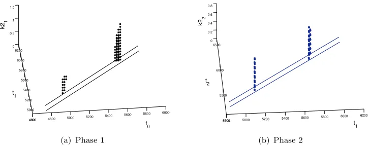
Figure 3. Possible resulting candidate set of the LTGASP algorithm for a two-phase sequence (Earth – Venus – Earth) consisting of two connected components in each phase. The straight lines

indicate the boundaries of the feasible subset inti−ti+1space,i= 0,1, which are given by the minimal (Tm,i) and maximal (TM,i) time of flight in each phase, i.e.,ti+1∈[ti+Tm,i, ti+TM,i].

4

Time and Space Complexity for the LTGASP Algorithm

This section determines the time and space complexity of the LTGASP algorithm. It will be shown that LTGASP scales quadratically in space and quintic in time with respect to the number of gravity assist manoeuvres considered. Since the focus is here on the order of the complexities for simplicity it can be assumed for the following analysis that the initial launch window and all phase times are the same.

4.1

Space Complexity

Consider a launch window, a mission phase time, and the range of thek0

2sdiscretised intolbins.

Thus, for the first phasel3_{Lambert problems have to be sampled. Since the number of possible}

times the planet may be arrived at in phasei, i= 1, . . . , ncan be assumed to be (i+ 1)l(see (9)) thei-th phase will require an amount of (i+ 1)l·l·l= (i+ 1)l3 _{Lambert function evaluations}

(given by the discretisations of the departure times, the time of flight andk2). This gives the series

O(n) =l3+ 2l3+. . .+nl3=l3n(1 +n)

2 .

Therefore, the amount of space required fornphases is only of orderO(n2_{), rather thanO(k}2n+1₎

for full grid sampling.

4.2

Time Complexity

The memory space requirement is directly proportional to the maximum number of Lambert problems that must be solved, and hence the time complexity of the sampling portion of the LTGASP algorithm must also be of the orderO(n2).

For the further time complexity analysis the following assumptions are made (see above):

|D(I∗

i)|= (i+ 1)l, i= 0, . . . , n,

|D(Ik_2,i)|=l, i= 1, . . . , n. (4.1)

∆

V

_{constraint complexity.}

assumption (4.1) it follows that|D(I∗

i−1)| · |D(Ii∗)| · |D(Ik2,i)| ≈i

2_l3_{. Thus, the time complexity}

applying the ∆V constraint isO(n3_{) with respect to the dimensionality andO(l}3_{) with respect to}

the resolution.

Forward and backward pruning complexity.

order ofi2_l3_{flops for one ‘phase shift’ (i.e., the pruning of the departure times for phasei+ 1 by}

analysing the data of phasei). Since for every phaseithere areisuch phase shifts (i.e., after the ∆V pruning of phaseiand after the backward pruning), for this pruning criterion an amount of

n X

j=1 j X

i=1 i2l3=l3

n X

j=1

j(j+ 1)(2j+ 1) 6

flops is required. Thus, the complexity of the forward pruning isO(n4_{) with respect to the}

dimensionality andO(l3) with respect to the resolution. Analogously, the complexity of the backward pruning is of the same order.

Gravity assist thrust constraint complexity.

2i2l3 operations. Thus, the time complexity applying the gravity assist thrust constraint isO(n3) with respect to the dimensionality andO(l3_{) with respect to the resolution.}

Gravity assist angular constraint complexity.

2i3_l5 _{operations. Thus, the time complexity applying the gravity assist angular constraint isO(n}4₎

with respect to the dimensionality andO(l5) with respect to the resolution.

Overall time complexity.

algorithm (the gravity assist angular constraint), is quintic with respect to the resolution and quartic with respect to the dimensionality.

5

Attacking the MOPs

Having performed the pruning techniques resulting in a candidate setCwhich typically has a much smallern-dimensional volume than the entire search spaceI(see Figure 3 for one example), the question arises how this information can be integrated efficiently into the optimisation process. Here one possible way is proposed to attack an MOP of the form (3.4) which involves the LTGASP algorithm presented above. Obviously, the pruning techniques have to be performed before the optimisation can start1_{. More interesting is how the setC, which can consist of up to hundreds of}

different connected components of different shape and size, can be utilised for the optimisation algorithm.

The authors of this work propose to proceed in the following way:

(1) Perform the LTGASP algorithm on the given setting. Denote the resulting candidate set byC. (2) Construct abox collectionRstarting fromCsuch that all boxes are mutually non-intersecting

and thatRcoversC’tightly’ (see discussion below).

(3) Perform the subdivision techniques described in Section 2 using collectionRas domain.

Before some numerical results can be presented, which is done in the next section, some remarks on the approach have to be made:

An-dimensional boxBcan be represented by boundsl, u∈

n_:

B=Bl,u={x∈

n_{:li≤xi≤ui∀i= 1, .., n}.}

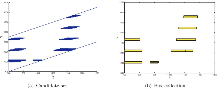
One way to construct a box collectionRwhich covers a candidate setCis by looking at the connected components of the logical three-dimensional matricesAiwhich correspond to thei-th phase: setajkl= 0 ifT(tj, tk, k2l) is detected as not valid for the underlying sequence, wheretjis

thej-th element of|D(I∗

i−1)|(analogous fortkandk2l); else setajkl= 1. The boxes can e.g. be

selected by taking the minimal and maximal coordinate values of each connected component (see Fig. 4 for an example). The correspondingn-dimensional boxes can be constructed on the basis of this sequence of three-dimensional boxes, and overlapping boxes have to be merged together. For a given setCthere does typically not exist one ‘ideal’ box collection as the following discussion shows: in order to speed up the computation, it is desired to keep the number of boxes small (since all boxes have to be evaluated). This can be done e.g. by merging ‘neighboring’ boxes together. However, since this increases the volume ofRthe probability of picking infeasible solutions in the run of the search procedure will increase which will in turn decrease its performance. To avoid this, smaller boxes can be considered which will in turn increase the number of boxes required to cover C. As an example consider the set in Fig. 5 (b), which consists of 57 connected components. If components which are merely separated by one discretisation step are merged together1 _the

resulting box collection consists of five boxes, which is probably the best trade off solution for this case.

For the stability of the transfer and due to the (long) resulting transfer times, up to date only few celestial bodies are involved for ‘real’ missions. Thus, the resulting domain of a given trajectory design problem can be considered to be low or moderate dimensional (say,≤15). The authors of this work have chosen to use subdivision techniques for the approximation of the Pareto sets since the algorithms can easily cope with the disconnected domain and since they have proven their efficiency on many applications so far (e.g., (7), (18)).

On the other hand, regarding the dimensionality of the models, certainly also other approaches can in principle serve to produce satisfying results. However, note that due to the particular structure of the domain an application is in most cases not straightforward. For instance, for multi-objective evolutionary algorithms (MOEAs, see e.g., (3)), the probably most widely used class of algorithms in this field, there does ad hoc exist no suitable cross-over operator since points from different connected components of the feasible set (or from different boxes) do typically not have similar characteristics. Further, a suitable penalisation strategy is also not straightforward.

6

Numerical Results

In this section some numerical results coming from two different settings are presented. All computations have been done on an Intel Xeon 3.2 Ghz processor using the programming language Matlab_.

1_{That is, if in the logical matrix described above elementsa}

j,k,lare set to 1 ifaj−1,k,l= 1 =aj+1,k,l,

700 800 900 1000 1100 1200 1300 800

1000 1200 1400 1600 1800 2000 2200

t 0

t1

(a) Candidate set

700 800 900 1000 1100 1200 1300

800 1000 1200 1400 1600 1800 2000 2200

t0 t1

(b) Box collection

Figure 4. Relaxation of the candidate set (right) by using boxes (right), which are much easier to handle for most optimisation algorithms.

6.1

Sequence EVMe

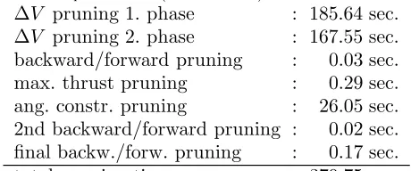
First the two-phase sequence Earth – Venus – Mercury (EVMe) is under consideration. Using the parameters shown in Table 1 (see Appendix 1) the LTGASP algorithm computes the candidate set displayed in Fig. 5. Here, the left upper limit on the arrival velocity has been kept very high to allow for many possible arrival conditions at Mercury. The computation took about seven minutes (see Table 2), a time which is equivalent to evaluate approximately 3,000 different trajectories (note that there is a strong relation between the time for the pruning process and the time for a function call since for the ∆V pruning single arcs of the trajectory have to be computed). The resulting box collection consists of 47 boxes with a total volume of 5.86·104_{. Since the volume of}

the entire search spaceI∗_{(see (3.3)) is 7.18·10}9_{, LTGASP pruned out 99.9992 percent of the}

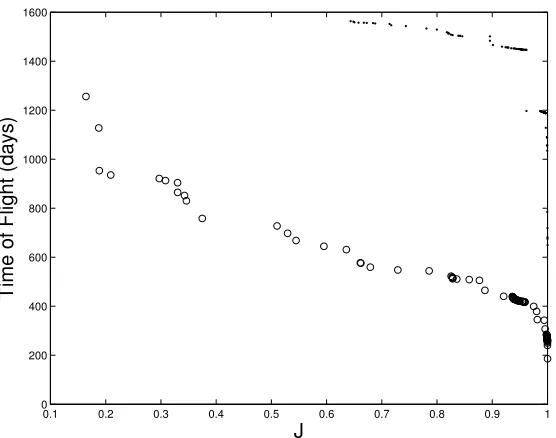
initial volume. Using the box collection as domain, the subdivision techniques described above obtained the Pareto front shown in Fig. 6 using a budget ofN= 50,000 function calls.

The huge diversity in the values of the front indicates that the multi-objective approach is indeed interesting for this mission: the total time of flight varies between 200 and 1200 days which makes a difference of nearly three years, and the mass fraction varies by more than 80 %, which is certainly a huge value as well.

In order to compare the results, the subdivision techniques have been used on the same problem but without the pruning (i.e., takingI∗

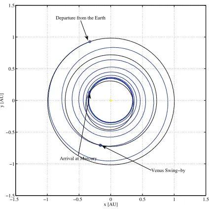
as domain). The results were not satisfying, even for much larger budgets for the number of function calls. Figure 5 shows one example forN= 50,000. The reason is that in the beginning of the algorithm relatively large boxes have to be evaluated where the fraction of the feasible set within these boxes are very small. Thus, it can easily happen that ‘good’ boxes—i.e., boxes containing a part of the Pareto set—are deleted by the algorithm. To prevent this, a huge amount of function calls has to be spent, at least in the early stages of the subdivision process. Thus, it is in this case the pruning which makes the subdivision algorithm work properly and is hence crucial for the efficiency of the proposed optimisation process. In 7 the trajectory plot is presented for the minimum mass solution, from the best Pareto front in Fig.6. The minimum time solutions, for this specific case, corresponds to trajectories that are not physically meaningful. Trajectories of this kind are possible in the model based on the exponential sinusoid, in particular if no strict restrictions on the thrust level are imposed.

6.2

Sequence EVEJ

700 800 900 1000 1100 1200 1300 800

1000 1200 1400 1600 1800 2000 2200

t₀

t1

(a) Phase 1

800 1000 1200 1400 1600 1800 2000 2200 1000

1500 2000 2500 3000 3500 4000

t₁

t2

(b) Phase 2

Figure 5. Numerical result of the LTGASP algorithm on the EVMe sequence.

0.1 0.2 0.3 0.4 0.5 0.6 0.7 0.8 0.9 1

0 200 400 600 800 1000 1200 1400 1600

J

Time of Flight (days)

Figure 6. The circles represent a Pareto front for the EVMe sequence obtained by the subdivision algorithm with a domainRwhich is a result of the pruning algorithm LTGASP. A solution of the

subdivision algorithm starting on the entire domainI∗

is given by the points.

spent which corresponds to approximately 3,000 function calls. The resulting box collectionR consists of eight boxes which have a total volume of 0.00006 percent of the volume of the entire search spaceI∗

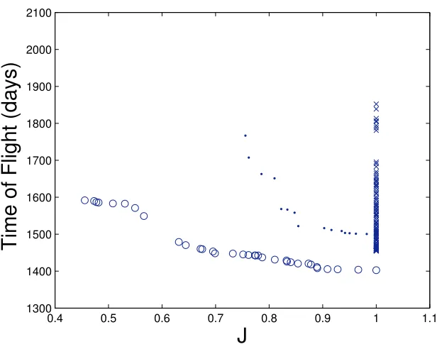
. Starting with this collection, the Pareto front displayed in Fig. 9 was obtained usingN= 60,000 function evaluations. Again, the function values along the obtained front differ significantly—400 days in the transfer time and 55% in the mass fraction—leading to a large variety for the decision maker.

For a comparison to other methods a random search procedure and the state-of-the-art

evolutionary algorithm NSGA-II (6) have been taken. For both approaches the entire search space

−1.5 −1 −0.5 0 0.5 1 1.5 −1.5

−1 −0.5 0 0.5 1 1.5

x [AU]

y [AU]

Arrival at Mercury Departure from the Earth

Venus Swing−by

Figure 7. Minimum mass solution, for the EVMe transfer, projected onto the ecliptic plane.

N= 100,000 function evaluations has been given. Two representative results can be seen in Fig. 9. Apparently, none of the two results can compete with the one coming from the combination of the pruning and the subdivision. This is due to the fact that the fraction of the feasible set withinI∗

is tiny as the relatively small volume ofRindicates. This might be also the reason that in this (very rare) case the random search operator outperforms NSGA-II. In such a case, a global search strategy seems to be more promising than any recombination strategy of inefficient or even useless trajectories which are obtained with a high probability, at least in the beginning of the run of the algorithm. This would change ifRwould be chosen as domain, but in that case it remains to define a suitable cross-over operator as discussed above. The result indicates that the approach proposed in this paper can cope—in contrast to existing ad hoc methods—efficiently with the given class of problems.

4600 4800 5000 5200 5400 5600 5800 6000

4800 5000 5200 5400 5600 5800 6000 6200

t

0

t1

(a) Phase 1

4800 5000 5200 5400 5600 5800 6000 6200

5000 5500 6000 6500

t

1

t2

(b) Phase 2

5000 5500 6000 6500

5500 6000 6500 7000 7500 8000

t

2

t3

(c) Phase 3

Figure 8. Numerical result of the LTGASP algorithm on the EVEJ sequence.

0.4 0.5 0.6 0.7 0.8 0.9 1 1.1 1300

1400 1500 1600 1700 1800 1900 2000 2100

J

Time of Flight (days)

Figure 9. Different Pareto fronts for the EVEJ sequence. The crosses represent one solution obtained by NSGA-II, the points a solution coming from random search, and the circles a result

obtained by pruning and subdivision.

7

Conclusions

In this work a bi-objective approach has been considered for the design of multi low-thrust gravity assist trajectories (minimisation of flight time and fuel consumption). For this, a novel way to tackle such problems, namely a combination of a space pruning technique with multilevel subdivision techniques, has been presented. In this work, pruning technique for MGA problems have been adapted and extended to the MLTGA case resulting into a deterministic algorithm called LTGASP. The LTGASP algorithm scales quadratically in space and quintic in time with respect to the number of gravity assist manoeuvres considered. The outcome set of the LTGASP algorithm can easily be manipulated such that it serves as a domain for the subdivision techniques. By doing so, the performance of this set oriented method increases significantly. The resulting optimisation process—i.e., pruning and subdivision—is suited for such design problems and is competitive to other approaches. This has been demonstrated with some numerical tests on two interplanetary transfers.

8

Acknowledgment

The authors acknowledge support from the European Space Agency through the Ariadna study 05/4106. They also thank the anonymous reviewers for their valuable comments which greatly helped to them to improve the contents of this paper.

REFERENCES

[1] Bishop, R.H., Azimov, D.H., 2002. Optimal transfer between circular and hyperbolic orbits using analytical maximum thrust arcs. InAAS/AIAA Space Flight Mechanics Meeting, AAS Paper 02-155, San Antonio, Texas.

[2] Azimov, D.H., Bishop, R.H., 2000. New analytical solutions to the fuel-optimal orbital transfer problem using low-thrust exhaust-modulated propulsion. InAAS/AIAA Space

Flight Mechanics Meeting, AAS Paper 00-131, Clearwater, Florida.

[3] Coello Coello, C. A., Van Veldhuizen, D. A., and Lamont, G. B., 2002.Evolutionary

Algorithms for Solving Multi-Objective Problems. Kluwer Academic Publishers.

[4] Coverstone-Caroll, V., Hartmann, J. W., and Mason, W. M., 2000. Optimal multi-objective low-thrust spacecraft trajectories. Computer Methods in Applied Mechanics and

Engineering, 186:387–402.

[5] Deb, K., 2001.Multi-Objective Optimization Using Evolutionary Algorithms. Wiley. [6] Deb, K., Pratap, A., Agarwal, S., and Meyarivan, T., 2002. A Fast and Elitist

Multiobjective Genetic Algorithm: NSGA–II. IEEE Transactions on Evolutionary

Computation, 6(2):182–197.

[7] Dellnitz, M., Sch¨utze, O., and Hestermeyer, T., 2005. Covering Pareto sets by multilevel subdivision techniques. Journal of Optimization Theory and Applications, 124:113–155. [8] Izzo, D., 2006. Lambert’s problem for exponential sinusoids. Journal of Guidance Control

and Dynamics, 29(5):1242–1245.

[9] Izzo, D., Becerra, V. M., Myatt, D. R., Nasuto, S. J., and Bishop, J. M., 2007. Search space pruning and global optimisation of multiple gravity assist spacecraft trajectories. Journal of

Global Optimisation, 38:283–296.

[10] Markopoulos, N., 1995. Non-keplerian manifestations of the keplerian trajectory equation, and a theory of orbital motion under continuous thrust. Paper AAS 95-217.

[11] Debban, T. J., Petropoulos, A. E., Longuski, J. M., and McConaghy, T.T., 2001. An approach to design and optimization of low-thrust trajectories with gravity-assist. In

AAS/AIAA Astrodynamics Specialists Conference, AAS Paper 01-468, Quebec City,

Canada.

[12] Miettinen, K., 1999. Nonlinear Multiobjective Optimization. Kluwer Academic Publishers. [13] Myatt, D. R., Becerra, V. M., Nasuto, S. J., and Bishop, J. M., 2004. Advanced global

optimisation tools for mission analysis and design. Ariadna Final Report 03-4101a, European Space Agency, the Advanced Concepts Team. Available on line at www.esa.int/act.

[14] Neumaier, A., 2004. Complete search in continuous global optimization and constraint satisfaction. Acta Numerica 2004, pages 271–369.

[15] Longuski, J. M., Vinh, N. X., and Petropoulos, A.E., 1999. Shape-based analytical representations of low-thrust trajectories for gravity-assist applications. InAAS/AIAA

Astrodynamics Specialists Conference, AAS Paper 99-337, Girdwood, Alaska.

[16] Prussing, J. E., and Coverstone, V., 1998. Constant radial thrust acceleration redux.

Journal of Guidance Control and Dynamics, 21(3):516-518.

[17] Sch¨utze, O., 2004. Set Oriented Methods for Global Optimization. PhD thesis, University of Paderborn. <http://ubdata.uni-paderborn.de/ediss/17/2004/schuetze/>.

[18] Sch¨utze, O., Jourdan, L., Legrand, T., Talbi, E.-G., and Wojkiewicz, J. L., 2007. A

multi-objective approach to the design of conducting polymer composites for electromagnetic shielding. In S. Obayashi, K. Deb, C. Poloni, T. Hiroyasu, and T. Murata, editors,

Evolutionary Multi-Criterion Optimization, Lecture Notes in Computer Science.

[20] Tanguay, A. R., 1960. Space Maneuvers, Space Trajectories. Academic Press, New York.

9

Appendix 1: The Pruning Algorithms

This section gives the pseudocodes for all the different pruning techniques described in Section 3.2.

Algorithm

1

∆

V

pruning

1:

for all

valid

t

∈

D

(

I

)

do

for all

valid

t

∈

D

(

I

)

do

3:

if

t

−

t

∈ I

then

4:

for all

k

∈

D

(

I

)

do

5:

if

∆

V

(

T

(

t

, t

, k

))

>

∆

V

then

6:

mark

T

(

t

, t

, k

) as not valid.

7:

end if

8:

end for

9:

end if

10:

end for

end for

Algorithm

2

Forward pruning

for all

valid ¯

t

∈

D

(

I

)

do

2:

If

T

(

t

,

t

¯

, k

) is not valid for all

3:

(

t

, k

)

∈

D

(

I

)

×

D

(

I

), mark ¯

t

as

4:

not valid as well as all trajectories

T

(¯

t

, t

, k

)

end for

Algorithm

3

Backward pruning

for all

valid ¯

t

∈

D

(

I

)

do

2:

If

T

(¯

t

, t

, k

) is not valid for all (

t

, k

)

∈

D

(

I

)

×

D

(

I

),

3:

mark ¯

t

as not valid as well as all trajectories

T

(

t

,

¯

t

, k

)

4:

end for

10

Appendix 2: Details on the Numerical Results

Algorithm

4

Gravity assist maximum thrust constraint pruning

for all

valid ¯

t

∈

D

(

I

)

do

2:

v

:= min

ti−1,k2,i

V

(

T

(

t

,

¯

t

, k

))

.

forward

3:

v

:= max

ti−1,k2,i

V

end

(

T

(

t

,

¯

t

, k

))

4:

for all

valid

t

∈

D

(

I

))

do

for all

valid

k

∈

D

(

I

))

do

6:

if

V

(

T

(¯

t

, t

, k

))

6∈

[

v

−

A

−

L

, v

+

A

+

L

]

then

7:

mark

T

(¯

t

, t

, k

) as not valid.

8:

end if

9:

end for

end for

v

:=

min

ti+1,k2,i+1

V

(

T

(¯

t

, t

, k

))

.

backward

12:

v

:=

max

ti+1,k2,i+1

V

(

T

(¯

t

, t

, k

))

13:

for all

valid

t

∈

D

(

I

))

do

for all

valid

k

∈

D

(

I

))

do

15:

if

V

(

T

(

t

,

¯

t

, k

))

6∈

[

v

−

A

−

L

, v

+

A

+

L

]

then

16:

mark

T

(

t

,

¯

t

, k

) as not valid.

17:

end if

18:

end for

end for

end for

Algorithm

5

Gravity assist angular constraint pruning

for all

t

¯

∈

D

(

I

)

do

2:

for all

valid incoming trajectories

T

(

t

,

t

¯

, k

)

do

3:

for all

valid outgoing trajectories

T

(¯

t

, t

, k

)

do

4:

if

the swing-by for

T

(

t

,

t

¯

, k

) and

T

(¯

t

, t

, k

) is valid

then

5:

mark

T

(

t

,

t

¯

, k

) as valid

6:

mark

T

(¯

t

, t

, k

) as valid

7:

end if

8:

end for

end for

end for

Table 1. Parameter settings for the pruning of the EVMe sequence. The shaping parameters have been fixed tok_{2,1= 0}._{27 and}k_{2,2= 0}.₀₀₇

.

sequence

: Earth – Venus – Mercury

launch window

: [700

,

1300] (days after 01

.

01

.

2000)

time of flight phase 1

: [100

,

800] (days)

time of flight phase 2

: [500

,

1500] (days)

|

D

(

I

0

)

|

: 80

|

D

(

I

)

|

: 80

|

D

(

I

)

|

: 100

∆

V

1

: 5 (

km/s

)

∆

V

2

: 5 (

km/s

)

max. departure velocity : 10 (

km/s

)

max. terminal velocity

: 30 (

km/s

)

r

Venus

: 6750 (

km

)

Table 2. Running times for sequence EVMe (see Section 6.1).

∆

V

pruning 1. phase

: 185.64 sec.

∆

V

pruning 2. phase

: 167.55 sec.

backward/forward pruning

:

0.03 sec.

max. thrust pruning

:

0.29 sec.

ang. constr. pruning

:

26.05 sec.

2nd backward/forward pruning :

0.02 sec.

final backw./forw. pruning

:

0.17 sec.

−6 −4 −2 0 2 4 6 −6

−4 −2 0 2 4 6

x [AU]

y [AU]

Arrival at Jupiter

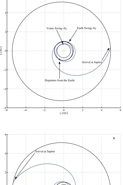
a

Earth Swing−by Venus Swing−by

Departure from the Earth

−6 −4 −2 0 2 4 6

−6 −4 −2 0 2 4 6

x [AU]

y [AU]

Earth Swing−by Venus Swing−by

Departure from the Earth

Arrival at Jupiter

b

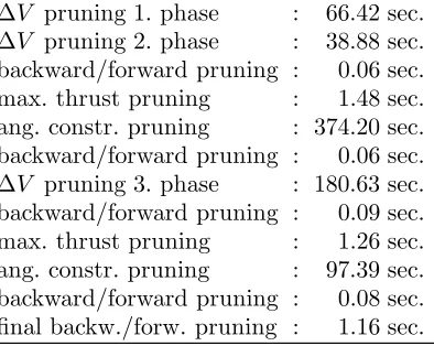
Table 3. Parameter settings for the pruning of the EVEJ sequence.

sequence

: Earth – Venus – Earth – Jupiter

launch window

: [3745

,

6840] (days after 01

.

01

.

2000)

time of flight phase 1

: [100

,

200] (days)

time of flight phase 2

: [300

,

400] (days)

time of flight phase 3

: [1000

,

2000] (days)

|

D

(

I

0

)

|

: 80

|

D

(

I

)

|

: 80

|

D

(

I

)

|

: 100

|

D

(

I

)

|

: 120

range of

k

, i

= 1

,

2

,

3

: [0

.

01

,

2]

|

D

(

I

)

|

: 20

|

D

(

I

)

|

: 20

|

D

(

I

)

|

: 20

∆

V

: 5 (

km/s

)

∆

V

2

: 5 (

km/s

)

∆

V

3

: 5 (

km/s

)

max. departure velocity : 10 (

km/s

)

max. terminal velocity

: 30 (

km/s

)

r

Venus

: 6750 (

km

)

r

Earth

: 6750 (

km

)

Table 4. Running times for sequence EVEJ (see Section 6.2).

∆

V

pruning 1. phase

:

66.42 sec.

∆

V

pruning 2. phase

:

38.88 sec.

backward/forward pruning :

0.06 sec.

max. thrust pruning

:

1.48 sec.

ang. constr. pruning

: 374.20 sec.

backward/forward pruning :

0.06 sec.

∆

V

pruning 3. phase

: 180.63 sec.

backward/forward pruning :

0.09 sec.

max. thrust pruning

:

1.26 sec.

ang. constr. pruning

:

97.39 sec.

backward/forward pruning :

0.08 sec.

final backw./forw. pruning :

1.16 sec.