An Introduction to Matlab and Mathcad

(1)

Matlab and Mathcad

Spring 2014 Edition

(2)

(3)

Many thanks to Greg Hartman for his huge amount of help with the LA_TEX layout.

Thanks to students for finding errors in the drafts leading up to this text, including Chris Fraser, Stephen States, Heather Chichura and Joey Bishop.

(4)

(5)

A Note to Students, Teachers, and other Readers

This text is used in a mathematical software course at VMI that provides an introduction to Matlab and Mathcad. However, it is also intended to be a coursebook instead of an all inclusive resource. I encourage my students to take full advantage of the built-in help capabilities of these software packages, addi-tional texts (I keep a few in a small library that is always available to students) and to use Google - I certainly did when learning the material and still do today.

This text is much shorter than a traditional text. I have tried to provide the right amount of discussion and examples. The exercise sets have a small number of problems, but I assign all of them when I teach the course. I have tried to give problems that come from real-world situations and contemporary data and aren’t simply contrived just to fill space. Some of the problems reference the electronic course management system at VMI (Angel), but these can be ignored as the data sets are also included in the Appendix.

This text is also an “open” text. If you wish to change the text for your needs, please do so. I would also share source files if you are interested. The Creative Commons copyright must be honored and that any changes be ac-knowledged and that the resulting work be used only in non-commercial areas.

Note that throughout the text, I make reference to colors (regarding text or pictures). This book is printed in black and white on purpose, but you can contact me for the full color pdf version (www.vmi.edu/math>faculty).

I welcome any comments or corrections.

Sincerely,

(6)

(7)

Thanks iii

Preface v

Table of Contents vii

1 Matlab: Introduction 1

1.1 Matlab: Introduction . . . 1

1.2 Matlab: Layout . . . 1

1.3 Matlab: Command Window Examples . . . 3

1.4 Matlab: Editor . . . 4

1.5 Matlab: Headers . . . 5

1.6 Matlab: Editor Tips . . . 6

Exercises . . . 8

2 Matlab: Matrices 9 2.1 Matlab: Matrices . . . 9

2.2 Matlab: Using Matrices . . . 12

2.3 Matlab: Matrix Operations . . . 14

2.4 Matlab: Common Matrix Functions . . . 15

2.5 Matlab: Systems of Equations . . . 19

Exercises . . . 21

3 Matlab: Functions 23 3.1 Matlab: Built-In Functions . . . 23

Exercises . . . 29

4 Matlab: Graphics 30 4.1 Matlab: Graphics . . . 30

Exercises . . . 35

5 Matlab: User Defined Functions 37 5.1 Matlab: User-Defined Functions . . . 37

(8)

6 Matlab: Input/Output 43

6.1 Matlab: Input Commands . . . 43

Exercises . . . 50

7 Matlab: Programming Structures 51 7.1 Matlab: Relational Operators . . . 51

7.2 Matlab: Logical Operators . . . 51

7.3 Matlab: ifandswitchcommands . . . 53

7.4 Matlab: forandwhileLoops . . . 54

Exercises . . . 57

8 Matlab: Applications 58 8.1 Matlab: Numerical Methods . . . 58

8.2 Matlab Traveling Salesman . . . 60

9 Matlab: Curve Fitting 63 9.1 Matlab: Curve Fitting . . . 63

Exercises . . . 68

10 Mathcad: Introduction 70 10.1 Mathcad: Introduction . . . 70

11 Mathcad: Entering Equations 72 11.1 Mathcad: Equations . . . 72

11.2 Mathcad: Editing Equations . . . 77

11.3 Mathcad: Units . . . 79

Exercises . . . 81

12 Mathcad: Given/Find and Solve 82 12.1 Mathcad: Given/Find Blocks . . . 82

12.2 Mathcad: Solve Blocks . . . 84

Exercises . . . 86

13 Mathcad: Functions 87 13.1 Mathcad: Built-in Functions . . . 87

13.2 Mathcad: User-Defined Functions . . . 88

Exercises . . . 90

14 Mathcad: Matrices 91 14.1 Mathcad: Matrix Definition . . . 91

14.2 Mathcad: Editing Matrices . . . 93

14.3 Mathcad: Referencing Parts of Matrices . . . 95

14.4 Mathcad: Solving Systems of Linear Equations . . . 97

(9)

15 Mathcad: Graphing 103 15.1 Mathcad: Graphing . . . 103 Exercises . . . 110

16 Mathcad: Curve Fitting 111

16.1 Mathcad: Curve Fitting . . . 111 Exercises . . . 116

17 Mathcad: Calculus and Symbolics 118 17.1 Mathcad: Calculus . . . 118 17.2 Mathcad: Symbolics . . . 119 Exercises . . . 121

Appendix 123

(10)

(11)

Matlab: Introduction

In this section, we discuss the basics of Matlab.

1.1

Matlab: Introduction

There are many different software packages available. It’s important to under-stand the different capabilities of each as one software package may be the best tool depending on the task. Here, we introduce Matlab, which stands for MA-Trix LABoratory. Matlab is cost-effective, easy to learn and blends powerful number crunching capabilities with graphical display. It is an excellent tool for working with large data sets.

Other packages that you may wish to consider, include Mathematica, Maple, Fortran, C, C++, or Java. In some cases, even a basic TI calculator or Excel is the appropriate tool.

Matlab has become the industry standard for use in many fields includ-ing Mathematics, Bioinformatics, Finance, and Engineerinclud-ing. The basic Matlab package includes the core package and Simulink, a platform for modeling dy-namic systems. Matlab can also be enhanced through the addition of “tool-boxes” (available from Mathworks) including such topics as Control Systems, Image Processing, Splines and SimBiology.

1.2

Matlab: Layout

(12)

You can customize how the layout appears, but there are a few main com-ponents:

Command Window

The command window is where you can perform basic calculations, enter commands, run programs, and view the numeric output.

Command History

The command history keeps a record of past commands that were entered in the command window. To run a command again from the command history, you can simply double click it. Or, if you want to alter the command before running it, you can click and drag it to the command window, change it and then run it (by hitting Enter).

Directory and Workspace (in tabs)

(13)

Current Directory

When you run any program, it is important that your Current Directory is set to the location of your program. You can also run programs in a different directory by setting the “path” to that directory. To keep it simple, we will not explain how to do this here, but refer you to the help files.

Help

The help capabilities in Matlab are well documented. It does take some time to understand Matlab syntax, but if a user is familar with another programming language, the commands are easy to pick up. Functions in Matlab are also well named, so you can often guess the name of a function that you may need.

1.3

Matlab: Command Window Examples

Let’s try some basic examples in the command window. Enter 5+5 in the com-mand window (and press Enter)

>> 5+5 ans =

10

The value 10 has been assigned to the variableans. Next, try the following

>>a=5+5 a=

10

>>b=5+5; % the semicolon suppresses output.

A few things to note. First, assignment of values to the variables is right to left (whatever is on the right of the equals sign is assigned to the variable on the left). Here, both both a and b are equal to 10, but onlya’s value is displayed because the semicolon is used to suppress the output to the screen. This is a very useful tool in programs where, for example, you want to hide the intermediate calculations.

While there are thousands of commands in Matlab, here are a few that you will use often:

clc clears the command window

clear all clears all the variables

clear variablename clears the variable namedvariablename close all closes all open plot windows

(14)

There are several rules about the naming of variables (look those up in Help or Google), but in particular, all variable names must start with a letter and all variables are case sensitive (upper case and lower case letters are considered different)!! So, for example, the variablesMathandmathare treated as different variables.

One final “peculiar” aspect of Matlab, is that you can only edit the line you are on!! You can however recall previous commands with the up and down arrow keys, or type text and use the up and down arrow keys to scroll through the commands starting with that text.

1.4

Matlab: Editor

It is tedious to type everything into the command window, not to mention trying to fix any errors. We now look at theEditor, where you will write your Matlab script files (basic programs) andfunction files (user-defined functions).

As with many aspects of Matlab, there are usually many ways to perform a task. To start the Editor window, you can either type editin the command

window or you can click on the “new script” button .

(15)

There are few more key parts to this file. Any text that follows a percent sign (%) is acommentand is colored green. These are ignored when the program is actually run, but are an important part of the documentation of the file. It is crucial that you document your files properly both to remind yourself what parts of the program do and to inform any other users that may work with the program in the future.

As you type lines into the program (hitting Enter at the end of the lines), either orange or red lines may appear on the right. You can hover your cursor over these lines to see related messages. In general, orange lines are suggestions, for example, that you should add semicolons on the end of lines to suppress output, or perhaps that another command would be better. Red lines indicate errors. You should pay close attention to these. The messages related to red lines may indicate missing parentheses, a missing “end” to close a loop, or something worse, like improper syntax. In this particular file, we are missing a semicolon in the definition of the variable a (the orange line) and haven’t completed the line for the definition ofc(the red line).

When you save this program, the file name will have a “.m” extension. We refer you to the help files for proper naming conventions of files (and variables in general).

1.5

Matlab: Headers

For each assignment for this course, you will be submitting either a script or function M-file. At the top of each file, you must include a descriptive header (as comments). They must look like the following, adjusted to fit your name, the date, etc.

% Troy Siemers

% Program Name: Assignment1.m % Date: 10 January 2010

% Course: MA110

% Description: In this assignment, we focus on how

% matrices are entered and referenced in Matlab. We also % use component-wise multiplication and

% matrix exponentiation.

(16)

1.6

Matlab: Editor Tips

Here we include some tips and keyboard shortcuts that come up often and can save time. Note that many of these are accessible by using the right mouse button while in the Editor.

Block Commenting

Instead of deleting code, it is often adventageous to simply “comment it out” for later editing. To do this, simply highlight the code that you wish to comment out and use Ctrl + R. Note that if you only want to comment out a single line, just make sure your cursor is on the line and useCtrl + R(you don’t have to highlight the whole line). You can uncomment any of these later by highlighting any comment lines and using Ctrl + T.

Running Code

There are several ways to execute your files, but there are a few short-cuts when running script files. To run the entire file, you can either use the F5key

or click on the green “run” button . To see how smaller blocks of code may run, you can highlight sections of the code and use theF9button.

Indenting

Inside of several structures, like loops, it is important that you indent the code properly. This not only for correct syntax, but also makes for easier read-ing. To make sure code is indented in the right way, simply highlight the code and typeCtrl + I.

Example 1

For this example, you could run these commands one at a time at the>>in the Command Window, but we will create a script M-file in the Editor, which we open by typingeditand hitting return or you can click on the “new script”

button . Enter the following commands on separate lines:

SideLength = sqrt(5) Value = cos(pi) DegValue = cosd(180) radius = 5;

Area = pi * radius ∧ 2

(17)

this chapter, but another easy way is to go to the Command Window and type

testat the>>line. The output for this file should look like:

SideLength = 2.2361 Value =

-1 DegValue =

-1 Area =

78.5398

(18)

Chapter 1 Exercises

1. Which of the following are valid and useable variable names? Explain your answers

a. Homework 1

b. 1Homework

c. Homework#1

d. Homework 1

e. HoMeWoRkNuMbEr1

2. Compute the following using the correct order of operations

a. 2−4∗(53−2+ 2∗(5 + 6))

b. 2− 4∗5 3−2

2∗(5 + 6)

c. 2−4∗5 3−2

2 5 + 6

3. The volume of a truncated pyramid with a square base is given by

V =1 3(a

2

+ab+b2)h

wherehis the height,ais the length of one of the sides of the base andbis the length of the sides of one of the top (also a square). Find the volume ifa= 5, b= 3, h= 10

by first defininga, b and h as separate variables and then definingV in terms of them.

4. The escape velocity from a planet is given by v =

r

2GM

R where G is the

gravitational constant,M is the mass andRis the radius of the planet. Compute the escape velocity of both earth and the moon using an online source to find the constants. In each case, first define G, M and R and then define v in terms of them. Make sure to give the citation of your source.

5. Stirling’s formula for computing the factorial is given byn! ≈√2πnn e

n . For each of n= 1,2,3,· · ·,20, compute both sides of this approximation. Hint: Use thefactorialcommand in Matlab.

6. In considering Stirling’s formula, since the numbers grow so quickly in using the factorial, it can be advantageous to use the natural logarithm function. A related approximation is given by ln(n!) ≈ nlnn−n. Compute the differenceln(n!)−

(19)

Matlab: Matrices

In this section, we discuss how matrices are created, referenced and used in calculations.

2.1

Matlab: Matrices

Each variable in Matlab is stored as a matrix, which is an array of numbers arranged in a rectangle of m rows and n columns. One says that such a matrix is an m by n matrix, written as m×n. Avectoris any matrix that has either only one row (a “row vector”) or one column (a “column vector”). A scalar, or number, is stored as a matrix that has exactly one row and one column (i.e, a 1×1 matrix).

Let’s look at some examples of how matrices are entered in Matlab. Each matrix is enclosed in the symbols [ and ], each comma (or space) separates entries on the same row and each semicolon indicates a new row.

Example 2

>> A = [1,2,3,4;5,6,7,8](orA = [1 2 3 4;5 6 7 8])

gives the 2×4 matrix

A =

1 2 3 4 5 6 7 8

and

>> B = [1; 6; 0; 9]

(20)

B = 1 6 0 9

and

>> C=[3]

gives the 1×1 matrix (i.e. a scalar)

C = 3

You may have noticed that the semicolon is used in a new way in the last example. It is perhaps unfortunate, but there are symbols that are reused throughout Matlab code (including the semicolon, colon and comma) and the meaning of a particular symbol will depend on context. Semicolons are used insidematrix definitions to indicate a new row while semicolons are used at the end of a line to suppress output. Let’s look at a few more examples.

Example 3

Suppose we wanted a matrix with the values 1 through 19 in a single (row) vector. We could enter this as

>> M = [1 2 3 4 5 6 7 8 9 10 11 12 13 14 15 16 17 18 19]

although this takes a little while to type (what if we wanted 1 to 1000?!). Instead we use thecolon operator. The syntax to create this same matrix of 1 to 19 is shortened to

>> M = [1:19].

In the last example, we can think of the colon as a “range operator.” Note that Matlab also accepts the slightly shorterM = 1:19as well, which will be useful when we come to loops. In fact, the colon is more flexible (pun intended?) as we see in the next example.

Example 4

The matrix defined as

(21)

is the same as if we typed

>> N = [1 3 5 7 9 11 13 15 17 19].

What is going on in this example? Well, the general form in using two colons this way is

start value : step size : end value

InN, the 2 means to simply count “by twos” starting at 1 and ending at 19. There’s a slight limitation in that if we tried P = [1:2:20] we would also getPto equal [1 3 5 7 9 11 13 15 17 19]. Where’s the 20? Well, the syntax ofstart:step:endactually means to begin atstart, add thestep

one at a time and then stop at the point where adding one more step size would take us past theend value. So, in the matrix P, we have to stop at 19 since adding two more would take us to 21 (past theendvalue of 20). But, suppose we actually wanted to end exactly at your last value? That’s where we use the commandlinspaceinstead.

Example 5

>> P = linspace(1,6,4)

Here we get

P =

1.0000 2.6667 4.3333 6.0000

You can see that we started at 1 and ended at 6 and have 4 total values. That’s the exact syntax:

linspace(start,end,number of values)

There are two special matrices that come up a lot too:

Example 6

>> G = ones(3,4)

gives the 3×4 matrix of all ones:

G =

(22)

>> H = zeros(2,5)

gives the 2×5 matrix of all zeros:

H =

0 0 0 0 0 0 0 0 0 0

2.2

Matlab: Using Matrices

Let’s look at how we can reference parts of a matrix.

Example 7

Consider the matrix A = [1 2 3 4;5 6 7 8]. There are actually two ways to view this matrix, either as a rectangular array of 2 rows and 4 columns, or as a list of 8 elements. Suppose we wanted to isolate the 7 in the matrix A

and store it as the variabletemp. First, we can think of the 7 as being located in the second row and third column. In this case, we can type:

>> A = [1 2 3 4;5 6 7 8]; >> temp = A(2,3)

with the result being:

temp = 7

Second, we can think of 7 as being one of the eight elements total. But, it is crucial to realize that we count elements in this way using a “column prece-dence.” This means that we count, one at a time, down the columns. This means that we can think of 7 as being located in the 6th entry, or:

>> temp = A(6)

also gives the result:

temp = 7

For completeness, in the last example, if we think ofAas a matrix:

(23)

or, thinking ofAas a vector:

A(1) = 1 A(3) = 2 A(5) = 3 A(7) = 4 A(2) = 5 A(4) = 6 A(6) = 7 A(8) = 8

If we wanted to store the entire first row ofAin the variablefirstrow, we would say that we want “all four columns of the first row.” This suggests that we can use the colon operator to shorten our work. Namely,

>> firstrow = A(1,1:4)

which gives

firstrow = 1 2 3 4

But, there’s an even shorter way to do this! If the colon doesn’t have a start and end value, it simply lists all possible values! Namely,

>> firstrow = A(1,:)

also gives

firstrow = 1 2 3 4

Ok, now what if we wanted the first row, but not the element in the first column? There are two ways to do this. First, we can use the colon as:

>> mostoffirstrow = A(1,2:4)

which gives

mostoffirstrow = 2 3 4

But, what if the matrix changes and we don’t know how big A has changed to? Those sneaky programmers at Mathworks have a work around:

>> mostoffirstrow = A(1,2:end)

also gives

(24)

2.3

Matlab: Matrix Operations

Here we will explore the algebra of matrices. It would be wise for the reader to have a basic knowledge of matrix algebra (or even linear algebra), but we will try and give plenty of explanatory examples.

Just as for scalars, many of the common algebraic operations apply to ma-trices. The symbols + and −carry over quite nicely in “element-by-element” operations as one would expect (or at least hope for). Similarly, if you want element-by-element multiplication, division, or even exponentiation, these are given by .∗, ./ and .∧ (yes, those each have a preceeding period and are pro-nounced“dot times”, “dot divide”and“dot exponent”). Operations like “regular” multiplication, division, exponents, etc. have a very different meaning than one who hasn’t been exposed to linear algebra might expect. We also have operations like the matrix transpose.

Let’s look at some examples using the matricesA = [1 2 3 4;5 6 7 8]

andB = [1; 6; 0; 9]. Again,

A =

1 2 3 4 5 6 7 8

and

B = 1 6 0 9

Example 8 Scalar Multiplication

Here we show how to multiply every entry in a matrix by a scalar:

>> A = [1 2 3 4;5 6 7 8];3*A

gives

ans =

3 6 9 12 15 18 21 24

One special operation for matrices is the matrixtranspose, given by either

transpose(A)or the shorterA'. The transpose of a matrix is another matrix with the rows and columns interchanged.

Example 9 Transpose

(25)

ans = 1 5 2 6 3 7 4 8

and

>> B = [1; 6; 0; 9];B'

ans =

1 6 0 9

The exampleA∧2 gives an error sayingAmust be square (here it is good to know some linear algebra), butA.∧2 gives element-by-element squaring:

Example 10 Element by element squaring

>> A = [1 2 3 4;5 6 7 8];A.∧2

ans =

1 4 9 16 25 36 49 64

Finally, we can create “block” matrices from smaller matrices by treating them as elements themselves and using the comma (or space) and the semicolon to create rows and columns. We just have to make sure the dimensions of the matrices line up properly. For example, we can stack two matrices.

Example 11 Stacking Matrices

>> A = [1 2 3 4;5 6 7 8];B = [1; 6; 0; 9];AoverBprime = [A ; B']

AoverBprime = 1 2 3 4 5 6 7 8 1 6 0 9

2.4

Matlab: Common Matrix Functions

size

and

length

(26)

num-ber of rows and columns inM.

Example 12 size of a matrix

>> A = [1 2 3 4;5 6 7 8];size(A)

ans = 2 4

and

>> B = [1; 6; 0; 9];size(B)

ans = 4 1

Thesize command is also what is known as an “overloaded” function in that it can be used in a couple of ways. Suppose we only wanted to know only the number of rows in a matrix M. We could find thesize(M), store this as a variable and then select the first entry. Instead, the sizecommand takes a second entry that will allow us to get what we want.

Example 13 Number of Rows or Columns Using size

>> A = [1 2 3 4;5 6 7 8];size(A,1)

ans = 2

(the number of rows)

and

>> A = [1 2 3 4;5 6 7 8];size(A,2)

ans = 4

(the number of columns).

The length of a vector (either a row or column) is simply the number of elements in the vector:

Example 14 Length of a vector

(27)

>> length(c)

ans = 5

However, the “length of a matrix” is defined in Matlab as the larger of the number of rows and the number of columns. That is,length(A)is equivalent tomax(size(A)).

max

and

min

These two functions are (almost) self explanatory. For the matrix that we are using, A = [1 2 3 4;5 6 7 8], if we try max(A), we get 5 6 7 8. What’s going on? Remember that Matlab works on column precedenceso that what max is doing is not finding the maximum value of the entire ma-trix, but instead finding the maximums of each column. The only exception occurs when the starting matrix is either a row or column vector. For exam-ple, forB = [1; 6; 0; 9],max(B)does give us9(the largest value inB). So, to get the largest element inA, we would have to “nest” the functions as

(28)

sum

and

prod

Once again, these seem reasonably named functions (see previous bullet). And once again, they return not the sum\product of every entry in matrix, but the column sums\products with the exception being for vectors, in which case you do get the sum\product of every entry in the vector. But, what if you want to get the sum along the rows? Well, once againsumis an overloaded operator and we can use:

Example 15 Column and Row sums

>> A = [1 2 3 4;5 6 7 8] >> sum(A)

ans =

6 8 10 12

(the column sums)

and

>> sum(A,2)

ans = 10 26

(the row sums)

For those that know more linear algebra, we list some familar commands.

cross

and

dot

These are the functions to find the cross product or dot product of two vec-tors usingdot(v1,v2)andcross(v1,v2). A few things to note. First, the vectors both have to be the same length, but it doesn’t matter if they are both row vectors, both column vectors, or even one of each. Second, for the cross product, recall that you need them both to be of length 3 (i.e. each of dimension 1×3 or 3×1).

det

and

inv

(29)

eye

The folks at Mathworks do have an interesting sense of humor. To create the 5×5 identity matrix, for example, you could type all 25 entries of ones and zeros, or you can use the commandeye(5). Get it? “eye”? Get it? Nevermind.

2.5

Matlab: Systems of Equations

We can use matrices to solve systems of linear equations. Here it is a good idea to read up a bit on some matrix algebra.

Suppose we have the following system of equations:

 



3x+ 2y−z = 10

−x+ 3y+ 2z = 5 x−y−z = −1

 



We will solve this system, i.e. find the values of the variables that satisfy all of the equations simultaneously, in three ways: using reduced row echelon form, using matrix inverses, and using “left division.”

Method 1: Reduced Row Echelon Form

Here we create the “augmented matrix” of the coefficients of the variables with the constants to the right of the equals signs.

>> AugmentedMatrix = [3 2 -1 10;-1 3 2 5;1 -1 -1 -1]; >> rref(AugmentedMatrix)

ans =

1 0 0 -2 0 1 0 5 0 0 1 -6

This tells us that there is only one way to solve this system, i.e. only one solution, namely x = -2, y = 5, z = -6. You can check that is correct by substituting these values back into the system of equations:

 



3(−2) + 2(5)−(−6) = 10

−(−2) + 3(5) + 2(−6) = 5 (−2)−(5)−(−6) = −1

 



(30)

Method 2: Using the matrix inverse

Here we create two matrices, one for the coefficients of the variables and one for the constants to the right of the equals signs. Note that we can define these on the same line to save space:

>> Coeffs = [3 2 -1;-1 3 2;1 -1 -1]; Constants=[10; 5; -1];

Since the determinant ofCoeffsis non-zero (check!) we can solve the sys-tem with the inverse:

>> inv(Coeffs)*Constants

ans = -2

5 -6

This also tells us that the only solution isx = -2, y = 5, z = -6.

Method 3: Using left division

The motivation for this method is complicated. We suggest that you read the Matlab documentation on left (and right) division of matrices. Again we create the two matrices,CoeffsandConstants

>> Coeffs = [3 2 -1;-1 3 2;1 -1 -1]; Constants=[10; 5; -1];

and use the backslash (be careful to use the correct slash):

>> Coeffs\Constants

ans = -2

5 -6

(31)

Chapter 2 Exercises

1. Basic calculations

a. Using colons, create the matrix that contains the numbers from 1 to 491 by steps of 10.

b. Usinglinspace, create the matrix that contains the numbers from 1 to 491 by steps of 10.

c. Using colons, create a1×50matrix containing evenly spaced numbers from 1 to 32 (inclusive).

d. Usinglinspace, create a 1×50matrix containing evenly spaced numbers from 1 to 32 (inclusive).

2. Consider the5×5“Hilbert matrix”

H5=

     

1 1/2 1/3 1/4 1/5 1/2 1/3 1/4 1/5 1/6 1/3 1/4 1/5 1/6 1/7 1/4 1/5 1/6 1/7 1/8 1/5 1/6 1/7 1/8 1/9

     

a. Find the determinant ofH5.

b. Find the transpose and inverse ofH5.

c. Using the commands in the text, find the dimensions ofH5, the column sums, and the row sums ofH5.

d. Use themaxfunction to determine the value of the maximum entry ofH5.

e. Find the eigenvalues and eigenvectors ofH5.

f. Find the matricesH2

5, H5.∧2andH5./H5 and explain your answers. g. By referencingH5, create a matrix that consists of the 2nd and 3rd rows of

H5 (do not simply retype the entries).

3. Counterclockwise rotation in two dimensions (about the origin) can be done through matrix multiplication (multiplying on the left) by the matrix

cosθ −sinθ

sinθ cosθ

Rotate the point (x, y) = (−2,3) counterclockwise about the origin by each of

θ= 30◦,90◦and200◦and give the final positions in each case.

4. Counterclockwise rotation in two dimensions about an arbitrary point, P, can be done by a translation (movingP to the origin), rotation about the origin (through matrix multiplication as in the last problem), and then retranslation (of the origin back toP) .

(32)

5. Rotation in 3-dimensions is a more difficult process. For example, if you rotate the point(1,0,0)counterclockwise around the z axis, you will arrive at the point

(0,1,0). Look up (online) for the matrix that corresponds how to rotate by an angle

θ around the z axis in 3D and make sure you cite the online source. Implement this matrix to indicate the rotation of (1,0,0) about the z axis by θ radians for

θ=π/4, π/2andπ/8.

6. In computing an approximating function for a set of data, a spline is often used. The theory of splines is covered in numerical analysis, but for a specific data set, the following system of equations must be solved.

     

    

0.28S1 + 0.1S2 =−64.65

0.1S1 + 0.34S2 + 0.07S3 =−54.81

0.07S2 + 2.16S3 + 1.01S4 =−8.43

1.01S3 + 2.58S4 + 0.28S5 =−7.92

0.28S4 + 1.42S5 =−2.78

     

    

Find the values forS1 throughS5by solving this system in three ways:

a. Using the commandrref. b. Using left division.

(33)

Matlab: Functions

In this section, we look at some functions that are built-in to Matlab. In a later section, we discuss how a user may write their own.

3.1

Matlab: Built-In Functions

(34)

In discovering what a function does, we suggest to simply try it. Let’s start with the matrixA = [1 2 49 4;25 36 3 81]and look at the output from several functions. First type in

>> A = [1 2 49 4;25 36 3 81]

• sqrt(A)

The output:

>> sqrt(A) ans =

1.0000 1.4142 7.0000 2.0000 5.0000 6.0000 1.7321 9.0000

is (hopefully) what you might expect. It finds the square root of each of the entries. If you know a little more linear algebra and was expecting the “prin-cipal” square root, or a matrix B so that B * B = A, this is created using

B = sqrtm(A).

• sin(A), sind(A)

The functionsin(A)finds the sine of every entry inA, assuming the entries ofAare in radians:

>> sin(A)

ans =

0.8415 0.9093 -0.9538 -0.7568 -0.1324 -0.9918 0.1411 -0.6299

and the function sind(A) does the same, but assumes the entries of A are in degrees:

>> sind(A)

ans =

0.0175 0.0349 0.7547 0.0698 0.4226 0.5878 0.0523 0.9877

The other trigonometric functions are similarly named.

• exp(A), log(A), log10(A)

(35)

>> exp(A)

ans = 1.0e+035 *

0.0000 0.0000 0.0000 0.0000 0.0000 0.0000 0.0000 1.5061

>> log(A)

ans =

0 0.6931 3.8918 1.3863 3.2189 3.5835 1.0986 4.3944

>> log10(A)

ans =

0 0.3010 1.6902 0.6021 1.3979 1.5563 0.4771 1.9085

We do see something curious here for the functionexp(A). It looks like all of the entries are zero until a closer look shows the leading term “1.0e+035 *”. This means that every entry in the answer is multiplied by this factor 1035 _(a rather large number). The fact that the other entries look like zero is that there aren’t enough decimal places to store each answer.

• mean(A), median(A), std(A)

These are some of the basic statistical functions. The output for these are the mean, meadian, and standard deviation of the columns ofA.

>> mean(A)

ans =

13.0000 19.0000 26.0000 42.5000

>> std(A)

ans =

16.9706 24.0416 32.5269 54.4472

>> median(A)

ans =

(36)

• sort(A), sortrows(A)

The command sortrearranges the data in the columns of Ain increasing order. The command sortrowssorts the rows ofAin increasing order (deter-mined by the first column).

>> sort(A)

ans =

1 2 3 4 25 36 49 81

>> sortrows(A)

ans =

1 2 49 4 25 36 3 81

However, both of these functions can take other arguments. For example, thesortfunction can also be used to sort the columns, or can sort using either ‘descend’ or ‘ascend’. Thesortrowsfunction can also be used to sort accord-ing to other columns. See the Help files for more details.

• flipud(A), fliplr(A)

These two functions are abbreviations of “flip up-and-down” and “flip left-to-right”. That’s exactly what they do:

>> flipud(A)

ans =

25 36 3 81 1 2 49 4

>> fliplr(A)

ans =

4 49 2 1 81 3 36 25

• find

The functionfindis used to located the position of values in a matrix.

(37)

ans = 1

A couple of comments about this example. First, there is a double equals sign in A==1. There will be more about this in a future chapter (on relational operators), but you can read this as a question “doesA equal 1?.” The entire line find(A==1)indicates the location where the (element of)Adoes in fact equal 1 (namely the first entry). Another example:

>> find(a>5)

ans = 2 4 5 8

Here we must again remember to read down the columns ofAto get to the 2nd, 4th, 5th and 8th entries. We can tweak this last example to get the exact rows and columns containing entries greater than 5:

>> [r,c]=find(A>5);[r,c]

ans = 2 1 2 2 1 3 2 4

Here we have given thefindfunction two outputs to write to, the variables

r and c, which are displayed together for easier reading using [r,c]. The output indicates that the entries ofA that are greater than 5 can be found in the 2nd row & 1st column, 2nd row & 2nd column, 1st row & 3rd column, and 2nd row & 4th column.

In the next example, we investigate the functionmeshgrid. Themeshgrid

function is used to transform vectors xand yinto arrays Xand Yof sizes ap-propriate for computation and plotting.

Example 16 Usingmeshgrid

Suppose we wanted to compute the area of a triangle for all possible combi-nations of the base, ranging from 7 to 10 units, and the height, ranging from 2 to 6 units. Here’s the set up (output suppressed):

(38)

>> Height = 2:6;

Now, we can’t just multiply these two matrices together, nor can we “dot multiply” them either, since the dimensions ofBase, 1×4, andHeight, 1×5, do not line up properly in either case. Instead we resize usingmeshgrid:

>> [NewBase,NewHeight] = meshgrid(Base,Height)

This creates two matrices,NewBaseandNewHeight, which are both 5×4. We did not suppress the output, so one can see that these are:

NewBase = 7 8 9 10 7 8 9 10 7 8 9 10 7 8 9 10 7 8 9 10

and

NewHeight = 2 2 2 2 3 3 3 3 4 4 4 4 5 5 5 5 6 6 6 6

We can now “dot multiply” them together:

>> Area= (NewBase.*NewHeight)/2

Area =

(39)

Chapter 3 Exercises

1. Consider a triangleABC. Suppose the length of the sidesAB andAC are 3 and 4, resp. Letθ denote the angle at the vertexA. Use the law of cosines to create a table with two columns: the first column containingθ in increments of 10 degrees from 0 to 180 degrees and the second column containing the length of the sideBC. First define the variables AB, AC and θ and then define BC in terms of them. What is the average length ofBC forθbetween 20 and 150 degrees?

2. Two blocks of massesm1andm2 are connected by a string over a smooth pulley as shown. Assume thatm2> m1. If the coefficient of friction isµandr=m1/m2, then the masses will move at a constant speed (m2 slides down the slope) if the

angleθ is given bycos(θ) =−µr+

p

1−r2₊_µ2

1 +µ2 .

θ

m2

m1

a. Compute the values of the angleθifm2is twice the value ofm1andµranges from 0 to 1 in increments of 0.1.

b. Compute the values of the angleθifm2 is ten times the value ofm1 andµ ranges from 0 to 1 in increments of 0.1.

c. What can you say ifm1=m2?

3. Write a file that will convert a given number of seconds into years, days, hours, min-utes and seconds. Use this file to give the conversion for 1,000seconds,1,000,000

seconds and 1,000,000,000 seconds. Some of the following commands may help

fix,floor,mod, andrem.

4. For a continuous money stream, we have the equationF =P ert whereF is final value, r is the interest rate,P is the principal, andtis time. Use themeshgrid

and theexpcommands to find possible values ofF forP ranging from10,000to

50,000(in increments of10,000) andtranging from 0 to 10 (in increments of 1). You can select the value ofr, but use a reasonable, real-world interest rate (explain how you chose your value ofr too).

5. A uniform beam is freely hinged at its endsx= 0andx=L, so that the ends are at the same level. It carries a uniformly distributed load of W per unit length and there is a tension T along thex-axis. The deflectiony of the beam a distancex

from on end is given by

y=W ·EI

T2

cosh [a(L/2−x)] cosh(a L/2) −1

+W x(L−x) 2T

wherea2 = T /EI ,E is Young’s Modulus of the beam andI is the moment of inertia of a cross-section of a beam. If the beam is10mlong, the tension is1000N, the load100N/mandEI is104, make a table ofxversusywherexranges from 0 to 10 in increments of1m. Make sure to define the variables a, W, EI, T andx

(40)

Matlab: Graphics

In this section, we discuss the graphics capabilities of Matlab.

4.1

Matlab: Graphics

The main commands that we will use in this chapter are

plot,subplot,figureandhold

and the customizations

xlim,ylim,xlabel,ylabel, andtitle.

Plots in Matlab are created by simply “connecting the dots.” This means that you have to provide the actual coordinates of the points−both thexand y coordinates. It is not enough to simply say ploty=x2_{, you must give exactly} whichxvalues you want squared.

Example 17 Basic Plot

Define:

>> x = [1:10]; y = [4 15 7 17 8 19:23];

Then to plot the corresponding coordinates, connected by line segments, use

plot(x,y)

(41)

Let’s take the last example and add some markers and labels.

Example 18 Plot with labels

>> x = [1:10]; y = [4 15 7 17 8 19:23]; >> plot(x,y,'-->b')

>> title('My plot') >> xlim([0,11]) >> ylim([0,30])

>> text(7,15,'My function')

(42)

In this last example, you can see that there is a title, the limits on the graph are now 0 to 11 (for x) and 0 to 30 (for y), and there is text on the screen, starting at the coordinate (7,15). The symbols'-->b 'indicate that the lines should be dashed, the points marked with triangles and the lines colored blue (the default color if none is provided).

If you want to plot more than one set of data in the same figure window, there are two ways to do this. You can put both in the same plotcommand or by using theholdcommand with twoplotcommands (see next example).

Example 19 Two Functions - one plotcommand

>> x1 = [1:10];y1 = [4 15 7 17 8 19:23]; >> x2 = [3:3:12];y2 = [0 5 3 10];

>> plot(x1,y1,x2,y2,'+') >> xlim([0,13]),ylim([-1,25])

The plot is now:

So, from this example we can see that if you want to use the same plot

command, you simply list the pairings, (with any details following each pair)

x1,y1,x2,y2,x3,y3,· · ·. The default colors start with blue followed by green. The symbol'+'means that the second plot is points (not lines) marked with plus signs.

Example 20 Two Functions - twoplot commands

(43)

>> x1 = [1:10];y1 = [4 15 7 17 8 19:23]; >> x2 = [3:3:12];y2 = [0 5 3 10];

>> hold on

>> plot(x1,y1) >> plot(x2,y2,'+')

>> xlim([0,13]),ylim([-1,25])

The plot is now:

In the last example, if you didn’t include the hold command, the second plot would simply overwrite the first. Also, since we didn’t specify new colors, both plots are blue (the default color of a single plot).

Here we look at thesubplotcommand as well as bar graphs and pie charts to create multiple graphs on the same figure.

Example 21 The subplotcommand

>> x = [1,2,4,5,8]; y = [x;1:5]; >> subplot(2,3,1), bar(x)

(44)

In this example, thesubploton each line does two things. First, it (invisi-bly) subdivides the figure into rows and columns and second, it indicates where the plot will be shown (counting across the rows). That is:

subplot(# rows,# columns, location)

You can see in the example that even though the plot was “broken up” into 2 rows and 3 columns in the first three subplot lines, the fourth line re-subdivides the plot into 2 rows and 1 column so that the final plot can take up the entire bottom of the plot. Using the subplots does not require the holdcommand.

(45)

Chapter 4 Exercises

For each problem, include appropriate titles and labels. Make sure to usexlimandylim

so that the plots fit well in their figure windows.

1. The double logistic curve is defined by

y= sign(x−5)· 1−exp

"

−

x−5 50

2#!

Use the command linspace to get xvalues from −100to 100 and plot y for thesexvalues. Add appropriate labels (something simple) to the axes and a title.

2. For the functionsy=ex/5_,_y_{= sin(}_x₎_,_y₌√_x_for_x_{between 0 and 10:}

a. Plot all three on the same plot, but with different colors (uselinspacewith enough points so that the curves look smooth). Put in a descriptive title and add text inside the window to label the individual graphs.

b. Plot all three in the same figure window, but with each in their own subplot and each with its own descriptive title.

3. Plot the following curves, either on separate plot windows or as subplots in the same figure window, by first defining the parametert=linspace(0,6π)and then definingxandyin terms oft. Use the standardplotcommand to plot them and add appropriate titles. For each, adjusttfor a smoother curve as necessary.

a. Cardioid: x= 2 cost−cos 2t, y= 2 sint−sin 2t. b. Astroid: x= cos3t, y= sin3t.

c. Hypotrochoid:x= 2 cost+ 5 cos 2 3t

, y= 2 sint−5 sin 2 3t

.

d. Epicycloid: x= 6.5 cos(t)−cos(6.5t), y= 6.5 sin(t)−sin(6.5t)

4. In the same figure window, ploty = sin(t+φ) for each ofφ= 0, π/4and π/2, on the range fortfrom0to2π. Using the textcommand, label the plots inside the figure window. Also, use xlim,ylim to make the plots fit nicely in the plot window.

(46)

5. The following data are coordinates of an analemma. Look up the definition of an analemma and give a short description here. Make sure to cite your source.

y x 89.814 −4.67 83.222 −6.824 71.282 −7.7697 60.581 −7.33 50.572 −6.22 41.748 −4.759

38.36 −4.105 32.748 −3.045 26.664 −1.957 21.141 −1.146 17.445 −0.946 14.548 −1.193 13.38 −1.713 13.1497 −1.946 13.569 −2.388 14.942 −2.854 18.269 −3.087 22.189 −2.84 28.455 −1.992 34.742 −0.834 38.876 −0.117 43.349 0.607 52.124 1.824 64.591 2.842 74.997 2.775 85.45 1.196 90.649 −1.265 91.403 −2.559

As you can see, the data was unfortunately entered backwards so that the second column gives thex coordinate and the first column gives they coordinate. First enter the data into a 2-column matrix (in a variable of your choice). Usefliplr

to redefine the columns and define the variable xby referencing the first column andy by referencing the second column. Plot the data with an appropriate title. Note that you may have to adjust the data so that the analemma is a closed figure.

(47)

Matlab: User Defined

Functions

In this section, we discuss how to create new functions in Matlab.

5.1

Matlab: User-Defined Functions

Up to now, the M-files that you have created are called “script” files. Now we use the editor to create function M-files. Why would you want to do this? Well, Matlab has many built-in functions, but you may need to create your own to solve a specialized problem.

Lets look at how a function is put together. In the command window, if you were to type

>> help sin

you would get

SIN Sine of argument in radians.

SIN(X) is the sine of the elements of X.

Chapter 5 Exercises

When you submit this assignment, there should be seven separate files. Problems 1-6 should be in their own function m-files (properly commented of course). Problem 7 should be a separate script m-file that uses the code from the first 6 problems. Make sure each of your files starts with your VMI id (mine would besiemerstjFunction).

1. The height of a projectile is given by

f(t) =−9.8

2 t

2

+ 147t+ 500, t >0

Create the function ProjMotion that has one input, time, and two outputs

heightandvelocity.

2. Create an appropriately named conversion function that has one input (dollars) and one output (ConversionTable). The conversion table should contain four columns, with dollars in the first column and the conversions into Yen, Euros, and British Pounds in the next three columns (look up the current conversion rates online and cite your source).

3. Create a function called plotlines with two inputs and no outputs with the following details. The first input should be a 1×2matrix (representing the base point, B, in the plane). The second input should be a 2×2 matrix (representing two more points in the plane, P and Q). When the function is run, there should be a plot of two line segments, BP and BQ, with the two distances displayed halfway along each line.

4. Create a function calledRemRowwith two inputsMandn. The output should be a matrixNewMthat comes from removing the nth row ofM.

5. Create a function calledRemColwith two inputsMandn. The output should be a matrixNewMthat comes from removing the nth column ofM.

6. Create a function that will convert a given number of seconds (the input of the function) into years, days, hours, minutes and seconds (listed in one 1×5 matrix output). Some of the following commands may help: fix,floor,mod, andrem.

7. In this problem, you will use your functions from the previous problems, running them with specific numeric input(s).

(a) Run yourProjMotionfunction for 0 to 30 seconds in increments of 0.5 sec-onds and use the output to plottimeversusheight. Use the output of the function (and appropriate Matlab functions) to figure out at what time the object starts to fall back to the ground.

(b) Run your currency conversion function to give the output from an input

dollars) ranging from 0 to 100 in increments of 5.

(52)

(d) Run your RemRowfunction with inputs[1 2 3; 4 5 6; 7 8 9]and2. The output should be the matrix with the 2nd row removed.

(e) Run your RemColfunction with inputs[1 2 3; 4 5 6; 7 8 9]and2. The output should be the matrix with the 2nd columns removed.

(f) Run your time conversion function to give the conversion for1,000 seconds,

(53)

Matlab: Input/Output

In this section, we discuss the input/output (I/O) capabilities in Matlab.

6.1

Matlab: Input Commands

In order to run either script M-files or function M-files, the user needs to pro-vide data, either numerical or text (“strings”). The first command we consider is simply calledinput.

Example 24 Using theinput command

Here is a simple section of code to collect a person’s first name and their age.

>> FirstName = input('Enter your first name : ','s');

>> Age = input('Enter your age : ');

Once executed, the user enters values for each, say

Enter your first name : Bob Enter your age : 25

In this example, the 's' in the first input indicates that the program expects text input and the second input (without the 's') indicates that the program expects numeric input. When executed, the lines collect input one at a time. Note the textWaiting for input on the bottom left of the Matlab window while the user enters the name,Bob, and age,25. Due to the semicolons, there is no output to the screen, but the values have been stored in the variablesFirstNameandAge(see the Workspace window to confirm).

So how do we display this information? There are several ways to output this information. Here we consider the two commandsdisp(for “display”) and

(54)

We can present this information as follows.

Example 25 Using thedisp command

Using the data from the last example:

>> disp('Your first name is ') >> disp(FirstName)

>> disp('Your age is ') >> disp(Age)

which has the output:

Your first name is Bob

Your age is 25

This example is ok, but it would be nicer if the data was in one line. That’s where the command fprintfcomes in. Even though it is a formatted print “to file” you can have the output sent to the Command Window instead.

Example 26 Using the command fprintf

>> fprintf('%s is %.0f years old.\n ',FirstName,Age)

produces

Bob is 25 years old.

Certainly, there is more involved in the functionfprintf in order to pro-duce the output we want. Let’s look at the individual pieces of this example.

• The%signs are NOT for comments this time (note: they aren’t green), they are now used as place holders for the data.

• The%sindicates that a string is expected as input.

•The%.0findicates that we expect a numeric input, want zero decimal points and the value should be in Fixed-point format.

For more information on specific formats and “conversion characters” (which is what fandsare here), look at thefprintfcommand in the help files.

(55)

•The dataFirstNameandAgeare listed after this, separated by commas.

• When the command is run, Matlab places the first data value, FirstName

(i.e. Bob), in the%sposition and the second data value, Age(i.e. 25), in the %.0fposition. Got it?

Just for completeness, we can also force the disp command to act like

fprintfas follows:

Example 27 dispusing concatenated strings

>> disp([FirstName,' is ', num2str(Age),' years old.'])

produces

Bob is 25 years old.

Basically, we are displaying a string array made up of several strings through concatenation. We also see the commandnum2strwhich does exactly what it says, it converts a number into a string. This is necessary since numeric data and strings don’t play well together in Matlab. In order to create a string array, all of the parts must be strings. If we tried to run this without the num2str

command, we would get

>> disp([FirstName,' is ', Age,' years old.'])

with output

Bob is years old.

where the square indicates that the ASCII code for the value 25 is unprint-able (look it up or don’t worry about it - just remember thenum2str).

Let’s look at how to read and write larger data files next.

Example 28

(56)

2005 2006 2007 2008 2009 2010 91377 95037 107789 112870 86476 113375 84980 91183 101465 107465 86610 107119 93198 102183 112988 119934 92144 122196 93381 101604 110241 117023 89644 120497 95290 105501 112933 121062 96177 124567 92095 104636 112159 118851 100661 118346 90205 104350 110377 116770 104701 114365 91536 102630 109024 112726 108351 113141 93144 103676 111956 107723 110773 112340 98534 106913 114703 99202 114765 117377 94340 104817 109936 86513 108596 114637 95368 105306 111506 81704 107792 116157

We will now read in this data usingxlsread, plot it, and access data from it using the mouse and the graphical input commandginput(“gee-input”).

>> Steel = xlsread('WorldSteelProduction.xls');

Next, we plot the data

>> plot(1:12,Steel(2:end,:))

>> legend('2005','2006','2007','2008','2009','2010', ... 'Location','best')

The initial problem is to find the first time in 2009 that steel production is at 100,000 thousand metric tons. We use theginputcommand for the user to collect this data.

>> disp('Select the 2009 time when production is 100,000.'); >> [t,l] = ginput(1) % mouse click

(57)

A left-click creates the output to appear in the Command Window:

t =

5.8756 l =

9.9934e+004

Note that the level is listed in engineering format. If we want to finish this example with a formatted output, we could use the following:

>> fprintf('Level %6.1f occurs %3.1f months into 2009.\n',l,t)

Level 99934.2 occurs 5.9 months into 2009.

which is in mid-June 2009. Note that the accuracy of the level and time are dependent on the user’s mouse click so the output may not look exactly the same.

(58)

Key Idea 2 fprintf with matrices

If there are not enough place holders,fprintfwill cy-cle through the values in the given data matrix, USING COLUMN PRECEDENCE, until all of the values are exhausted.

Example 29

Here we use fprintfand Key Idea 2 to display a matrix of values. Find the sine, cosine and tangent of theta from 0 to 2πby steps of π/10.

>> theta=[0:pi/10:2*pi];

>> values=[theta;sin(theta);cos(theta);tan(theta)];

To display these, we can use a simple fprintf.

>> disp('Theta Sine Cosine Tangent ');

>> fprintf('%5.2f %6.2f %7.2f %9.2f\ n ',values)

gives output:

Theta Sine Cosine Tangent 0.00 0.00 1.00 0.00 0.31 0.31 0.95 0.32 0.63 0.59 0.81 0.73 0.94 0.81 0.59 1.38 1.26 0.95 0.31 3.08

1.57 1.00 0.00 16331239353195370.00 1.88 0.95 -0.31 -3.08

2.20 0.81 -0.59 -1.38 2.51 0.59 -0.81 -0.73 2.83 0.31 -0.95 -0.32 3.14 0.00 -1.00 -0.00 3.46 -0.31 -0.95 0.32 3.77 -0.59 -0.81 0.73 4.08 -0.81 -0.59 1.38 4.40 -0.95 -0.31 3.08

4.71 -1.00 -0.00 5443746451065123.00 5.03 -0.95 0.31 -3.08

(59)

(60)

Chapter 6 Exercises

When you submit this assignment, there should be three separate files. Problems 1 and 2 should be in their own function m-files (properly commented of course). Problems 3-6 should be a separate script m-file that uses the code from the first 2 problems and Excel spreadsheets on Angel. As usual, make sure each of your file names start with your VMI id.

1. For this problem, you will modify your projectile motion function from the last homework. Now, as part of your new function, ProjMotion2, plot the height

versustime, use ginput for the user to identify the maximum height, and use

fprintfto display a sentence describing the maximum height and corresponding time.

2. For this problem, modify your conversion function from the previous homework and rename it Conversion2. Now, use fprintf in order to create a nice-looking table showing conversions between Dollar, Euro, Yen, and British Pounds. Include a header for each column.

3. Run your ProjMotion2 function for time 0 to 30 seconds (in increments of 0.5 seconds) and your function Conversion2 for dollars from 0 to 100 in increments of 5.

4. Data on the Federal GDP and Deficit (as a percentage of GDP) is in a file called

GDPAndDeficitByYear.xlsx(in the Appendix in Table 1 and saved on Angel). First save this file to a directory on your computer and then use the command

xlsreadto load this file. Assign the data in the file to a variable of your choice and create a plot of year (1st column) versus GDP (2nd column, in billions of dollars) including appropriate titles and labels on the axes. Use ginput for the user to click on the first time the GDP exceeds $10 trillion. Use fprintf to display the information in a useful way.

5. Consider the data from the previous problem (loaded withxlsread from the file calledGDPAndDeficitByYear.xlsx). Now create a plot of year versus Deficit (3rd column), which is listed as a percentage of the GDP for the corresponding year. Including appropriate titles and labels on the axes. Useginputfor the user to click onallof the times the Deficit percentage has hit 10 percent and then use

fprintfto display the information in a useful way.

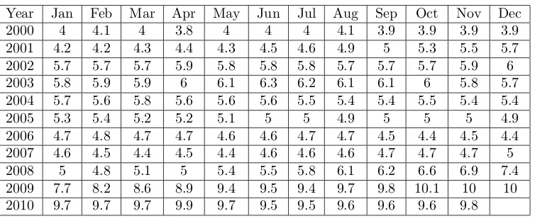
6. Data on unemployment percentages (per month) during 2000-2010 is in a file called

UnemploymentByYear.xlsx(in the Appendix in Table 2 and saved on Angel). First save this file to a directory on your computer and then use the command

(61)

Matlab: Programming

Structures

In this section, we discuss relational operators, logical operators and loop struc-tures in Matlab.

7.1

Matlab: Relational Operators

If we want to compare two values, we have the following relation operations:

< , <= , >, >=, ==, ∼=

It is helpful to read any statement involving these symbols as a question as the answer is either0(false) or1(true).

Example 30 Basic Relations

>> 3 == 4 (“is 3 equal to 4?”) gives0(false)

>> 3 <= 4 (“is 3 less than or equal to 4?”) gives1(true)

7.2

Matlab: Logical Operators

(62)

questions!

& (“and” returns true if both parts are true)

∼ (“not” returns true if the initial value is false)

| (‘or” returns true if either part is true)

xor (“exclusive or” returns true if either part is true, but NOT both true)

Example 31 Basic Logic

>> (3 >= 2) & (3+4 == 6)

ans= 0

Here, the question “is 3 greater than or equal to 2 AND 3 plus 4 equal to 6?” is answered as false (or a zero) since even though 3 is greater than 2, it is not true that 3 plus 4 is 6.

Note that there are also the operators && and || which also mean “and” and “or” but are called “short-circuited” operators (look it up). As you work with these in the Editor, orange lines on the right side of the screen may appear suggesting you use && in place of & (or vice-versa) and ||in place of| (or vice versa). Just take those suggestions and you’ll be fine.

These operations extend to matrices with an entry-by-entry comparison of matrices of the same size.

Example 32

>> a=[0,1;1,2], b=[0,0;1,1]

a = 0 1 1 2 b =

0 0 1 1

with

>> a&b, a|b, xor(a,b)

returns

(63)

ans = 0 1 1 1

ans = 0 1 0 0

One minor point to note is that while Matlab treats 0 as false, any other positive whole number is considered as true. So, in this example, even though the (2,2) entry ofais a 2, it is considered as “true” for logical comparison.

7.3

Matlab:

if

and

switch

commands

We discuss the constructs if\elseif\elseandswitch\case\otherwise

in this section.

Suppose we want to have part of our program run only under certain condi-tions. For this, we use anif\elsestructure. The basic format of this structure is:

if (put condition(s) here)

(put calculations here to be run if the conditions are met)

elseif (other condition(s))

(calculations that will run under the new conditions)

... (more elseif statements, if desired)

else

(calculations run if none of the previous conditions are met)

end

Example 33 Usingif

Let’s write a script M-file that lets a user input a number and then displays if that number is less than 5, between 5 and 10 (inclusive), or greater than 10.

number = input('Input a number ');

if number < 5

disp('Your number is less than 5.')

elseif number >=5 && number <= 10

disp('Your number is between 5 and 10.')

else

disp('Your number is greater than 10.')

end

(64)

Theswitch\casestructure is similar to the ifstructure, but has a few advantages. First of all it is easier to read and second, it is better if you are comparing strings (of possibly different lengths). The basic format is:

switch (expression to test)

case (case condition) (output in that case)

...(more cases)

otherwise

(do this if no cases are met)

end

Example 34 Using switch

Let’s check to see if a cadet is in his\her first two years at VMI.

Year = 'second class';

switch Year

case {'fourth class','third class'}

disp('You are in the first two years.')

case {'second class','first class'}

disp('You are in the last two years.')

otherwise

disp('You must be a 5th year.')

end

The cases are grouped by curly brackets so that a case will be satisfied if the value ofYearis any of the values in a specific case. Once this code is executed, theswitchcommand will look at the value ofYearand the output should be

You are in the last two years.

7.4

Matlab:

for

and

while

Loops

We discuss theforandwhileloops in this section.

Suppose we want to have part of our program re-run a preset number of times. For this, we use a forloop. The basic format of this structure is:

for (put counter conditions here) (put calculations here)

(65)

Example 35 Comparingfor and sum

Let’s compare two methods for adding up the first five integers. Using the

sumcommand we can use

>> sum(1:5) ans =

15

Now, using aforloop to create a cumulative sum:

totalsum=0; % initialize

for i=1:5

totalsum=totalsum+i;

end

disp(totalsum)

The variabletotalsumwill have value 15.

In example 35, the for loop was the long way of doing the problem (and therefore stresses the power of the sum function), but the following example shows a more in-depthforloop.

Example 36 Usingfor

Let’s find the first 10 Fibonacci numbers using the recursive definition.

%initialize the matrix

A=zeros(1,10); A(1)=0;

A(2)=1;

for i=3:10

A(i)=A(i-1)+A(i-2);

end

disp(A)

The output for this would be

A =

0 1 1 2 3 5 8 13 21 34

(66)

is met, even though we may not know how many times the loop will need to run until that happens. For this, we use awhileloop.

The basic format of this structure is:

while (put conditions for the loop to keep running)

(put calculations here)

end

Let’s rewrite the last example with a slight twist. Let’s find the Fibonacci numbers until they exceed 1000.

Example 37 Using while

%initialize the matrix (we dont know how big it will be so % we will grow it in the while loop).

A(1)=0; A(2)=1;

j=2; %initialize a counter

while A(j) < 1000

j=j+1; %move the counter along

A(j)=A(j-1)+A(j-2);

end

disp(A)

The output for this would be

A =

0 1 1 2 3 5 8 13 21 34 55 89 144 233 377 610 987 1597

(67)

Chapter 7 Exercises

When you submit this assignment, there should be five separate files. Problems 1-3 should be in one script m-file. Problems 4a and 4b should be in their own function m-files (properly commented of course). Make sure each of your files starts with your VMI id.

1. In some computer programs, a loop is necessary to add a list of numbers. Consider the cubes of the first 100 integers,13,23,33,· · ·,1003.

a. Create a matrix of the numbers 1 to 100 and use thesumcommand to find the sum of the cubes of the numbers.

b. Use aforloop to find the same sum by adding the cubes of the numbers one at a time (onto a cumulative sum).

c. A formula that you may have seen is that the sum of the cubes of the numbers

from 1 to nis given by n

2₍_n_{+ 1)}2

4 . Confirm your sum in the previous parts

using this formula.

2. Use the data in chapter 4 exercises and a loop structure to find the length of the Analemma.

3. In this exercise, you will be comparing the capabilities of the if\else and switch\case structures by creating two programs. In each program, prompt the user to enter the last name of one of the last 10 presidents of the United States. Your program should display an informative sentence in response (including the presidency number and when he served), or display an error message if the entered name is invalid. In the first program, use an if\else structure and in the second program, use a switch\case structure. Note: you will need to know how to compare strings (look in the help files).

4. Modify yourRemoveRowFunction from the previous homework in two ways (you should have two functions, perhaps calledRemoveRowIfandRemoveRowWhile)

a. In the first function, use anifstatement to have an error message displayed if the user enters an invalid row. Then prompt them to enter a new row number. In your prompt, you must indicate the allowable range of rows. Here they only have one chance to re-enter the row.

(68)

Matlab: Applications

In this chapter, we put several aspects of programming together. You will learn about the numerical methods of Riemann sums, the Trapezoidal Rule and Simpson’s rule. We’ll also investigate aspects of the Traveling Salesman problem.

8.1

Matlab: Numerical Methods

In Calculus, you learn how to use Rieman