Notes on Diffy Qs: Differential Equations for Engineers

(1)

Notes on Diffy Qs

Differential Equations for Engineers

by Jiˇrí Lebl

(2)

Typeset in LA_TEX.

Copyright c2008–2019 Jiˇrí Lebl

This work is dual licensed under the Creative Commons Attribution-Noncommercial-Share Alike 4.0 International License and the Creative Commons Attribution-Share Alike 4.0 International License. To view a copy of these licenses, visit https://creativecommons.org/licenses/ by-nc-sa/4.0/orhttps://creativecommons.org/licenses/by-sa/4.0/or send a letter to Creative Commons PO Box 1866, Mountain View, CA 94042, USA.

You can use, print, duplicate, share this book as much as you want. You can base your own notes on it and reuse parts if you keep the license the same. You can assume the license is either the CC-BY-NC-SA or CC-BY-SA, whichever is compatible with what you wish to do, your derivative works must use at least one of the licenses. Derivative works must be prominently marked as such. During the writing of these notes, the author was in part supported by NSF grant DMS-0900885 and DMS-1362337.

The date is the main identifier of version. The major version/edition number is raised only if there have been substantial changes. Edition number started at 5, that is, version 5.0, as it was not kept track of before.

Seehttps://www.jirka.org/diffyqs/for more information (including contact information). The LA_{TEX source for the book is available for possible modification and customization at github:}

(3)

Introduction

0.1

Notes about these notes

This book originated from my class notes for Math 286 at the University of Illinois at Urbana-Champaignin Fall 2008 and Spring 2009. It is a first course on differential equations for engineers. Using this book, I also taught Math 285 at UIUC, Math 20D at UCSD, and Math 4233 at OSU. Normally these courses are taught with Edwards and Penney,Differential Equations and Boundary Value Problems: Computing and Modeling[EP], or Boyce and DiPrima’sElementary Differential Equations and Boundary Value Problems[BD], and this book aims to be more or less a drop-in replacement. Other books I used as sources of information and inspiration are E.L. Ince’s classic (and inexpensive) Ordinary Differential Equations [I], Stanley Farlow’s Differential Equations and Their Applications[F], now available from Dover, Berg and McGregor’sElementary Partial Differential Equations[BM], and William Trench’s free bookElementary Differential Equations with Boundary Value Problems[T]. See the Further Readingchapter at the end of the book.

The organization of this book to some degree requires chapters be done in order. Later chapters can be dropped. The dependence of the material covered is roughly:

Introduction Chapter 1 Chapter 2

Chapter 3 Chapter 6 Chapter 7 Chapter 8 Chapter 4

Chapter 5

There are some references in chapters 4and 5to material from chapter 3(some linear algebra), but these references are not absolutely essential and can be skimmed over, so chapter 3can safely be dropped, while still covering chapters 4and 5. The textbook was originally made for two types of courses. Either at 4 hours a week for a semester (Math 286 at UIUC):

(6)

Introduction, chapter 1, chapter 2, chapter 3, chapter 4(w/o § 4.10), chapter 5(or 6or 7or 8). For a shorter version (3 hours a week) of the above course, skip chapters 4and 5. The second type of the course at 3 hours a week (Math 285 at UIUC) was:

Introduction, chapter 1, chapter 2, chapter 4(w/o § 4.10), (and maybe chapter 5, 6, or 7).

The complete book can be covered at a reasonably fast pace at approximately 75 lectures, not accounting for exams, review, or time spent in computer lab. A two quarter course can be easily run with the material, and if one does not rush, a two semester course. For example:

Semester 1: Introduction, chapter 1, chapter 2, chapter 6, chapter 7, (and perhaps bits of 4). Semester 2: Chapter 3, chapter 8, chapter 4, chapter 5.

The chapter on Laplace transform (chapter 6), the chapter on Sturm-Liouville (chapter 5), the chapter on power series (chapter 7), and the chapter on nonlinear systems (chapter 8), are more or less interchangeable time-wise. If chapter 8is covered it may be best to place it right after chapter 3. If time is short, the first two sections of chapter 7make a reasonable self-contained unit.

I taught the UIUC courses using the IODE software (https://faculty.math.illinois. edu/iode/). IODE is a free software package that works with Matlab (proprietary) or Octave (free software). The graphs in the book were made with the Genius software (seehttps://www.jirka. org/genius.html). I used Genius in class to show these (and other) graphs.

This book is available fromhttps://www.jirka.org/diffyqs/. Check there for any possi-ble updates or errata. The LA_{TEX source is also available for possible modification and customization}

at github (https://github.com/jirilebl/diffyqs).

(7)

0.2. INTRODUCTION TO DIFFERENTIAL EQUATIONS 7

0.2

Introduction to di

ff

erential equations

Note: more than 1 lecture, §1.1 in [EP], chapter 1 in [BD]

0.2.1

Di

ff

erential equations

The laws of physics are generally written down as differential equations. Therefore, all of science and engineering use differential equations to some degree. Understanding differential equations is essential to understanding almost anything you will study in your science and engineering classes. You can think of mathematics as the language of science, and differential equations are one of the most important parts of this language as far as science and engineering are concerned. As an analogy, suppose all your classes from now on were given in Swahili. It would be important to first learn Swahili, or you would have a very tough time getting a good grade in your classes.

You saw many differential equations already without perhaps knowing about it. And you even solved simple differential equations when you took calculus. Let us see an example you may not have seen:

dx

dt +x=2 cost. (1)

Here xis thedependent variableandtis theindependent variable. Equation (1) is a basic example of adifferential equation. In fact, it is an example of afirst order differential equation, since it involves only the first derivative of the dependent variable. This equation arises from Newton’s law of cooling where the ambient temperature oscillates with time.

0.2.2

Solutions of di

ff

erential equations

Solving the differential equation means findingxin terms oft. That is, we want to find a function oft, which we will callx, such that when we plug x,t, and dx_dt into (1), the equation holds. It is the same idea as it would be for a normal (algebraic) equation of justxandt. We claim that

x= x(t)= cost+sint

is asolution. How do we check? We simply plugxinto equation (1)! First we need to compute dx_dt. We find that dx_dt =−sint+cost. Now let us compute the left hand side of (1).

dx

dt +x=(−sint+cost)+(cost+sint)= 2 cost.

Yay! We got precisely the right hand side. But there is more! We claimx=cost+sint+e−t is also a solution. Let us try,

dx

dt =−sint+cost−e

(8)

Again plugging into the left hand side of (1) dx

dt + x=(−sint+cost−e

−t

)+(cost+sint+e−t)=2 cost. And it works yet again!

So there can be many different solutions. In fact, for this equation all solutions can be written in the form

x=cost+sint+Ce−t

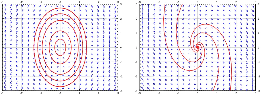
for some constantC. See Figure 1for the graph of a few of these solutions. We will see how we find these solutions a few lectures from now.

It turns out that solving differential equations

0 1 2 3 4 5

-1 0 1 2 3

Figure 1: Few solutions ofdx_dt +x=2 cost.

can be quite hard. There is no general method that solves every differential equation. We will generally focus on how to get exact formulas for solutions of certain differential equations, but we will also spend a little bit of time on getting ap-proximate solutions.

For most of the course we will look at ordi-nary differential equationsor ODEs, by which we mean that there is only one independent variable and derivatives are only with respect to this one variable. If there are several independent vari-ables, we will getpartial differential equationsor PDEs. We will briefly see these near the end of the course.

Even for ODEs, which are very well under-stood, it is not a simple question of turning a crank to get answers. It is important to know when it is easy to find solutions and how to do so. Although in real applications you will leave much of the actual calculations to computers, you need to understand what they are doing. It is often necessary to simplify or transform your equations into something that a computer can understand and solve. You may need to make certain assumptions and changes in your model to achieve this.

To be a successful engineer or scientist, you will be required to solve problems in your job that you never saw before. It is important to learn problem solving techniques, so that you may apply those techniques to new problems. A common mistake is to expect to learn some prescription for solving all the problems you will encounter in your later career. This course is no exception.

0.2.3

Di

ff

erential equations in practice

(9)

0.2. INTRODUCTION TO DIFFERENTIAL EQUATIONS 9 mathematical model. That is, we translate the real world situation into a set of differential equations. Then we apply mathematics to get some sort of amathematical solution. There is still something left to do. We have to interpret the results. We have to figure out what the mathematical solution says about the real world problem we started with.

Learning how to formulate the mathematical

Mathematical

Real world problem

interpret Mathematical

solution abstract

model

solve model and how to interpret the results is what

your physics and engineering classes do. In this course we will focus mostly on the mathematical analysis. Sometimes we will work with simple real world examples, so that we have some intuition and motivation about what we are doing.

Let us look at an example of this process. One of the most basic differential equations is the standardexponential growth model. LetPdenote the population of some bacteria on a Petri dish. We assume that there is enough food and enough space. Then the rate of growth of bacteria is proportional to the population—a large population grows quicker. Lettdenote time (say in seconds) andPthe population. Our model is

dP dt = kP, for some positive constantk>0.

Example 0.2.1: Suppose there are 100 bacteria at time 0 and 200 bacteria 10 seconds later. How many bacteria will there be 1 minute from time 0 (in 60 seconds)?

First we have to solve the equation. We claim that a solution is given by P(t)=Cekt,

whereCis a constant. Let us try:

dP

dt =Cke

kt₌

kP.

And it really is a solution.

OK, so what now? We do not knowC and we do not know k. But we know something. We knowP(0) =100, and we also knowP(10) = 200. Let us plug these conditions in and see what happens.

100= P(0)=Cek0 =C, 200= P(10)=100ek10. Therefore, 2=e10k or ln 2₁₀ = k≈0.069. So we know that

P(t)=100e(ln 2)t/10 ≈100e0.069t.

(10)

Let us talk about the interpretation of the results. Does our solution mean that there must be exactly 6400 bacteria on the plate at 60s? No! We made assumptions that might not be true exactly, just approximately. If our assumptions are reasonable, then there will be approximately 6400 bacteria. Also, in real lifePis a discrete quantity, not a real number. However, our model has no problem saying that for example at 61 seconds,P(61)≈6859.35.

Normally, the k in P0 = kP is known, and

0 10 20 30 40 50 60

0 1000 2000 3000 4000 5000 6000

Figure 2: Bacteria growth in the first 60 seconds. we want to solve the equation for differentinitial

conditions. What does that mean? Take k = 1 for simplicity. Now suppose we want to solve the equation dP_dt =Psubject toP(0) =1000 (the initial condition). Then the solution turns out to be (exercise)

P(t)= 1000et.

We call P(t) = Cet _{the general solution, as}

every solution of the equation can be written in this form for some constantC. You will need an initial condition to find out what C is, in order to find theparticular solutionwe are looking for.

Generally, when we say “particular solution,” we just mean some solution.

Let us get to what we will call the four fundamental equations. These equations appear very often and it is useful to just memorize what their solutions are. These solutions are reasonably easy to guess by recalling properties of exponentials, sines, and cosines. They are also simple to check, which is something that you should always do. There is no need to wonder if you remembered the solution correctly.

First such equation is,

dy dx =ky,

for some constantk > 0. Hereyis the dependent and x the independent variable. The general solution for this equation is

y(x)=Cekx.

We saw above that this function is a solution, although we used different variable names. Next,

dy

dx = −ky,

(11)

0.2. INTRODUCTION TO DIFFERENTIAL EQUATIONS 11

Exercise0.2.1: Check that the y given is really a solution to the equation.

Next, take thesecond order differential equation d2y dx2 = −k

2

y,

for some constantk> 0. The general solution for this equation is y(x)=C1cos(kx)+C2sin(kx).

Note that because we have a second order differential equation, we have two constants in our general solution.

Exercise0.2.2: Check that the y given is really a solution to the equation.

And finally, take the second order differential equation d2_y

dx2 =k

2

y,

for some constantk> 0. The general solution for this equation is y(x)=C1ekx+C2e−kx,

or

y(x)= D1cosh(kx)+D2sinh(kx).

For those that do not know, cosh and sinh are defined by coshx= e

x+_e−x

2 , sinhx= e

x₋

e−x 2 .

These functions are sometimes easier to work with than exponentials. They have some nice familiar properties such as cosh 0 = 1, sinh 0 = 0, and _dxd coshx = sinhx (no that is not a typo) and

d

dxsinhx=coshx.

Exercise0.2.3: Check that both forms of the y given are really solutions to the equation.

An interesting note about cosh: The graph of cosh is the exact shape a hanging chain will make. This shape is called acatenary. Contrary to popular belief this is not a parabola. If you invert the graph of cosh it is also the ideal arch for supporting its own weight. For example, the gateway arch in Saint Louis is an inverted graph of cosh—if it were just a parabola it might fall down. The formula used in the design is inscribed inside the arch:

(12)

0.2.4

Exercises

Exercise0.2.4: Show that x=e4t _{is a solution to x}000₋_12x00+_48x0₋_64x= _0.

Exercise0.2.5: Show that x=et is not a solution to x000−12x00+48x0−64x=0.

Exercise0.2.6: Is y =sint a solution tody_dt2 =1−y2? Justify.

Exercise0.2.7: Let y00+2y0−8y=0. Now try a solution of the form y =erx_{for some (unknown)}

constant r. Is this a solution for some r? If so, find all such r.

Exercise 0.2.8: Verify that x = Ce−2t _{is a solution to x}0 = _{−2x. Find C to solve for the initial}

condition x(0)=100.

Exercise0.2.9: Verify that x=C1e−t +C2e2t is a solution to x00− x0−2x=0. Find C1 and C2to

solve for the initial conditions x(0)= 10and x0₍₀₎= _0.

Exercise0.2.10: Find a solution to(x0)2+x2 =4using your knowledge of derivatives of functions that you know from basic calculus.

Exercise0.2.11: Solve:

a) dA

dt =−10A, A(0)=5 b)

dH

dx =3H, H(0)= 1 c) d

2_y

dx2 =4y, y(0)=0, y

0₍₀₎= ₁ _d) d

2_x

dy2 =−9x, x(0)= 1, x

0₍₀₎=₀

Exercise0.2.12: Is there a solution to y0 = _{y, such that y(0)}=_y(1)?

Note: Exercises with numbers 101 and higher have solutions in the back of the book.

Exercise0.2.101: Show that x=e−2t _{is a solution to x}00+_4x0+_4x= _0.

Exercise0.2.102: Is y = x2a solution to x2y00−2y= 0? Justify.

Exercise0.2.103: Let xy00−y0 =0. Try a solution of the form y = xr. Is this a solution for some r? If so, find all such r.

Exercise0.2.104: Verify that x=C1et+C2is a solution to x00−x0 =0. Find C1and C2 so that x

satisfies x(0)=10and x0(0)=100.

(13)

0.3. CLASSIFICATION OF DIFFERENTIAL EQUATIONS 13

0.3

Classification of di

ff

erential equations

Note: less than 1 lecture or left as reading, §1.3 in [BD]

There are many types of differential equations and we classify them into different categories based on their properties. Let us quickly go over the most basic classification. We already saw the distinction between ordinary and partial differential equations:

• Ordinary differential equations or (ODE) are equations where the derivatives are taken with respect to only one variable. That is, there is only one independent variable.

• Partial differential equations or (PDE) are equations that depend on partial derivatives of several variables. That is, there are several independent variables.

Let us see some examples of ordinary differential equations: dy

dt =ky, (Newton’s law of cooling) md

2_x

dt2 +c

dx

dt +kx= f(t). (Mechanical vibrations) And of partial differential equations:

∂y

∂t +c

∂y

∂x =0, (Transport equation)

∂u

∂t =

∂2_u

∂x2, (Heat equation)

∂2_u

∂t2 =

∂2_u

∂x2 +

∂2_u

∂y2. (Wave equation in 2 dimensions)

If there are several equations working together we have a so-called system of differential equations. For example,

y0 = x, x0= y

is a simple system of ordinary differential equations. Maxwell’s equations governing electromagnet-ics,

∇ ·D~ =ρ, ∇ ·~B= 0,

∇ ×E~= −∂~B

∂t, ∇ ×H~ = J~+

∂ ~D

∂t ,

are a system of partial differential equations. The divergence operator∇·and the curl operator∇× can be written out in partial derivatives of the functions involved in thex,y, andzvariables.

(14)

the equation is of first order. If the highest derivative that appears is the second derivative, then the equation is of second order. For example, Newton’s law of cooling above is a first order equation, while the Mechanical vibrations equation is a second order equation. The equation governing transversal vibrations in a beam,

a4∂

4_y

∂x4 +

∂2_y

∂t2 =0,

is a fourth order partial differential equation. It is fourth order since at least one derivative is the fourth derivative. It does not matter that derivatives with respect totare only second order.

In the first chapter we will start attacking first order ordinary differential equations, that is, equations of the form _dxdy = f(x,y). In general, lower order equations are easier to work with and have simpler behavior, which is why we start with them.

We also distinguish how the dependent variables appear in the equation (or system). In particular, we say an equation islinearif the dependent variable (or variables) and their derivatives appear linearly, that is only as first powers, they are not multiplied together, and no other functions of the dependent variables appear. In other words, the equation is a sum of terms, where each term is some function of the independent variables or some function of the independent variables multiplied by a dependent variable or its derivative. Otherwise the equation is callednonlinear. For example, an ordinary differential equation is linear if it can be put into the form

an(x)

dn_y

dxn +an−1(x)

dn−1_y

dxn−1 +· · ·+a1(x)

dy

dx +a0(x)y=b(x). (2) The functionsa0,a1, . . . ,anare called thecoefficients. The equation is allowed to depend arbitrarily

on the independent variables. So exd

2_y

dx2 +sin(x)

dy dx +x

2

y= 1

x (3)

is still a linear equation asyand its derivatives only appear linearly.

All the equations and systems given above as examples are linear. It may not be immediately obvious for Maxwell’s equations unless you write out the divergence and curl in terms of partial derivatives. Let us see some nonlinear equations. For example Burger’s equation,

∂y

∂t +y

∂y

∂x =ν

∂2_y

∂x2,

is a nonlinear second order partial differential equation. It is nonlinear because y and ∂_∂y_x are multiplied together. The equation

dx dt = x

2

(4) is a nonlinear first order differential equation as there is a power of the dependent variablex.

(15)

0.3. CLASSIFICATION OF DIFFERENTIAL EQUATIONS 15 the equation is callednonhomogeneousorinhomogeneous. For example, Newton’s law of cooling, Transport equation, Wave equation, above are homogeneous, while Mechanical vibrations equation above is nonhomogeneous. A homogeneous linear ODE can be put into the form

an(x)

dny

dxn +an−1(x)

dn−1y

dxn−1 +· · ·+a1(x)

dy

dx +a0(x)y= 0. Compare to (2) and notice there is no functionb(x).

If the coefficients of a linear equation are actually constant functions, then the equation is said to haveconstant coefficients. The coefficients are the functions multiplying the dependent variable(s) or one of its derivatives, not the function standing alone. That is, a constant coefficient ODE is

an

dny dxn +an−1

dn−1y

dxn−1 +· · ·+a1

dy

dx +a0y= b(x),

where a0,a1, . . . ,an are all constants, but b may depend on the independent variable x. The

Mechanical vibrations equation above is constant coefficient nonhomogeneous second order ODE. Same nomenclature applies to PDEs, so the Transport equation, Heat equation and Wave equation are all examples of constant coefficient linear PDEs.

Finally, an equation (or system) is called autonomous if the equation does not depend on the independent variable. Usually here we only consider ordinary differential equations and the independent variable is then thought of as time. Autonomous equation means an equation that does not change with time. For example, Newton’s law of cooling is autonomous, so is equation (4). On the other hand, Mechanical vibrations or (3) are not autonomous.

0.3.1

Exercises

Exercise0.3.1: Classify the following equations. Are they ODE or PDE? Is it an equation or a system? What is the order? Is it linear or nonlinear, and if it is linear, is it homogeneous, constant coefficient? If it is an ODE, is it autonomous?

a)sin(t)d

2_x

dt2 +cos(t)x=t 2

b) ∂u

∂x +3

∂u

∂y = xy

c) y00+3y+5x=0, x00+x−y= 0 d) ∂

2_u

∂t2 +u

∂2_u

∂s2 =0

e) x00+tx2 =t

f) d

4_x

(16)

Exercise0.3.2: If~u = (u1,u2,u3)is a vector, we have the divergence∇ ·~u = ∂_∂u1_x + ∂_∂u2_y +∂_∂u3_z and

curl∇ ×~u= ∂u3

∂y −

∂u2

∂z,

∂u1

∂z −

∂u3

∂x,

∂u2

∂x −

∂u1

∂y

. Notice that curl of a vector is still a vector. Write out Maxwell’s equations in terms of partial derivatives and classify the system.

Exercise0.3.3: Suppose F is a linear function, that is, F(x,y) = ax+by for constants a and b. What is the classification of equations of the form F(y0,y)= 0.

Exercise0.3.4: Write down an explicit example of a third order, linear, nonconstant coefficient, nonautonomous, nonhomogeneous system of two ODE such that every derivative that could appear, does appear.

Exercise0.3.101: Classify the following equations. Are they ODE or PDE? Is it an equation or a system? What is the order? Is it linear or nonlinear, and if it is linear, is it homogeneous, constant coefficient? If it is an ODE, is it autonomous?

a) ∂

2_v

∂x2 +3

∂2_v

∂y2 =sin(x)

b) dx

dt +cos(t)x=t

2₊_t₊₁

c) d

7_F

dx7 =3F(x)

d) y00+8y0 =1

e) x00+tyx0 =0, y00+txy=0 f) ∂u

∂t =

∂2_u

∂s2 +u

2

(17)

Chapter 1

First order ODEs

1.1

Integrals as solutions

Note: 1 lecture (or less), §1.2 in [EP], covered in §1.2 and §2.1 in [BD]

A first order ODE is an equation of the form dy

dx = f(x,y), or just

y0 = f(x,y).

In general, there is no simple formula or procedure one can follow to find solutions. In the next few lectures we will look at special cases where solutions are not difficult to obtain. In this section, let us assume that f is a function ofxalone, that is, the equation is

y0 = f(x). (1.1)

We could just integrate (antidifferentiate) both sides with respect tox.

Z

y0(x)dx=

Z

f(x)dx+C, that is

y(x)=

Z

f(x)dx+C.

Thisy(x) is actually the general solution. So to solve (1.1), we find some antiderivative of f(x) and then we add an arbitrary constant to get the general solution.

Now is a good time to discuss a point about calculus notation and terminology. Calculus textbooks muddy the waters by talking about the integral as primarily the so-called indefinite

(18)

integral. The indefinite integral is really theantiderivative(in fact the whole one-parameter family of antiderivatives). There really exists only one integral and that is the definite integral. The only reason for the indefinite integral notation is that we can always write an antiderivative as a (definite) integral. That is, by the fundamental theorem of calculus we can always writeR f(x)dx+C as

Z x

x0

f(t)dt+C.

Hence the terminologyto integratewhen we may really meanto antidifferentiate. Integration is just one way to compute the antiderivative (and it is a way that always works, see the following examples). Integration is defined as the area under the graph, it only happens to also compute antiderivatives. For sake of consistency, we will keep using the indefinite integral notation when we want an antiderivative, and you shouldalwaysthink of the definite integral as a way to write it. Example 1.1.1: Find the general solution ofy0 =3x2.

Elementary calculus tells us that the general solution must be y = x3+C. Let us check by differentiating:y0 =_3x2_{. We got}_precisely_{our equation back.}

Normally, we also have an initial condition such asy(x0)= y0for some two numbersx0andy0

(x0is usually 0, but not always). We can then write the solution as a definite integral in a nice way.

Suppose our problem isy0 = f(x),y(x0)= y0. Then the solution is

y(x)=

Z x

x0

f(s)ds+y0. (1.2)

Let us check! We computey0= f(x), via the fundamental theorem of calculus, and by Jupiter,yis a solution. Is it the one satisfying the initial condition? Well,y(x0)=

Rx0

x0 f(x)dx+y0 =y0. It is!

Do note that the definite integral and the indefinite integral (antidifferentiation) are completely different beasts. The definite integral always evaluates to a number. Therefore, (1.2) is a formula we can plug into the calculator or a computer, and it will be happy to calculate specific values for us. We will easily be able to plot the solution and work with it just like with any other function. It is not so crucial to always find a closed form for the antiderivative.

Example 1.1.2: Solve

y0= e−x2, y(0)=1. By the preceding discussion, the solution must be

y(x)=

Z x

0

e−s2 ds+1.

(19)

1.1. INTEGRALS AS SOLUTIONS 19 Using this method, we can also solve equations of the form

y0= f(y). Let us write the equation in Leibniz notation.

dy

dx = f(y).

Now we use the inverse function theorem from calculus to switch the roles ofxandyto obtain dx

dy = 1 f(y).

What we are doing seems like algebra with dxand dy. It is tempting to just do algebra with dx anddyas if they were numbers. And in this case it does work. Be careful, however, as this sort of hand-waving calculation can lead to trouble, especially when more than one independent variable is involved. At this point we can simply integrate,

x(y)=

Z

1

f(y) dy+C. Finally, we try to solve fory.

Example 1.1.3: Previously, we guessedy0 =ky(for somek > 0) has the solutiony =Cekx_{. We}

can now find the solution without guessing. First we note thaty= 0 is a solution. Henceforth, we assumey_, 0. We write

dx dy =

1 ky.

We integrate to obtain

x(y)= x= 1

kln|y|+D,

whereDis an arbitrary constant. Now we solve fory(actually for|y|).

|y|= ekx−kD =e−kDekx.

If we replacee−kD _{with an arbitrary constant}_C_{we can get rid of the absolute value bars (which we}

can do asDwas arbitrary). In this way, we also incorporate the solutiony=0. We get the same general solution as we guessed before,y=Cekx.

Example 1.1.4: Find the general solution ofy0 =_y2_.

First we note thaty=0 is a solution. We can now assume thaty_, 0. Write dx

(20)

We integrate to get

x= −1 y +C. We solve fory= _C−x1 . So the general solution is

y= 1

C−x or y=0.

Note the singularities of the solution. If for exampleC =1, then the solution “blows up” as we approachx= 1. Generally, it is hard to tell from just looking at the equation itself how the solution is going to behave. The equationy0 =y2is very nice and defined everywhere, but the solution is only defined on some interval (−∞,C) or (C,∞).

Classical problems leading to differential equations solvable by integration are problems dealing with velocity, acceleration and distance. You have surely seen these problems before in your calculus class.

Example 1.1.5: Suppose a car drives at a speedet/2meters per second, wheretis time in seconds. How far did the car get in 2 seconds (starting att=0)? How far in 10 seconds?

Let xdenote the distance the car traveled. The equation is x0 = et/2.

We just integrate this equation to get that

x(t)=2et/2+C.

We still need to figure outC. We know that whent= 0, thenx=0. That is,x(0)= 0. So 0= x(0)= 2e0/2+C = 2+C.

ThusC = −2 and

x(t)=2et/2−2.

Now we just plug in to get where the car is at 2 and at 10 seconds. We obtain x(2)= 2e2/2−2≈3.44 meters, x(10)=2e10/2−2≈294 meters.

Example 1.1.6: Suppose that the car accelerates at a rate oft2 m/s2_{. At time}_t= _{0 the car is at the 1}

meter mark and is traveling at 10m/_s_{. Where is the car at time}_t=_10.

Well this is actually a second order problem. Ifxis the distance traveled, thenx0 _{is the velocity,}

andx00 is the acceleration. The equation with initial conditions is x00 =t2, x(0)= 1, x0(0)=10. What if we say x0= v. Then we have the problem

v0 =t2, v(0)= 10. Once we solve forv, we can integrate and findx.

(21)

1.1. INTEGRALS AS SOLUTIONS 21

1.1.1

Exercises

Exercise1.1.2: Solve _dxdy = x2+ _{x for y(1)}= _3.

Exercise1.1.3: Solve _dxdy = sin(5x)for y(0)= 2.

Exercise1.1.4: Solve _dxdy = _x21₋₁ for y(0)=0.

Exercise1.1.5: Solve y0= y3for y(0)= 1.

Exercise1.1.6(little harder): Solve y0 =(y−1)(y+1)for y(0)=3.

Exercise1.1.7: Solve _dxdy = _y₊1₁ for y(0)=0.

Exercise1.1.8(harder): Solve y00 =_sin_{x for y(0)}=_{0, y}0₍₀₎=_2.

Exercise1.1.9: A spaceship is traveling at the speed2t2+1km/_s_{(t is time in seconds). It is pointing}

directly away from earth and at time t= 0it is 1000 kilometers from earth. How far from earth is it at one minute from time t= 0?

Exercise 1.1.10: Solve dx_dt = sin(t2₎+_{t, x(0)} = _{20. It is OK to leave your answer as a definite}

integral.

Exercise1.1.11: A dropped ball accelerates downwards at a constant rate9.8meters per second squared. Set up the differential equation for the height above ground h in meters. Then supposing h(0)=100meters, how long does it take for the ball to hit the ground.

Exercise1.1.12: Find the general solution of y0 =ex, and then y0 = ey.

Exercise1.1.101: Solve _dxdy = ex+ x and y(0)= 10.

Exercise1.1.102: Solve x0 = _x12, x(1)= 1.

Exercise1.1.103: Solve x0 = 1

cos(x), x(0)=

π

2.

Exercise1.1.104: Sid is in a car traveling at speed10t+70miles per hour away from Las Vegas, where t is in hours. At t=0, Sid is 10 miles away from Vegas. How far from Vegas is Sid 2 hours later?

Exercise1.1.105: Solve y0 =yn_{, y(0)}= _{1, where n is a positive integer. Hint: You have to consider}

different cases.

Exercise1.1.106: The rate of change of the volume of a snowball that is melting is proportional to the surface area of the snowball. Suppose the snowball is perfectly spherical. Then the volume (in centimeters cubed) of a ball of radius r centimeters is4/₃π_r3_{. The surface area is}₄π_r2_{. Set up the}

differential equation for how r is changing. Then, suppose that at time t =0minutes, the radius is 10 centimeters. After 5 minutes, the radius is 8 centimeters. At what time t will the snowball be completely melted.

(22)

1.2

Slope fields

Note: 1 lecture, §1.3 in [EP], §1.1 in [BD]

As we said, the general first order equation we are studying looks like y0 = f(x,y).

In general, we cannot simply solve these kinds of equations explicitly. It would be nice if we could at least figure out the shape and behavior of the solutions, or if we could find approximate solutions.

1.2.1

Slope fields

The equationy0 = _f_(x,_{y) gives you a slope at each point in the (x},_{y)-plane. And this is the slope}

a solutiony(x) would have at the point (x,y). At a point (x,y), we plot a short line with the slope f(x,y). For example, if f(x,y)= xy, then at point (2,1.5) we draw a short line of slope 2×1.5=3. That is, ify(x) is a solution andy(2)= 1.5, then the equation mandates thaty0₍₂₎ =_{3. See Figure 1.1}_.

-3 -2 -1 0 1 2 3

Figure 1.1: The slope y0 = xy at(2,1.5).

To get an idea of how the solutions behave, we draw such lines at lots of points in the plane, not just the point (2,1.5). Usually we pick a grid of such points fine enough so that it shows the behavior, but not too fine so that we can still recognize the individual lines. See Figure 1.2on the next page. We call this picture theslope fieldof the equation. Usually in practice, one does not do this by hand, but has a computer do the drawing.

Suppose we are given a specific initial conditiony(x0)=y0. A solution, that is, the graph of the

(23)

1.2. SLOPE FIELDS 23

-3 -2 -1 0 1 2 3

Figure 1.2: Slope field of y0 = xy.

-3 -2 -1 0 1 2 3

Figure 1.3: Slope field of y0 = xy with a graph of solutions satisfying y(0) = 0.2, y(0) = 0, and y(0)=−0.2.

By looking at the slope field we can get a lot of information about the behavior of solutions. For example, in Figure 1.3we can see what the solutions do when the initial conditions arey(0)> 0, y(0) = 0 and y(0) < 0. Note that a small change in the initial condition causes quite different behavior. We can see this behavior just from the slope field imagining what solutions ought to do. On the other hand, plotting a few solutions of the equationy0 =_{−y, we see that no matter what}_y(0)

is, all solutions tend to zero asxtends to infinity. See Figure 1.4. Again that behavior should be clear from simply from looking at the slope field itself.

-3 -2 -1 0 1 2 3

(24)

1.2.2

Existence and uniqueness

We wish to ask two fundamental questions about the problem y0 = f(x,y), y(x0)=y0.

(i) Does a solutionexist?

(ii) Is the solutionunique(if it exists)?

What do you think is the answer? The answer seems to be yes to both does it not? Well, pretty much. But there are cases when the answer to either question can be no.

Since generally the equations we encounter in applications come from real life situations, it seems logical that a solution always exists. It also has to be unique if we believe our universe is deterministic. If the solution does not exist, or if it is not unique, we have probably not devised the correct model. Hence, it is good to know when things go wrong and why.

Example 1.2.1: Attempt to solve:

y0 = 1

x, y(0)=0.

Integrate to find the general solutiony =ln|x|+C. The solution does not exist at x= 0. See Figure 1.5. The equation may have been written as the seemingly harmlessxy0 =_1.

-3 -2 -1 0 1 2 3

Figure 1.5: Slope field of y0=1/x.

-3 -2 -1 0 1 2 3

Figure 1.6: Slope field of y0 =2p|y|with two solu-tions satisfying y(0)=0.

Example 1.2.2: Solve:

(25)

1.2. SLOPE FIELDS 25 See Figure 1.6on the preceding page. Note thaty= 0 is a solution. But another solution is the function

y(x)=

      

x2 _if _x_≥₀,

−x2 _if _x<₀.

It is hard to tell by staring at the slope field that the solution is not unique. Is there any hope? Of course there is. We have the following theorem, known as Picard’s theorem∗.

Theorem 1.2.1 (Picard’s theorem on existence and uniqueness). If f(x,y) is continuous (as a function of two variables) and ∂_∂_yf exists and is continuous near some(x0,y0), then a solution to

y0 = f(x,y), y(x0)=y0,

exists (at least for some small interval of x’s) and is unique.

Note that the problemsy0 = 1/_x_,_y(0)= _{0 and}_y0 =₂p_|_y_|_,_y(0)= _{0 do not satisfy the hypothesis}

of the theorem. Even if we can use the theorem, we ought to be careful about this existence business. It is quite possible that the solution only exists for a short while.

Example 1.2.3: For some constantA, solve:

y0 =y2, y(0)= A.

We know how to solve this equation. First assume that A_,0, soyis not equal to zero at least for some xnear 0. So x0 =1/_y2_{, so}_x=−1/_y+_{C, so}_y= 1

C−x. Ify(0)= A, thenC =1/Aso

y= 1

1/_A₋_x.

IfA=0, theny= 0 is a solution.

For example, whenA=1 the solution “blows up” at x=1. Hence, the solution does not exist for all xeven if the equation is nice everywhere. The equationy0 = _y2 _{certainly looks nice.}

For most of this course we will be interested in equations where existence and uniqueness holds, and in fact holds “globally” unlike for the equationy0 =_y2_.

1.2.3

Exercises

Exercise1.2.1: Sketch slope field for y0= ex−y. How do the solutions behave as x grows? Can you guess a particular solution by looking at the slope field?

Exercise1.2.2: Sketch slope field for y0 = _x2_.

Exercise1.2.3: Sketch slope field for y0 =y2.

(26)

Exercise1.2.4: Is it possible to solve the equation y0 = _cosxy_x for y(0)= 1? Justify.

Exercise1.2.5: Is it possible to solve the equation y0 =y√|x|for y(0)= 0? Is the solution unique? Justify.

Exercise1.2.6: Match equations y0 = 1−x, y0 = x−2y, y0 = x(1−y)to slope fields. Justify.

a) b) c)

Exercise1.2.7(challenging): Take y0 = f(x,y), y(0)=0, where f(x,y)>1for all x and y. If the solution exists for all x, can you say what happens to y(x)as x goes to positive infinity? Explain.

Exercise1.2.8(challenging): Take(y−x)y0 =0, y(0) =0. a) Find two distinct solutions. b) Explain why this does not violate Picard’s theorem.

Exercise1.2.9: Suppose y0 = f(x,y). What will the slope field look like, explain and sketch an example, if you have the following about f(x,y). a) f does not depend on y. b) f does not depend on x. c) f(t,t)=0for any number t. d) f(x,0)= 0and f(x,1)= 1for all x.

Exercise1.2.10: Find a solution to y0 =_{|y|, y(0)}= _{0. Does Picard’s theorem apply?}

Exercise1.2.11: Take an equation y0 =_(y₋_2x)g(x,_y)+₂_{for some function g(x},_{y). Can you solve}

the problem for the initial condition y(0)=0, and if so what is the solution?

Exercise1.2.101: Sketch the slope field of y0 = _y3_{. Can you visually find the solution that satisfies}

y(0)=0?

Exercise1.2.102: Is it possible to solve y0 = _{xy for y(0)}=_{0? Is the solution unique?}

Exercise1.2.103: Is it possible to solve y0 = _x2x₋₁ for y(1)= 0?

Exercise1.2.104: Match equations y0 = sinx, y0 = cosy, y0 = ycos(x)to slope fields. Justify.

a) b) c)

Exercise1.2.105(tricky): Suppose

f(y)=

      

0 if y> 0, 1 if y≤ 0.

(27)

1.3. SEPARABLE EQUATIONS 27

1.3

Separable equations

When a differential equation is of the formy0 = _f_{(x), we can just integrate:} _y=R _f_(x)_dx+_C.

Unfortunately this method no longer works for the general form of the equation y0 = f(x,y). Integrating both sides yields

y=

Z

f(x,y)dx+C. Notice the dependence onyin the integral.

1.3.1

Separable equations

Let us suppose that the equation isseparable. That is, let us consider y0= f(x)g(y),

for some functions f(x) andg(y). Let us write the equation in the Leibniz notation dy

dx = f(x)g(y). Then we rewrite the equation as

dy

g(y) = f(x)dx.

Now both sides look like something we can integrate. We obtain

Z

dy g(y) =

Z

f(x)dx+C.

If we can find closed form expressions for these two integrals, we can, perhaps, solve fory. Example 1.3.1: Take the equation

y0 = xy.

First note thaty=0 is a solution, so assumey_,0 from now on. Write the equation as dy_dx = xy, then

Z

dy y =

Z

x dx+C.

We compute the antiderivatives to get

ln|y|= x

2

(28)

Or

|y|= ex

2

2+C = e

x2

2 eC = De

x2 2,

whereD> 0 is some constant. Becausey =0 is a solution and because of the absolute value we actually can write:

y= Dex

2 2 ,

for any numberD(including zero or negative). We check:

y0 = Dxex

2

2 = _x

Dex

2 2

= xy.

Yay!

We should be a little bit more careful with this method. You may be worried that we were integrating in two different variables. We seemed to be doing a different operation to each side. Let us work this method out more rigorously. Take

dy

dx = f(x)g(y).

We rewrite the equation as follows. Note thaty=y(x) is a function ofxand so is dy_dx! 1

g(y) dy

dx = f(x). We integrate both sides with respect to x.

Z

1 g(y)

dy dx dx =

Z

f(x)dx+C. We use the change of variables formula.

Z

1 g(y) dy =

Z

f(x)dx+C. And we are done.

1.3.2

Implicit solutions

It is clear that we might sometimes get stuck even if we can do the integration. For example, take the separable equation

y0 = xy y2+₁.

We separate variables,

y2+1

y dy = y+ 1 y

!

(29)

1.3. SEPARABLE EQUATIONS 29 We integrate to get

y2

2 +ln|y|= x2

2 +C, or perhaps the easier looking expression (whereD= 2C)

y2+2 ln|y|= x2+D.

It is not easy to find the solution explicitly as it is hard to solve fory. We, therefore, leave the solution in this form and call it animplicit solution. It is still easy to check that an implicit solution satisfies the differential equation. In this case, we differentiate with respect toxto get

y0 2y+ 2 y

!

= 2x.

It is simple to see that the differential equation holds. If you want to compute values fory, you might have to be tricky. For example, you can graphxas a function ofy, and then flip your paper. Computers are also good at some of these tricks.

We note that the above equation also has the solutiony=0. The general solution isy2+2 ln|y|= x2+_C_{together with}_y=_{0. These outlying solutions such as}_y=_{0 are sometimes called}_singular

solutions.

1.3.3

Examples

Example 1.3.2: Solvex2y0 =1−x2+y2−x2y2,y(1)=0. First factor the right hand side to obtain

x2y0 =(1−x2)(1+y2). Separate variables, integrate, and solve fory.

y0 1+y2 =

1− x2

x2 ,

y0

1+y2 =

1 x2 −1,

arctan(y)= −1

x − x+C, y= tan −1

x −x+C

!

.

Now solve for the initial condition, 0=tan(−2+C) to getC =2 (or 2+π, etc. . . ). The solution we are seeking is, therefore,

y=tan −1

x −x+2

!

(30)

Example 1.3.3: Bob made a cup of coffee, and Bob likes to drink coffee only once it will not burn him at 60 degrees. Initially at timet=0 minutes, Bob measured the temperature and the coffee was 89 degrees Celsius. One minute later, Bob measured the coffee again and it had 85 degrees. The temperature of the room (the ambient temperature) is 22 degrees. When should Bob start drinking? LetT be the temperature of the coffee, and letAbe the ambient (room) temperature. Newton’s law of cooling states that the rate at which the temperature of the coffee is changing is proportional to the difference between the ambient temperature and the temperature of the coffee. That is,

dT

dt =k(A−T),

for some constant k. For our setup A = 22,T(0) = 89,T(1) = 85. We separate variables and integrate (letCandDdenote arbitrary constants)

1 T −A

dT dt =−k,

ln(T −A)=−kt+C, (note thatT −A> 0) T −A= D e−kt,

T = A+D e−kt.

That is,T =22+D e−kt. We plug in the first condition: 89=T(0) =22+D, and hence D=67. SoT =22+67e−kt. The second condition says 85= T(1) = 22+67e−k. Solving for kwe get k=−ln85₆₇−22 ≈0.0616. Now we solve for the timetthat gives us a temperature of 60 degrees. That is, we solve 60=22+67e−0.0616t to gett =−ln

60−22 67

0.0616 ≈9.21 minutes. So Bob can begin to drink the

coffee at just over 9 minutes from the time Bob made it. That is probably about the amount of time it took us to calculate how long it would take.

Example 1.3.4: Find the general solution toy0 = −xy2

3 (including singular solutions).

First note thaty= 0 is a solution (a singular solution). So assume thaty_,0 and write −3

y2y

0 ₌

x,

3 y =

x2 2 +C, y= 3

x2/₂+_C =

6 x2+_2C.

1.3.4

Exercises

Exercise1.3.1: Solve y0= x/_y_.

(31)

1.3. SEPARABLE EQUATIONS 31

Exercise1.3.3: Solve dx dt =(x

2₋₁₎_{t, for x(0)}₌ _0.

Exercise1.3.4: Solve dx

dt = x sin(t), for x(0)= 1.

Exercise1.3.5: Solve dy

dx = xy+x+y+1. Hint: Factor the right hand side.

Exercise1.3.6: Solve xy0 = y+2x2y, where y(1)=1.

Exercise1.3.7: Solve dy dx =

y2+₁

x2+₁, for y(0)=1.

Exercise1.3.8: Find an implicit solution for dy dx =

x2+1

y2+₁, for y(0)= 1.

Exercise1.3.9: Find an explicit solution for y0 = xe−y, y(0)= 1.

Exercise1.3.10: Find an explicit solution for xy0 =e−y, for y(1)=1.

Exercise1.3.11: Find an explicit solution for y0 =ye−x2, y(0) =1. It is alright to leave a definite integral in your answer.

Exercise1.3.12: Suppose a cup of coffee is at 100 degrees Celsius at time t=0, it is at 70 degrees at t =10minutes, and it is at 50 degrees at t=20minutes. Compute the ambient temperature.

Exercise1.3.101: Solve y0 = _2xy.

Exercise1.3.102: Solve x0 = 3xt2−3t2, x(0)=2.

Exercise1.3.103: Find an implicit solution for x0 = ₃_x12₊₁, x(0)= 1.

Exercise1.3.104: Find an explicit solution to xy0 =y2, y(1)= 1.

Exercise1.3.105: Find an implicit solution to y0 = _cos(sin(x_y)₎.

Exercise1.3.106: Take Example 1.3.3with the same numbers: 89 degrees at t=0, 85 degrees at t = 1, and ambient temperature of 22 degrees. Suppose these temperatures were measured with precision of±0.5degrees. Given this imprecision, the time it takes the coffee to cool to (exactly) 60 degrees is also only known in a certain range. Find this range. Hint: Think about what kind of error makes the cooling time longer and what shorter.

Exercise1.3.107: A population x of rabbits on an island is modeled by x0= _x₋ ₁/

1000x2, where

(32)

1.4

Linear equations and the integrating factor

One of the most important types of equations we will learn how to solve are the so-calledlinear equations. In fact, the majority of the course is about linear equations. In this section we focus on thefirst order linear equation. A first order equation is linear if we can put it into the form:

y0+p(x)y= f(x). (1.3)

The word “linear” means linear inyandy0_{; no higher powers nor functions of}_y_or_y0_{appear. The}

dependence onxcan be more complicated.

Solutions of linear equations have nice properties. For example, the solution exists wherever p(x) and f(x) are defined, and has the same regularity (read: it is just as nice). But most importantly for us right now, there is a method for solving linear first order equations.

The trick is to rewrite the left hand side of (1.3) as a derivative of a product ofywith another function. To this end we find a functionr(x) such that

r(x)y0+r(x)p(x)y= d dx

h

r(x)yi.

This is the left hand side of (1.3) multiplied byr(x). So if we multiply (1.3) byr(x), we obtain d

dx

h

r(x)yi =r(x)f(x).

Now we integrate both sides. The right hand side does not depend onyand the left hand side is written as a derivative of a function. Afterwards, we solve for y. The functionr(x) is called the integrating factorand the method is called theintegrating factor method.

We are looking for a functionr(x), such that if we differentiate it, we get the same function back multiplied by p(x). That seems like a job for the exponential function! Let

r(x)= e

R

p(x)dx_.

We compute:

y0+ p(x)y= f(x), e

R

p(x)dx

y0+e

R

p(x)dx

p(x)y=e

R

p(x)dx

f(x), d

dx

h

e

R

p(x)dx

yi=e

R

p(x)dx

f(x), e

R

p(x)dx

y=

Z

e

R

p(x)dx

f(x)dx+C, y=e−

R

p(x)dx

Z

e

R

p(x)dx

f(x)dx+C

!

(33)

1.4. LINEAR EQUATIONS AND THE INTEGRATING FACTOR 33 Of course, to get a closed form formula fory, we need to be able to find a closed form formula for the integrals appearing above.

y0+2xy= ex−x2, y(0)= −1.

First note that p(x) =2xand f(x) =ex−x2_{. The integrating factor is}_r(x)=_eR p(x)dx =_ex2_{. We}

multiply both sides of the equation byr(x) to get

ex2y0+2xex2y= ex−x2ex2, d

dx

h

ex2yi= ex.

We integrate

ex2y=ex+C,

y=ex−x2 +Ce−x2.

Next, we solve for the initial condition−1=y(0)=1+C, soC =−2. The solution is y= ex−x2 −2e−x2.

Note that we do not care which antiderivative we take when computinge

R

p(x)dx

. You can always add a constant of integration, but those constants will not matter in the end.

Exercise1.4.1: Try it! Add a constant of integration to the integral in the integrating factor and show that the solution you get in the end is the same as what we got above.

An advice: Do not try to remember the formula itself, that is way too hard. It is easier to remember the process and repeat it.

Since we cannot always evaluate the integrals in closed form, it is useful to know how to write the solution in definite integral form. A definite integral is something that you can plug into a computer or a calculator. Suppose we are given

y0+ p(x)y= f(x), y(x0)=y0.

Look at the solution and write the integrals as definite integrals.

y(x)= e−

Rx x0p(s)ds

Z x

x0

e

Rt

x0p(s)dsf(t)dt+y₀

!

. (1.4)

(34)

Exercise1.4.2: Check that y(x0)=y0 in formula(1.4).

Exercise1.4.3: Write the solution of the following problem as a definite integral, but try to simplify as far as you can. You will not be able to find the solution in closed form.

y0+y=ex2−x, y(0)=10.

Remark 1.4.1: Before we move on, we should note some interesting properties of linear equations. First, for the linear initial value problemy0+_p(x)y= _f_(x),_y(x

0) =y0, there is always an explicit

formula (1.4) for the solution. Second, it follows from the formula (1.4) that if p(x) and f(x) are continuous on some interval (a,b), then the solutiony(x) exists and is differentiable on (a,b). Compare with the simple nonlinear example we have seen previously,y0 = _y2_{, and compare to}

Theorem 1.2.1.

Example 1.4.2: Let us discuss a common simple application of linear equations. This type of problem is used often in real life. For example, linear equations are used in figuring out the concentration of chemicals in bodies of water (rivers and lakes).

A 100 liter tank contains 10 kilograms of salt dissolved in 60 liters of

60 L

3L/_min

10 kg of salt 5L/_min_{, 0.1}kg/_L

water. Solution of water and salt (brine) with concentration of 0.1 kilograms per liter is flowing in at the rate of 5 liters a minute. The solution in the tank is well stirred and flows out at a rate of 3 liters a minute. How much salt is in the tank when the tank is full?

Let us come up with the equation. Let xdenote the kilograms of salt in the tank, lettdenote the time in minutes. For a small change∆tin time, the change inx(denoted∆x) is approximately

∆x≈(rate in×concentration in)∆t−(rate out×concentration out)∆t. Dividing through by∆tand taking the limit∆t→0 we see that

dx

dt =(rate in×concentration in)−(rate out×concentration out). In our example, we have

rate in =5, concentration in=0.1,

rate out =3, concentration out= x

volume =

x 60+(5−3)t. Our equation is, therefore,

dx

dt =(5×0.1)−

3 x 60+2t

(35)

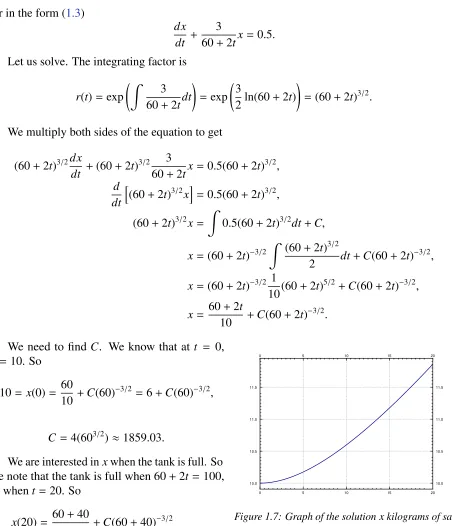
1.4. LINEAR EQUATIONS AND THE INTEGRATING FACTOR 35 Or in the form (1.3)

dx dt +

3

60+2tx=0.5. Let us solve. The integrating factor is

r(t)= exp

Z

3 60+2tdt

!

= exp 3

2ln(60+2t)

!

=(60+2t)3/2.

We multiply both sides of the equation to get

(60+2t)3/2dx

dt +(60+2t)

3/2 3

60+2tx=0.5(60+2t)

3/2_,

d dt

h

(60+2t)3/2xi =0.5(60+2t)3/2, (60+2t)3/2x=

Z

0.5(60+2t)3/2dt+C, x=(60+2t)−3/2

Z

(60+2t)3/2

2 dt+C(60+2t)

−3/2_,

x=(60+2t)−3/2 1

10(60+2t)

5/2₊

C(60+2t)−3/2, x= 60+2t

10 +C(60+2t)

−3/2_.

We need to find C. We know that at t = 0,

0 5 10 15 20

10.0 10.5 11.0 11.5

[image:35.612.82.534.99.625.2]

10.0 10.5 11.0 11.5

Figure 1.7: Graph of the solution x kilograms of salt in the tank at time t.

x=10. So 10= x(0)= 60

10 +C(60)

−3/2₌

6+C(60)−3/2, or

C =4(603/2)≈1859.03.

We are interested inxwhen the tank is full. So we note that the tank is full when 60+2t=100, or whent=20. So

x(20)= 60+40

10 +C(60+40)

−3/2

≈ 10+1859.03(100)−3/2 ≈11.86. See Figure 1.7for the graph ofxovert.

(36)

1.4.1

Exercises

In the exercises, feel free to leave answer as a definite integral if a closed form solution cannot be found. If you can find a closed form solution, you should give that.

Exercise1.4.4: Solve y0+ xy= x.

Exercise1.4.5: Solve y0+6y=ex.

Exercise1.4.6: Solve y0+_3x2_y= _sin(x)_e−x3_{, with y(0)}= _1.

Exercise1.4.7: Solve y0+cos(x)y=cos(x).

Exercise1.4.8: Solve _x21₊₁y

0₊

xy=3, with y(0)=0.

Exercise1.4.9: Suppose there are two lakes located on a stream. Clean water flows into the first lake, then the water from the first lake flows into the second lake, and then water from the second lake flows further downstream. The in and out flow from each lake is 500 liters per hour. The first lake contains 100 thousand liters of water and the second lake contains 200 thousand liters of water. A truck with 500 kg of toxic substance crashes into the first lake. Assume that the water is being continually mixed perfectly by the stream. a) Find the concentration of toxic substance as a function of time in both lakes. b) When will the concentration in the first lake be below 0.001 kg per liter? c) When will the concentration in the second lake be maximal?

Exercise1.4.10: Newton’s law of cooling states that dx_dt =−k(x−A)where x is the temperature, t is time, A is the ambient temperature, and k> 0is a constant. Suppose that A= A0cos(ωt)for

some constants A0 andω. That is, the ambient temperature oscillates (for example night and day

temperatures). a) Find the general solution. b) In the long term, will the initial conditions make much of a difference? Why or why not?

Exercise1.4.11: Initially 5 grams of salt are dissolved in 20 liters of water. Brine with concentration of salt 2 grams of salt per liter is added at a rate of 3 liters a minute. The tank is mixed well and is drained at 3 liters a minute. How long does the process have to continue until there are 20 grams of salt in the tank?

Exercise1.4.12: Initially a tank contains 10 liters of pure water. Brine of unknown (but constant) concentration of salt is flowing in at 1 liter per minute. The water is mixed well and drained at 1 liter per minute. In 20 minutes there are 15 grams of salt in the tank. What is the concentration of salt in the incoming brine?

Exercise1.4.101: Solve y0+3x2_y= _x2_.

(37)

1.4. LINEAR EQUATIONS AND THE INTEGRATING FACTOR 37

Exercise1.4.103: Suppose a water tank is being pumped out at 3L/_min_{. The water tank starts at 10 L}

of clean water. Water with toxic substance is flowing into the tank at 2L/_min_{, with concentration}_20tg/_L

at time t. When the tank is half empty, how many grams of toxic substance are in the tank (assuming perfect mixing)?

Exercise1.4.104: Suppose we have bacteria on a plate and suppose that we are slowly adding a toxic substance such that the rate of growth is slowing down. That is, suppose that dP_dt =(2−0.1t)P. If P(0)= 1000, find the population at t= 5.

(38)

1.5

Substitution

Note: 1 lecture, §1.6 in [EP], not in [BD]

Just as when solving integrals, one method to try is to change variables to end up with a simpler equation to solve.

1.5.1

Substitution

The equation

y0 =(x−y+1)2

is neither separable nor linear. What can we do? How about trying to change variables, so that in the new variables the equation is simpler. We use another variablev, which we treat as a function of x. Let us try

v= x−y+1.

We need to figure outy0 in terms ofv0,vand x. We differentiate (in x) to obtainv0 = 1−y0. So y0 =1−v0. We plug this into the equation to get

1−v0 = v2.

In other words,v0 = ₁₋_v2_{. Such an equation we know how to solve by separating variables:}

1

1−v2 dv= dx.

So

1 2ln

v+1 v−1

=

x+C,

v+1 v−1

=

e2x+2C,

or v_v−+1₁ = De2x for some constantD. Note thatv=1 andv=−1 are also solutions. Now we need to “unsubstitute” to obtain

x−y+2 x−y = De

2x_,

and also the two solutionsx−y+1=1 ory= x, andx−y+1=−1 ory= x+2. We solve the first equation fory.

x−y+2= (x−y)De2x, x−y+2= Dxe2x −yDe2x, −y+yDe2x = Dxe2x −x−2, y(−1+De2x)= Dxe2x −x−2,

y= Dxe

2x₋

(39)

1.5. SUBSTITUTION 39 Note thatD=0 givesy= x+2, but no value ofDgives the solutiony= x.

Substitution in differential equations is applied in much the same way that it is applied in calculus. You guess. Several different substitutions might work. There are some general patterns to look for. We summarize a few of these in a table.

When you see Try substituting yy0 _v=_y2

y2y0 v=y3 (cosy)y0 v=siny (siny)y0 _v=_cos_y

y0ey v=ey

Usually you try to substitute in the “most complicated” part of the equation with the hopes of simplifying it. The above table is just a rule of thumb. You might have to modify your guesses. If a substitution does not work (it does not make the equation any simpler), try a different one.

1.5.2

Bernoulli equations

There are some forms of equations where there is a general rule for substitution that always works. One such example is the so-calledBernoulli equation∗_:

y0+ p(x)y= q(x)yn.

This equation looks a lot like a linear equation except for theyn_{. If}_n=_{0 or}_n=_{1, then the equation}

is linear and we can solve it. Otherwise, the substitutionv= y1−ntransforms the Bernoulli equation into a linear equation. Note thatnneed not be an integer.

xy0+y(x+1)+xy5 =0, y(1)= 1.

First, the equation is Bernoulli (p(x)= (x+1)/xandq(x)= −1). We substitute v=y1−5 = y−4, v0 =−4y−5y0.

In other words, (−1/₄₎_y5_v0 = _y0_{. So}

xy0+y(x+1)+xy5 =0, −xy5

4 v

0₊

y(x+1)+xy5 =0, −x

4 v

0₊

y−4(x+1)+x=0, −x

4 v

0₊

v(x+1)+x=0,

∗_{There are several things called Bernoulli equations, this is just one of them. The Bernoullis were a prominent}

(40)

and finally

v0− 4(x+1) x v=4.

The equation is now linear. We can use the integrating factor method. In particular, we use formula (1.4). Let us assume thatx>0 so|x|= x. This assumption is OK, as our initial condition isx= 1. Let us compute the integrating factor. Here p(s) from formula (1.4) is −4(s_s+1).

e

Rx

1 p(s)ds= exp

Z x

1

−4(s+1) s ds

!

=e−4x−4 ln(x)+4 =e−4x+4x−4= e

−4x+4

x4 ,

e−

Rx

1 p(s)ds= e4x+4 ln(x)−4 =e4x−4x4.

We now plug in to (1.4)

v(x)= e−

Rx 1 p(s)ds

Z x

1

e

Rt

1 p(s)ds4dt+1

!

= e4x−4x4

Z x

1

4e

−4t+4

t4 dt+1 !

.

The integral in this expression is not possible to find in closed form. As we said before, it is perfectly fine to have a definite integral in our solution. Now “unsubstitute”

y−4 =e4x−4x4 4

Z x

1

e−4t+4 t4 dt+1

!

,

y= e

−x+1

x4Rx

1

e−4t+4

t4 dt+1

1/4.

1.5.3

Homogeneous equations

Another type of equations we can solve by substitution are the so-calledhomogeneous equations. Suppose that we can write the differential equation as

y0= F

_y

x

.

Here we try the substitutions v= y

x and therefore y

0 ₌

v+xv0.

We note that the equation is transformed into

v+xv0 = F(v) or xv0 = F(v)−v or v

0

(41)

1.5. SUBSTITUTION 41 Hence an implicit solution is

Z

1

F(v)−v dv=ln|x|+C. Example 1.5.2: Solve

x2y0 =y2+xy, y(1)=1.

We put the equation into the formy0 = (y/_x₎2+y/_x_{. We substitute} _v =y/_x _{to get the separable}

equation

xv0 = v2+v−v=v2, which has a solution

Z

1

v2 dv= ln|x|+C,

−1

v = ln|x|+C, v= −1

ln|x|+C. We unsubstitute

y x =

−1 ln|x|+C, y= −x

ln|x|+C. We wanty(1)= 1, so

1=y(1)= −1 ln|1|+C =

−1 C . ThusC = −1 and the solution we are looking for is

y= −x ln|x| −1.

1.5.4

Exercises

Hint: Answers need not always be in closed form.

Exercise1.5.1: Solve y0+y(x2−1)+xy6 =0, with y(1)= 1.

Exercise1.5.2: Solve2yy0₊₁₌

y2+x, with y(0)= 1.

Exercise1.5.3: Solve y0+ _xy=_y4_{, with y(0)}=_1.

(42)

Exercise1.5.5: Solve y0= (x+y−1)2.

Exercise1.5.6: Solve y0= x2_xy−y2, with y(1)=2.

Exercise1.5.101: Solve xy0+_y+_y2 =_{0, y(1)}=_2.

Exercise1.5.102: Solve xy0+y+x=0, y(1)=1.

Exercise1.5.103: Solve y2_y0 =_y3₋_{3x, y(0)}= _2.

Exercise1.5.104: Solve2yy0 = ey2−x2

(43)

1.6. AUTONOMOUS EQUATIONS 43

1.6

Autonomous equations

Let us consider problems of the form dx

dt = f(x),

where the derivative of solutions depends only onx(the dependent variable). Such equations are calledautonomous equations. If we think oftas time, the naming comes from the fact that the equation is independent of time.

Let us return to the cooling coffee problem (see Example 1.3.3). Newton’s law of cooling says dx

dt = −k(x−A),

where xis the temperature,tis time, kis some constant, and Ais the ambient temperature. See Figure 1.8for an example withk =0.3 and A=5.

Note the solutionx=A(in the figure x=5). We call these constant solutions theequilibrium solutions. The points on thexaxis where f(x) = 0 are calledcritical points. The point x= Ais a critical point. In fact, each critical point corresponds to an equilibrium solution. Note also, by looking at the graph, that the solutionx= Ais “stable” in that small perturbations in xdo not lead to substantially different solutions astgrows. If we change the initial condition a little bit, then as t→ ∞we get x(t)→ A. We call such critical pointsstable. In this simple example it turns out that all solutions in fact go toAast → ∞. If a critical point is not stable we would say it isunstable.

0 5 10 15 20

-10 -5 0 5 10

Figure 1.8: The slope field and some solutions of x0 =−0.3 (x−5).

0 5 10 15 20

-5.0 -2.5 0.0 2.5 5.0 7.5 10.0

Figure 1.9: The slope field and some solut