Quantum Algorithms for Universal Prediction

(1)

Quantum Algorithms for

Universal Prediction

Elliot Catt

(2)

(3)

Declaration

This thesis is an account of research undertaken between July 2017 and May 2018 at The Mathe-matical Sciences Institute, The Australian National University, Canberra, Australia.

Except where acknowledged in the customary manner, the material presented in this thesis is, to the best of my knowledge, original and has not been submitted in whole or part for a degree in any university.

Elliot James Carpenter Catt 24th May, 2018

Supervisor:

(4)

(5)

Acknowledgements

There are a lot of people I want to acknowledge, people who helped me, people who pushed me, people who made me who I am.

Marcus, thank you for working with me on this project. Thank you for always listening to my ideas, and in a lot of cases explaining why they wouldn’t work. Your comments constantly gave me ways to improve everything I wrote and came up with. You always gave good advice on everything I asked about, not limited to this project. You pushed me to work hard, to understand things in a deep way and above all else to do well. Thank you.

To Amy. Who I believe has read and proof read this thesis more than any other person, for that I thank you. Not only do you give me motivation and drive, your patience and caring are second to none. You listened to all my explanations, you commented and critiqued them, helping me understand my own ideas better through explanation. For these reasons and everything else, thank you.

To Cyril. Over my life no one has taught me as much as you. You taught me everything, from history to geography to science and mathematics to rhetoric, and so much more. I hope I can one day repay my debt to you. Thank you.

To Jon, you were the one who encouraged me to pursue research, you are the kind of researcher I want to be. Thank you for everything.

(6)

(7)

List of Figures

4.1 Deterministic Turing Machine . . . 32 4.2 Probabilistic Turing Machine . . . 32 4.3 Quantum Turing Machine . . . 32 4.4 Quantum Circuit for the Phase estimation algorithm (Nielsen and Chuang, 2002;

Wikipedia, 2017b) . . . 39 4.5 Quantum circuit for the Deutsch-Jozsa Algorithm (Nielsen and Chuang, 2002) . . . 41 4.6 Order finding quantum part of Shor’s algorithm (Nielsen and Chuang, 2002) . . . 44 4.7 Quantum circuit for Shor’s algorithm (Wikipedia, 2017c) . . . 44 4.8 Quantum Search Algorithm (Nielsen and Chuang, 2002) . . . 47 4.9 Quantum Circuit for Grover’s algorithm (Nielsen and Chuang, 2002; Wikipedia, 2017a) 47 4.10 Quantum Circuit for the Quantum Counting algorithm (Nielsen and Chuang, 2002;

(12)

(13)

List of Algorithms

1 Classical Order finding (Nielsen and Chuang, 2002) . . . 43

2 Classical Computable fixed-length speed prior algorithm . . . 60

3 Quantum Counting speed prior algorithm . . . 61

4 Quantum Speed prior algorithm . . . 63

(14)

(15)

Chapter 1

Introduction

Quantum Computing (QC) is a form of computation that has been shown to outperform classical computing on several tasks. These tasks include factoring numbers, querying databases, and some aspects of machine learning. There has been little work done on using Quantum Computing to achieve speedups in areas relevant to the study of inductive reasoning, reinforcement learning and algorithmic information theory.

By itself, inductive reasoning is a powerful tool that can solve a myriad of problems. One of the greatest of these, the problem of Artificial General Intelligence (AGI), is unlikely to be solved by inductive reasoning alone. Hutter (2005) presented a theoretical solution to the problem of AGI with the optimal agent AIXI. The agent AIXI is a combination of reinforcement learning and algorithmic information theory. AIXI is unfortunately incomputable, however it can be approximated. In this thesis we present Quantum Algorithms which improve on the classical method of approximating AIXI.

In Chapter 2, we will give a short description of the background required for this thesis; this includes computability, probability, and computational complexity theory. In Chapter 3, we will describe the problem of induction, specifically inductive reasoning, as well as some approaches to the problem of induction. This will include an explanation of Kolmogorov complexity and Solomonoff Induction.

In Chapter 4, we will describe quantum computing, from its inception to the present; the foundation of quantum complexity theory; advances in quantum computability; and some well-known quantum algorithms which provide large speedups over their classical counterparts.

In Chapter 5, we go over the hardness of counting, specifically the implications of a fast classical or quantum algorithm.

(16)

and go on to present two quantum algorithms to compute the Speed prior.

The advantage in using the quantum algorithms to compute the Speed prior is that there is a potential speedup in the time taken. The first quantum algorithm provides a quadratic speedup over the classical method, while the second provides an exponential speedup, however the approximation is more crude.

(17)

Chapter 2

Preliminaries

In this chapter we will cover some of the prerequisites of this thesis, namely the basics of probability, computability and complexity.

2.1 Probability

Probability is the study of events and their likelihoods. To describe later results we will need to define probability measures on binary strings. We use the notation for binary strings: B“ t0,1u,

B˚“Ť_nt0,1un, is the empty string, andB8 is the set of all one way infinite sequences ofB.

Definition 2.1.1 (Cylinder set (Li and Vit´anyi, 2014)). A cylinder set Γx ĎB8, for xPB˚, is

the set

Γx“ txω:ωPB8u

Let_G“ tΓx:xPB˚uthen a functionµ1_:

GÑRis defines a probability measure if

1. µ1

pΓq “1 2. µ1

pΓxq “ ÿ bPB˚

µ1

pΓxbq

We will use the notation whereµpxq “µ1_p_Γ_xq_{, then the definition of a measure can be written as}

Definition 2.1.2 (Probability Measure (Li and Vit´anyi, 2014)). The a function µ : _B˚ _Ñ

R is

defines a probability measure if

1. µpq “1 2. µpxq “ ÿ

(18)

Expected value is another tool from probability which we will be using.

Definition 2.1.3. Given a probability mass functionPpxqthe (discrete) expected value of a function

f is defined as follows

Erfs “ÿ x

fpxqPpxq (2.1)

An example of the expected value is given below,

Example 2.1.1. The expected value of the sum of rolling two fair 6-sided dice with the probability mass functionPpxq “1{36, the expected value formula gives us the following formula

ÿ

a,bPt1,2,3,4,5,6u

pa`bq ¨ 1

36 “7

2.2 Computability

First proposed by Alan Turing in Turing (1937), Turing machines are a class of machines with a tape of zeros and ones, a head which moves along and writes on the tape, and a program determining where the head should go. This simple form of computation is the foundation of computer science, which as a field could be described as “things that can be done with Turing machines”.

Turing machines are not the only form of computation, another equal form of computation is Lambda calculus (Church), which takes a much more functional (in the mathematical sense) approach to computing. Other forms of equivalent computation include (but are not limited to) partial recursive functions, register machines, and Markov algorithms. The idea that all forms of computation are “equivalent” is called the Church-Turing thesis.

Formally we define a Turing Machine as follows,

Definition 2.2.1 (Bernstein and Vazirani (1997)). A deterministic Turing machine is a triplet

pΣ, Q, δq, where Σis a finite alphabet with an identified blank symbol #,Q is a finite set of states with identified initial state q0 and finial stateqf‰q0, andδ, a deterministic transition function, is a function

δ : QˆΣÑΣˆQˆ tL, Ru (2.2)

Here tL, Rudenote left and right, directions to move on the tape. The state qf is also called the

Halting state.

Turing machines can be thought of as a head moving along an infinite tape, and on this tape are elements from the alphabet t#u YΣ. The head moves up and down the tape, and reads and writes according to the functionδ.

(19)

does halt, and outputs undefined if it does not halt. Hence being a partial function. When referring to the Turing machine as a function we will be referring to the δ˚ _{of that Turing machine.}

A configuration of a Turing machine, which is a current description of the Turing Machine is defined as follows

Definition 2.2.2(Configuration). A configuration (of a Turing Machine) is a tuplepd, h, qqwhere

dis a description of the contents of the tape, his the location of the head symbol, andq represents the state the Turing machine is in.

To receive an output on our computation we require the Turing machine to halt, that is, even-tually enter the final stateqf. Unfortunately this is not always the case. For example consider the

machines below,

Example 2.2.1.

Σ“ t#,1u

Q“ pq0, qfq

δpq0,#q “ p1, q0, Rq

δpq0,1q “ p1, q0, Rq

This machine writes 1, then moves right forever. It will never halt since the functionδnever maps to the stateqf. Below is the state diagram of this Turing machine,

q0 qf

δpq0,#q

δpq0,1q

A non-halting machine may not use an infinite amount of tape, as seen in the next example.

Example 2.2.2.

Σ“ t#,1u

Q“ pq0, q1, qfq

δpq1,#q “ p1, q0, Lq

δpq1,1q “ p1, q0, Lq

(20)

q0 q1 qf

δpq0,1q

δpq0,#q

δpq1,1q

δpq1,#q

Turing machines can also be viewed as functions equivalent to partial recursive functions Boolos et al. (2002).

The ‘Halting problem’ is determining whether or not a Turing machine will halt on a given input. Turing proved that one cannot in fact use a Turing machine to determine that another Turing machine will not halt on any input.

Theorem 2.2.1 (Halting problem). There does not exist a Turing Machine which can determine if a given Turing Machine will not halt on any input.

The ‘Halting problem’ is a good example of something which is incomputable: it is something which no Turing machine can compute.

2.3 Complexity Theory

Complexity theory is the study of how long it takes to compute a function on a Turing machine. Specifically, given a Turing machine (which is representing a functionδ˚_{), how many steps does} the Turing machine take to compute that function in terms of the size of the input of the Turing machine.

(21)

Example 2.3.1.

Σ“ t#,1u

Q“ pq0, q1, q2, qfq

δpq1,#q “ p#, q2, Lq

δpq2,1q “ p#, qf, Rq

The ADD Turing machine takes an input of two unary numbers separated by a #, p1l_#1m_{, then}

returns the sum of those two numbers,p1l`m

q. Below is the state diagram of this Turing machine,

q0 q1 q2 qf

δpq0,1q

δpq0,#q

δpq1,1q

δpq1,#q δpq2,1q

One can see that if the length of the numbers isn“l`m`1, then the number of steps required to compute this ADD function isn`2. In complexity theory, the big O notation is used to describe the time taken.

Definition 2.3.1. A function f is f P Opgq (read as big O of g) if Dc P R and n0 such that

|fpnq| ďc|gpnq|for all nąn0. We represent this by the notationfpnq “Opgpnqq.

From our previous example we would say the ADD function isOpnq, since there exists ac“2 and an0“4 such thatn`3ă2nfor allną4. A problem is said to be solved in polynomial time

if there exists a function which solves the problem and takes timeOpfpnqq, wheref is a polynomial of the size of the inputn. Similarly a problem is said to be solved in exponential time if there exists a function which solves the problem and takes timeOpfpnqq, wheref is an exponential function of the size of the inputn.

The two most important classes in complexity theory arePandNP. The classPis the class of all problems that can be solved in polynomial time; the classNPis the class of all problems that can be verified in polynomial time. Verifying a problem is being given a solution to the problem and checking if it is correct. For example if the problem was add 4 and 5, then we could be given a solution, such as 10 and we have to check if it is correct. In this case it is not.

The most famous problem in complexity theory is whether or notP“NP. This is essentially asking if being able to verify a problem in polynomial time implies we can solve the problem in polynomial time.

The reason these classes, and the above question, are so important comes down to the fact that

(22)

contains many problems which we cannot efficiently solve. Additionally several of these hard-to-solve problems are very relevant, for example the travelling salesman problem, protein folding, and RSA cryptography.

A problemB can be reduced in polynomial time to another problemAif there exists transfor-mation which takes at most polynomial time and transforms every instance of a problemBinto an instance of the problemA such that the transformation of the solution to the instance of the new problem A is the solution to the instance of the problemB. For example, any hamiltonian cycle problem can be reduced to a travelling salesman problem by giving all the edges of the hamiltonian cycle problem weight 1, and creating edges with weight 2 where all the non existent edges of the hamiltonian cycle problem are. The solution to the resulting travelling salesman problem can be transformed to the solution to the initial hamiltonian cycle problem, and the transformation takes at msot polynomial time.

If every problem inNP can be reduced in polynomial time to a problem A, then we sayA is

(23)

Chapter 3

Induction

3.1 Introduction to Induction

The problem of induction, specifically inductive reasoning, is one of the most well-studied problems in philosophy (De Finetti, 1972; Popper, 1957, 1985; Hume, 2000; Cohen, 1989; Carnap, 1962). First discussed in Hume (1738), the problem of induction and inductive reasoning is the process of reasoning about a hypothesis, given some evidence (data). Outside of philosophy, many areas such as machine learning, statistics, and economics, rely heavily on induction and have produced many practical solutions to the problem. This is because induction can be used to find “truth” in the world. Inductive ability has also for a long time been the way in which we test a human’s ability, in the form of IQ tests, and many similar examinations.

Many of the aforementioned studies have proposed solutions to the induction problem, some of which have found great practical success such as Nasrabadi (2007) in statistical machine learning. One proposed solution to the Induction problem, Solomonoff induction (Solomonoff, 1964a), has benefits over all other solutions (as well as some downsides); this will be the focus of this chapter.

3.2 Approaches to Induction

3.2.1 Laplace/Bayesian Approach

Laplace’s approach to the induction problem is a rule of succession (Solomonoff, 1964a), also called Bayes-Laplace estimator. This rule was famously demonstrated with the problem of predicting whether or not the sun would rise tomorrow. The following explanation is from Hutter (2005).

(24)

Theorem 3.2.1 (Bayes’ Theorem). Let H andD be events, then

PpH|Dq “PpD|HqPpHq

PpDq

WherePpHqbe the prior plausibility of the hypothesisH,PpD|Hqis the likelihood of the data D under the hypothesisH, andPpH|Dqis the posterior plausibility of of hypothesisH, andtHiu

form an exclusive and exhaustive set of hypothesis’. We also have PpDq “ ř_iPpD|HiqPpHiq. Then Bayes’ theorem in its most useful form

Theorem 3.2.2 (Bayes’ Rule).

PpH|Dq “ řPpD|HqPpHq

iPpD|HiqPpHiq

.

Using Bayes’ rule, one can use the prior probability to calculate the posterior plausibility of of hypothesis H given some data D, and this in turn can be used for inductive reasoning and prediction.

Getting back to predicting whether or not the sun will rise tomorrow. Let x be some finite binary sequence,x“x1. . . xnPBn, and letn0andn1be the number of 0’s and 1’s in the sequence

respectively. Let each element finite sequence be generated by some probability θP r0,1s, that is, Ppxi “ 1q “ θ for all i. Our hypothesis class is then Hθ “ Bernoullipθq. The likelihood of an

event y be given a hypothesis is Ppy|Hθq “ θn1_p₁_´_θ_qn0_{, and using a uniform prior plausibility} Ppθq “ PpHθq “ 1. Lastly the probability of some evidence Ppyq “ n1!n0!

pn`1q!. All together with

Bayes’ rule we get

Ppy|xq “ Ppx|yqPpyq

Ppxq “

pn`1q! n1!n0!

θn1_p₁_´_θ_qn0

Then if we let xi “ 1 if the sun rose on the ith day according to our data, we want to find the

probability of the the sun will rise tomorrow. Our data says that the sun rose for every previous day, then we get

Pp1|xq “Ppx1q

Ppxq “

n1`1

n`2 Which translates to

Ppsunrise tomorrow|all previous sunrisesq “ #days the sun has risen`1

#days the sun has risen`2.

So according to Bayes’ and Laplace’s rule if the sun has risen for 1012 _{days (the approximate age}

of the earth) then the probability the sun will not rise tomorrow is 1 1012_`₂.

3.3 Algorithmic Complexity and Solomonoff Induction

(25)

we will use the following notation. Let _B˚ _{denote the set of all finite binary strings, and let}_`_p_p_q denote the length of a binary string pPB˚.

Kolmogorov (1963) proposed a complexity measure of how complex a given string (or number) is. It is the length of the smallest program which when inputted into a (often Universal) Turing machine will produce the string. More formally,

Definition 3.3.1. Given a Turing machineT, the Kolmogorov complexity of a stringxis

KTpxq “min

p t`ppq : Tppq “xu

There has been much work done on Kolmogorov complexity, and its application to Artificial Intelligence, as well as to compression. For a detailed description on these topics and the properties of Kolmogorov complexity, see Hutter (2005). Although Kolmogorov complexity is incomputable, it is limit computable. A function fpxq is limit computable if there exists a computable function

ˆ

fpx, tqsuch thatfpxq “limtÑ8fˆpx, tq. This incomputabiliy comes from the fact that the programs being checked may not halt, and there is no way to determine which programs will not halt.

The problem of induction, that is, predicting or inferring what will come next given some past data, has been extensively studied. In 1964 Solomonoff proposed a solution to the induction problem (Solomonoff, 1964a,b).

Solomonoff Induction is based on Epicurus’ principle of multiple explanations and Occam’s Razor. Together these principles state that one should always consider every theory (or model) which is consistent with the data, however give preference to more simple theories (or models). Solomonoff represents the concept of complexity of a model by the length of a program which ‘computes’ the model.

Solomonoff (1964a,b) proposed four equivalent solutions to the induction problem, then demon-strated these induction techniques on three different induction tasks. The three induction tasks were induction on a Bernoulli sequence, induction on sequences with symbol constraints, and phrase structure grammars in coding for induction. Since the original paper the definition has been refined, and more applications have been demonstrated.

A description of Solomonoff Induction is as follows.

Definition 3.3.2. Given a universal monotone Turing Machine U, the universal (Solomonoff ) a-priori probability semi-measure ofxPB˚ is defined as

Mpxq “ ÿ p : Uppq“x˚

2´`ppq

wherex˚ denotes a string which starts withx.

The programs being summed over in the universal a-priori probability represent descriptions of x, and the 2´`ppq_{is a weight on the complexity of the description. In this way we define complexity} as description length. This is universal in the sense that every program is considered.

(26)

Definition 3.3.3. The corresponding conditional probability ofxgiveny is

Mpx|yq “ Mpyxq

Mpyq “

ř

p:Uppq“yx˚2 ´`ppq

ř

p:Uppq“y˚2´

`ppq

whereyx denotes the concatenation ofy with x.

As an example of this induction,

Example 3.3.1. If 0 denotes rainy and 1 denotes sunny and we wish to calculate the probability it will be sunny given the past data 0101000, we calculate

Mp1|0101000q “Mp01010001q

Mp0101000q “

ř

p:Uppq“01010001˚2 ´`ppq

ř

p:Uppq“0101000˚2´

`ppq

M is a universal semi-measure (Li and Vit´anyi, 2014) and, like Kolmogorov complexity, it is incomputable. The incomputability comes from the fact that one cannot compute every possible program on a universal Turing machine as some may not halt. Additionally it is required that every program be ran. Whereas for Kolmogorov complexity, one can show that only a finite amount of programs need to be ran. However, even though it it incomputable, it has been shown thatM is limit computable and there are algorithms which can approximate it. This will be discussed further in later sections.

The importance ofM comes from the following theorem proved by Solomonoff (1978), that is, Solomonoff induction.

Theorem 3.3.1 (Solomonoff (1978)). Let µ be a computable measure with x1, x2, . . . distributed according to µ. Then the total squared error between M andµwill be finite, specifically

Eµ

˜₈ ÿ

t“1

pMpxt`1“1|x1. . . xtq ´µpxt`1“1|x1. . . xtqq2

¸

ďKpµqlnp2q

2 ă 8

where Kpµq denotes the Kolmogorov complexity ofµ. This theorem states that the expected value of the sum of the squares of the difference between M and µ is bounded by a constant. Hence for any computable measureµ, Solomonoff’s prior will have a bounded error in prediction. Moreover it has been shown that any probability distribution P that satisfies Theorem 3.3.1 in place of M must be incomputable Solomonoff (2003). This shows that the incomputability ofM is not a bane but a requirement to be able to have bounded errors. In turn this demonstrates that any computable statistical procedure used in practice must have infinitely many errors on some sequences.

(27)

had, for a long time, been completely absent of any notion of probability. However, to be able to solve the big problem, that is the creation of strong (general) Artificial Intelligence, one must inevitably use probability. For a description of how Solomonoff Induction can be used to create a theoretically optimal agent for reinforcement learning, that is a (theoretical) strong Artificial Intelligence, see Hutter (2005) and Section 3.5.

3.4 Approximation schemes for Solomonoff Induction

There are algorithms which can approximate Kolmogorov complexity and the Solomonoff prior, most notably Levin search (Levin, 1973), Hutter search (Hutter, 2002), and the Optimal Order Problem solver (Schmidhuber, 2004).

Levin search (Levin, 1973) is an algorithm for solving a given inversion problem. Given a functionf and a valuey, the Levin search algorithm inverts the functionf. Levin search setsi:“0 and executes every input to the function, xPB˚, with `pxq ďi for time 2i₂´`pxq_{steps, then sets} i:“i`1 and repeats, until anxis found such thatfpxq “y.

Hutter Search (Hutter, 2002) is a general speedup algorithm for any given problem. It works by performing three different tasks and sharing resources between them. The first task is to prove that other functions (programs in a universal Turing machine) are equivalent to the desired program and that these functions have time bounds, all of this in formal logic. The second task is to compute the time bound of every program which satisfies the condition of the first task, and this computation is split up in a similar way to Levin Search. The third task is to run the function (program) which has the best time bound from the second task.

The G¨odel machine (Schmidhuber, 2007) is a self-improving solver. It works by first solving (some) problems, then while solving new problems searching for other solvers that are able to out-perform itself, and changing its own solver to the new solver when it finds a superior one.

3.5 The optimal agent AIXI

(28)

Agent Env Actions

Rewards

Observations

Solomonoff Induction and reinforcement learning can be used together to construct the optimal agent AIXI (Hutter, 2000). The agent AIXI, described in (Hutter, 2005), is optimal in the sense that there does not exist another agent which performs better than AIXI in all possible environments.

Given the historyo1r1. . . ok´1rk´1 where oi is the observation at the ith time step, andri is

the reward at theith time step, AIXI takes actionak defined by

ak:“arg max ak

ÿ

okrk

. . .max

am

ÿ

omrm

rrk`. . . rms

ÿ

q:Upq,a1...amq“o1r1...omrm

2´`pqq _(3.1)

(29)

Chapter 4

Quantum Computing

(30)

4.1 Introduction

The central idea in Quantum Computing (QC) is to use the quantum nature of the universe to provide speedups in computation that would otherwise be impossible in classical computing (Feyn-man, 1982). The physical realisation of this is called quantum supremacy (Aaronson and Chen, 2016). This quantum supremacy relies on two key features: first, a physically constructed quantum computer, and second, a Quantum algorithm running on the quantum computer that is beyond any (current) classical computation. We will be focusing on the quantum algorithm side. A complete description of the physical and algorithmic aspects of quantum computing can be found in Nielsen and Chuang (2002).

There are two ways in which we will describe quantum computation: first, the way in which it was established, as quantum Turing machines. Second, quantum Circuits, which give a clear description of quantum algorithms. It has been shown that these are equivalent by Yao (1993).

4.2 Quantum Turing Machines

The first formal definition of a Quantum Turing Machine (QTM) is from Deutsch (1985). A main topic of Deutsch (1985), and an important aspect of the purpose of quantum computing was the Church-Turing thesis and its expanded form, which we will discuss here before we get to the exact definition of Quantum Turing Machines.

4.2.1 Church-Turing Thesis

The Church-Turing thesis is as follows:

Every ‘function which could be regarded as computable’ can be computed by a universal Turing Machine.

This states that anything which we may wish to compute could be simulated on a universal Turing machine. However it does not mention anything about the time it would take for the universal Turing machine to simulate a computation.

Deutsch proposed a new version of the thesis, reflecting the physical nature of reality, now called the Church-Turing-Deutsch thesis.

Every finitely realisable physical system can be perfectly simulated by a universal model computing machine operating by finite means.

(31)

we can (quite easily) construct functions that are theoretically possible to compute with a Turing machine, however the functions are not representing any finitely realisable physical system. The constraint here is physical, as the time required to compute some functions is greater than the heat-death of the universe: For example, the Ackermann function (Calude et al., 1979).

Lastly from Complexity theory, there is the related Extended-Church-Turing thesis by Kaye et al. (2007):

A probabilistic Turing machine can efficiently simulate any realistic model of computa-tion.

With the inclusion of “efficiently”, one excludes a large number of problems which are both com-putable and also represent finitely realisable physical systems. It is important to note that if quantum computing became a “realistic model of computation”, then this thesis may be negated, since probabilistic Turing machines cannot efficiently simulate quantum Turing machines.

4.2.2 Formalising Quantum Turing Machines

In a certain sense, a quantum Turing machine is essentially a probabilistic Turing machine which uses the L2 _{norm instead of the} _L1 _{norm; has complex-valued amplitudes in the place of}

non-negative real probabilities; and a complex-valued unitary transition matrix instead of a stochastic one. This is similar to how quantum mechanics, without the physics, is (essentially) probability theory with theL2 _{norm (Aaronson, 2013).}

With a classical (deterministic) Turing machine, the actions performed and state transitions are unsurprisingly deterministic; this means what we expect to happen will exactly happen. With a classical probabilistic Turing machine, each action will occur with some (non-negative) real proba-bility. This means that the machine could write 0 with some probability pand write 1 with some other probabilityq. As mentioned above, a quantum Turing machine is quite similar, except instead of (non-negative) real probabilities, the quantum Turing machine uses complex-valued amplitudes, where the sum of the squares of the absolute value of the amplitudes must be 1 at all times.

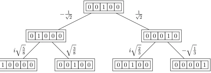
It can help to think of this kind of computation as a tree, where each node is a configuration of the quantum Turing machine. The branch width of this tree is the number of possible actions and the depth is the number of actions taken. At each time step, we move down the tree according to the unitary transition matrix.

(32)

0 0 1 0 0

0 0 0 1 0

0 0 0 0 1 0 0 1 0 0

1 0

0 1 0 0 0

0 0 1 0 0 1 0 0 0 0

1 0

[image:32.612.113.454.90.211.2]

0 1

Figure 4.1: Deterministic Turing Machine

Then the Probabilistic Turing machine. Note that at each vertex the branching edges must add to 1.

0 0 1 0 0

0 0 0 1 0

0 0 0 0 1 0 0 1 0 0

2 3

1 3

0 1 0 0 0

0 0 1 0 0 1 0 0 0 0

[image:32.612.115.453.286.405.2]

5 8 3 8 1 2 1 2

Figure 4.2: Probabilistic Turing Machine

Lastly the Quantum Turing Machine. Note here that the sum of the squared absolute value at each vertex of the branches must add to 1.

0 0 1 0 0

0 0 0 1 0

0 0 0 0 1 0 0 1 0 0

i b 2 3 ´ b 1 3

0 1 0 0 0

0 0 1 0 0 1 0 0 0 0

i b 5 8 b 3 8

´?1

2

1

?

2

Figure 4.3: Quantum Turing Machine

[image:32.612.115.453.480.598.2]

(33)

separate branches may have the same configuration. In the above examples, it is represented in the probabilistic Turing machine by the configuration 0 0 1 0 0 occurring with probability

1 2¨ 3 8` 1 2¨ 2 3 “ 19

48, and similarly for the quantum Turing machine, the configuration 0 0 1 0 0

occurring with amplitude´?1

2 ¨ b 3 8` 1 ?

2¨i

b

2

3 “ ´

b

3 16 `i

1

?

3. This addition of different paths

to the same configuration is quintessential to all Quantum algorithms.

Before formally defining the quantum Turing machine, we need to define the subset of the complex numbers that define the quantum Turing machine. Let ˜Cbe the set of complex numbers

αPCfor which there is a deterministic algorithm that computes the real and imaginary parts ofα

with an error of at most 2´n _{in time that is a polynomial of}_n_.

Additionally, recall that a configuration in Definition 2.2.2 is the combination of the tape, state and head position of a Turing Machine. Now we can formally define quantum Turing machines.

Definition 4.2.1 (Bernstein and Vazirani (1997)). A Quantum Turing Machine M is defined, much like a classical Turing Machine (Definition 2.2.1), by a triplet pΣ, Q, δq where Σ is a finite alphabet with an identified blank symbol (#), Qis a finite set of states with identified initial state

q0 and final stateqf ‰q0, andδ, the quantum transition function,

δ : Q ˆΣ Ñ C˜Σˆ Qˆ tL,Ru.

The QTMM has a two-way infinite tape of cells indexed by_Z, each holding symbols fromΣ, and a single read/write tape head that moves along the tape. A configuration or instantaneous description of the QTM is a complete description of the contents of the tape, the location of the tape head, and the state qPQof the finite control.

Let S be the inner-product space of finite complex linear combinations of configurations of M

with the Euclidean norm. We call each element φPS a superposition ofM.

φ“ÿ i

αimi

The QTM M defines a linear operator UM :S ÑS, called the time evolution operator of M, as

follows: if M starts in configuration c with current state qk, and scans symbol a, then after one

stepM will be in a superposition of configurationsψ“ř_iαici, where each nonzeroαi corresponds

to a transition δpqk, a, b, qj, dq, andci is the new configuration (Definition 2.2.2) that results from

applying this transform to c. Extending this map to the entire space S through linearity gives the time evolution operatorUM.

However instead of using Quantum Turing machines to define our Quantum Computation, we will instead mainly use Quantum Circuits.

4.3 Quantum Circuits

(34)

Turing machines, in the sense that one can simulate the other with a polynomial slowdown. This equivalence was also demonstrated by Nishimura and Ozawa (2009).

Quantum circuits can be thought of as classical Boolean circuits, except instead of the classical bits which take values 0 and 1 (False and True), a quantum circuit uses qubits, where each qubit takes a value in a complex superposition of 0 and 1. We can represent this as a pair of amplitudes

pα, βq PC2 which has the property|α|2` |β|2“1. Hereαis representing the amplitude (complex probability) of being 0, andβ likewise for 1. We will use the bra-ket notation to describe qubits.

4.3.1 Bra-ket notation

The Dirac bra-ket (Dirac, 1939) notation is as follows: first we use it to represent the standard basis vectors of_C2

|0y “

ˆ

1 0

˙

, |1y “

ˆ

0 1

˙

with a single qubit being described as

|φy “α|0y `β|1y “

ˆ

α β

˙

.

This asymmetrical notation is called a ket. This choice of notation is far less cumbersome than regular vector notation.

For|ay “

ˆ

α0

α1

˙

and|by “

ˆ

β0

β1

˙

,

we will also define the tensor product in bra-ket notation as follows:

|ay b |by “ |ay |by “ |aby “

¨ ˚ ˚ ˝

α0β0

α0β1

α1β0

α1β1

˛ ‹ ‹ ‚

For example, instead of writing|0y b |0y b |1ywe will write

|001y “

ˆ 1 0 ˙ b ˆ 1 0 ˙ b ˆ 0 1 ˙ “ ¨ ˚ ˚ ˚ ˚ ˚ ˚ ˚ ˚ ˚ ˚ ˝

1¨1¨0 1¨1¨1 1¨0¨0 1¨0¨1 0¨1¨0 0¨1¨1 0¨0¨0 0¨0¨1

(35)

We will also raise some qubits to the power of tensors, for example:

|ayb4“ |ay b |ay b |ay b |ay “ pαi, αj, αk, αlqi,j,k,lPt0,1u4

Additionally we will define the conjugate transpose as

xa| “ |ay: “ pα¯0,α¯1q

where ¯αis the complex conjugate ofα. This notation is called a bra. Using the two together we can write the inner product as

xa| |by “ xa|by “α¯0β0`α¯1β1

and the outer product as

|by xa| “

ˆ

β0α¯0 β0α¯1

β1α¯0 β1α¯1

˙

This is not the only notation that is used in Quantum computing, however this notation is the most simple and more importantly it is short.

4.3.2 Quantum Gates

Continuing this notation we can then represent quantum gates as matrices (transforms) which are applied to a superposition of qubits. It is important that they take a (collection of) qubits from one superposition to another. Specifically, it is required that the quantum gate conserves the }α}2₂“1 property.

So a matrix that conserves the superposition is unitary, i.e., its inverse is also its conjugate transpose. This is no surprise, since the state transition matrices of quantum physics must also be unitary. It has been shown that if any linear matrix was allowed, quantum computing would be unreasonably powerful (Aaronson, 2005).

Here we will define some of the common quantum gates used. This is not an exhaustive list. The ones we will define are the Hadamard gate, the π{8 (rotation) gate, and the controlled-not gate.

Definition 4.3.1. The Hadamard gate H acts on a single qubit and corresponds to the following unitary matrix

H“ ?1

2

ˆ

1 1

1 ´1

˙

.

For instanceH|0y “ˇˇ1₂ D

:“ ?1

2

ˆ

1 1

˙

andHH|0y “H?1

2

ˆ

1 1

˙

“ |0y.

(36)

Definition 4.3.2. The controlled-not gate, CN OT, acts on two qubits and performs the not (bit flip) operation on the second qubit if the first qubit is |1y. This equates to the following unitary matrix

CN OT “

¨ ˚ ˚ ˝

1 0 0 0 0 1 0 0 0 0 0 1 0 0 1 0

˛ ‹ ‹ ‚

.

For instanceCN OT|0y |ay “ |0y |ayandCN OT|1y |ay “ |1y b

ˆ

α0

α1

˙

Definition 4.3.3. The π{8 gate, Rπ{4, corresponds to a rotation of the |1y qubit by π{4. The matrix representing this rotation is

Rπ{4“

ˆ

1 0

0 eiπ4

˙

, Rπ{4|ay “

ˆ

α0

α1ei

π

4

˙

.

The gate is called the π{8 gate for historical reasons, even though the gate is a rotation of π{4. These three gates are important as they form a universal set of gates for two qubits. This means that any classical two bit circuit can be constructed using only these three gates (Nielsen and Chuang, 2002).

When working with larger numbers of qubits, to apply one of the above transforms to just some of the qubits, we use identity matrices with block-diagonal matrices of the transform(s).

For example if given two qubits, we wish to apply the Hadamard transform to only the second one, we can use the following matrix

H1“Hb

ˆ

1 0 0 1

˙

This process can be used for any number of qubits.

4.3.3 Measurement

Now that we have qubits and quantum gates, we need a way to measure the outcome. We call this quantum measurement. This measurement is done according to theL2 _{norm; for a system of}

the form ř2_xn_“´₀1αx|xy, we will observexwith probability|αx|2. Specifically, measurement of an n qubit system will do the following:

2n_´₁

ÿ

x“0

αx|xy Ñi with probability |αi|2

(37)

Additionally, one can choose instead to measure a subset of the quantum circuit, for example the firstmqubits. This is no different from the regular measurement, except that the observer will not gain any information about then´mqubits remaining.

In several quantum computations one uses extra qubits to aid in the computation which are not measured at the end of the computation.

It is important to note that this is destructive measurement. This means that performing the measurement will destroy the superposition of the system.

Although we can only ensure an outcome with some probability, we can repeat the computation and reduce the probability of error exponentially. Ultimately, we will only ever be sure of an outcome with some (quite high) probability. In most cases this is good enough.

When performing analysis of a quantum algorithm, it is important to include the number of times the computation must be repeated to reduce the error sufficiently, since this will increase the time complexity (potentially exponentially if it is required to be repeated an exponential number of times).

To give some examples of full quantum circuits, it will be useful to demonstrate some essential quantum algorithms.

4.3.4 Submodules

In this section we will explain the building blocks of quantum algorithms.

Quantum Oracle

The quantum oracle is used when we want to apply a functionf :t0,1unÑ t0,1uto a superposition of all elements of t0,1un. Since all transforms in quantum computing are reversible (and indeed unitary) there needs to be some way to keep the information so that the transform can be reversed. Classically we could takexÑfpxq, however when performing this transform in quantum computing we do the following

Uf|xy |yy “ |xy |y‘fpxqy.

Wherey is representing an extra qubit used for this reversibility.

Quantum Fourier Transform

(38)

on a vector|jy of size 2n _{as follows,}

QF T |jy “ 1

2n{2 2n_´₁

ÿ

k“0

e2πijk{2n

|ky. (4.1)

An expanded representation of the quantum Fourier transform, into the binary expression of j“j1j2. . . jn, is

|jy Ñ 1

2n{2

`

|0y `e2πi0.jn_|₁_y˘ `_|₀_{y `}_e2πi0.jn´1jn_|₁_y˘_{. . .}`_|₀_{y `}_e2πi0.j1...jn_|₁_y˘_. _(4.2)

Here 0.jn is thenth binary digit ofj divided by 2, likewise for 0.jn´1jn and 0.j1. . . jn.

The unitary matrix form of the QF T of n qubits is a matrix QF T “ ?1

2npaijq with entries

aij “ωpi´1qpj´1q, whereω is the 2nth root of unity.

Inverse Quantum Fourier Transform

Also somewhat unsurprisingly the inverse quantum Fourier transform (QF T´1_{) is the inverse of}

the quantum Fourier transform. That is,QF T QF T´1

“QF T´1 QF T “I the identity.

QF T´1

˜

1 2n{2

2n_´₁

ÿ

k“0

e´2πijk{2n

|ky

¸

“ |jy (4.3)

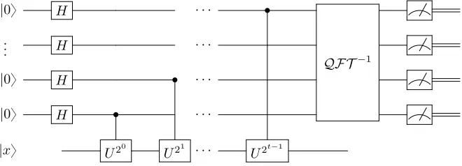
Phase Estimation

Given a unitary transform U with an eigenvector |xy and an eigenvalue e2πiω_{, phase estimation,}

as described in Nielsen and Chuang (2002), allows us to estimate the value of ω. The algorithm operates on two registers, first a register of t qubits, where t depends on the number of bits of accuracy required and the probability of success required. Specifically, for accuracy of m and probability of success 1´, we chooset“m`rlogp2`₂1qs. The second register is|xy. The algorithm has four steps, first performing the Hadamard operation on the first register; then performing a controlled version of the unitary operation U on the first register; then performing the inverse Fourier transform, as mentioned above, on the first register; then lastly performing measurement on the first register.

(39)

above are as follows,

|0ybt|xy Ñ 1

2t{2 2t´1

ÿ

k“0

|ky |xy Hadamard

Ñ 1

2t{2 2t_´₁

ÿ

k“0

e2πiωk|ky |xy Controlled-U

“ 1

2t{2

´

|0y `e2πi2t´1ω|1y

¯ ´

|0y `e2πi2t´2ω|1y

¯

. . .

´

|0y `e2πi20ω|1y

¯

|xy

“ 1

2t{2

`

|0y `e2πi0.ωt_|₁_y˘ `_|₀_{y `}_e2πi0.ωt´1ωt_|₁_y˘

. . .`|0y `e2πi0.ω1...ωt_|₁_y˘_|_x_y

Ñ |ω˜y |xy Inverse Fourier transform

Ñω˜ Measurement on first register

The Quantum circuit for Phase estimation is as follows,

|0y H ¨ ¨ ¨ ‚

QF T´1

..

. H ¨ ¨ ¨

|0y H ‚ ¨ ¨ ¨

[image:39.612.115.445.338.457.2]

|xy _U20 _U21 _{¨ ¨ ¨} _U2t´1

Figure 4.4: Quantum Circuit for the Phase estimation algorithm (Nielsen and Chuang, 2002; Wikipedia, 2017b)

Phase estimation is an essential part of the Quantum Counting Algorithm and many other quantum algorithms.

4.4 Quantum Algorithms

In this section we will describe some quantum algorithms. The general setup of all of these algo-rithms is as follows:

(40)

• Quantumize to create a uniform superposition over all possible qubits, often done with the Hadamard gateHbn

• Perform computation of some function in simultaneous states of this superposition

• Uncompute the superposition, often done with the Hadamard gate or the inverse Quantum Fourier transform

• Measurement of some or all of the circuit

We will first describe the setup of each algorithm, then give an intuitive explanation to each and why they are superior to their classical counterpart. This will be followed by a formal algebraic description of the algorithms, then a demonstration of the quantum circuit that would be used. This is by no means a complete list of Quantum algorithms; it is however a list of all algorithms which are relevant to this thesis.

4.4.1 Deutsch-Jozsa Algorithm

The Deutsch-Jozsa Algorithm is the first example of an exponential “quantum-speedup”. Imagine we are given a function f : t0,1un Ñ t0,1uthat has the property that either all values map to 0, or half of them do. Our objective is to determine whether every value maps to 0, or half of them do. To check this classically, one must perform at most 2n´1

`1 function evaluations. This is because the moment the function outputs a 1 we know thatf outputs 1 on half the inputs. The Deutsch-Jozsa Algorithm requires only 1 function evaluation.

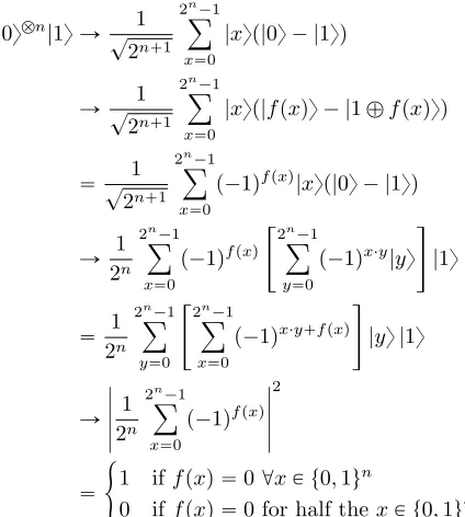
An exponential speedup comes from evaluating the function in a superposition of every input. To achieve this, we use the Hadamard gate which takes the initial state to a superposition of every possible state, with equal amplitude. Then we use oracle (function)f once in the oracle transform Uf which is defined as follows:

Uf|xy |yy “ |xy |y‘fpxqy

(41)

|0ybn|1y Ñ ? 1

2n`1 2n_´₁

ÿ

x“0

|xyp|0y ´ |1yq HadamardHbn bH

Ñ? 1

2n`1 2n´1

ÿ

x“0

|xyp|fpxqy ´ |1‘fpxqyq f oracle

“? 1

2n`1 2n_´₁

ÿ

x“0

p´1qfpxq|xyp|0y ´ |1yq sincefpxq “0,1

Ñ 1

2n

2n_´₁

ÿ

x“0

p´1qfpxq

«₂n_´₁

ÿ

y“0

p´1qx¨y|yy

ff

|1y HadamardHbn

bH

“ 1

2n

2n´1

ÿ

y“0

«₂n

´1

ÿ

x“0

p´1qx¨y`fpxq

ff

|yy |1y Re-ordering

Ñ ˇ ˇ ˇ ˇ ˇ 1 2n

2n_´₁

ÿ

x“0

p´1qfpxq

ˇ ˇ ˇ ˇ ˇ 2

Measurement on firstnqubits

“

#

1 iffpxq “0 @xP t0,1un

0 iffpxq “0 for half thexP t0,1un

The quantum circuit below is exactly the transforms described above.

|0y {n Hbn

Uf

Hbn

[image:41.612.101.313.112.348.2]

|1y H

Figure 4.5: Quantum circuit for the Deutsch-Jozsa Algorithm (Nielsen and Chuang, 2002)

It is important to note that one may use the Deutsch-Jozsa Algorithm with an oracle f :

t0,1unÑ t0,1ufor which the proportion of inputs which map to 0 or 1 is some arbitrary (unknown) number. However the resulting algorithm would only be correct with some probability. In this case, the quantum algorithm will have to be repeated to find the proportion with high accuracy.

The last line of the algorithm would become

ˇ ˇ ˇ ˇ ˇ 1 2n

2n´1

ÿ

x“0

p´1qfpxq

ˇ ˇ ˇ ˇ ˇ 2 “ ˆ 2n ´2L 2n

˙2

whereL is the number ofxsuch thatfpxq “1.

(42)

With some algebra (which can be done classically) we can get

1´

b ˇ ˇ2

n_´₂_L

2n ˇ ˇ 2 2 “ L 2n

which is the desired result of the algorithm modified for anyf :t0,1un Ñ t0,1u.

Lemma 4.4.1. For any f : t0,1ul Ñ t0,1u with L being the number of x P t0,1ul such that

fpxq “1. LetX1, . . . , XmP t0,1ube the outputs from the modified Deutsch-Jozsa algorithm. The

number of trials,m, of the modified Deutsch-Jozsa algorithm requires to computeX “ řm

i“1Xi

m such

that P`ˇˇX´₂Ln

ˇ ˇă

˘

ă2e´2k _is_O`k 2

˘

.

Proof. Let X1, . . . , Xm be the outputs ofm trials of the modified Deutsch-Jozsa algorithm, note

that these are iid. Then let X “ řm

i“1Xi

m be the empirical mean the of the Xi’s. By Hoeffding

inequality we have

P rp|X´ErXs| ěq ď2e´2m22

That is, after m trials the probability of having an error of is bounded by 2e´2m2_{. Therefore}

setting m“ k2 for somek we can guarantee the probability of having absolute error of at most is bounded by 2e´2k_.

4.4.2 Shor’s Algorithm

Shor’s algorithm (Shor, 1994) is perhaps the most famous Quantum algorithm. While being one of the few exponential speedups over current classical algorithms, its fame comes more from the problem which it solves: prime factorisation.

Given anN PNsuch thatN “pqforp, qprime, findp(orq). It is only required to find one of the factors since division is easy in the sense that there is a fast classical algorithm. This problem is quite important for current cryptography, which makes the assumption that this problem is hard in the sense that it is slow to solve on classical computers (It is important to note that it is still possible that there exists a fast classical algorithm for prime factorisation, since we have not proved that the fastest algorithm is not in P; doing so would immediately implyP‰NP).

Shor’s algorithm is made up of two parts: a classical part which reduces factoring to order finding, and a quantum part which finds the order. In the classical part, the algorithm checks whether N is even, and calculates the GCD (greatest common divisor) of numbers. Both of these have fast classical algorithms.

(43)

Algorithm 1: Classical Order finding (Nielsen and Chuang, 2002)

1 GivenN;

2 if N is even then

3 return 2; 4 if N “ab _for_a

ě1, bě2then 5 returna;

6 Randomly pick somexin r1, N´1s ĎN;

7 if gcdpx, Nq ą1then 8 return gcdpx, Nq;

9 Use order finding to findr such thatxr”1 modN;

10 if r is even andxr{2” ´1 modN then 11 if gcdpxr{2

`1, Nq ą1then 12 returnxr{2`1;

13 else if gcdpxr{2

´1, Nq ą1 then 14 returnxr{2´1;

15 else

16 Restart

17 end

18 else

19 Restart 20 end

Result: A factor ofN with probabilityOp1q

A fast classical algorithm to find the order has not been found. However the second (Quantum) part of Shor’s algorithm can find the order fast.

LetUx,N|ay |by “ |ay |xab modNyfor some x(chosen in the classical algorithm part), and let

m“2rlogpNqs`1`rlog`2`₂1˘s for some error term(such as 1/10). We need a to use the inverseQF T for Shor’s algorithm.

(44)

|0ybm|1ybnÑ ?1

2m

2m_´₁

ÿ

j“0

|jy |1ybn HadamardHbm_{to first}_m_bits

Ñ ?1

2m

2m´1

ÿ

j“0

|jyˇˇxj modN D

Ux,N applied

“ ?1

r2m r´1

ÿ

s“0 2m_´₁

ÿ

j“0

e2πisj{r

|jy |usy Fourier decomposition

Ñ ?1

r

r´1

ÿ

s“0

|sr{ry |usy Apply inverse Fourier transform to firstmqubits

Ñrs{r Measurement on firstmqubits

[image:44.612.115.554.101.282.2]

Ñr Continued fraction algorithm*

Figure 4.6: Order finding quantum part of Shor’s algorithm (Nielsen and Chuang, 2002)

Using the inverse Fourier transform _rs{r is an approximation of the phase of e2πisj{r_. _The

continued fraction algorithm is used to find anrsuch that the output_rs{ris irreducible.

Shor’s algorithm takesOpplogpNqq3qtime, as opposed to the fastest known fully classical algo-rithm for prime factorisation which takesOpN1{4

qtime.

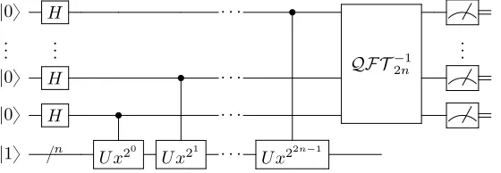
The circuit for Shor’s algorithm is as follows: since the orderr (actuallyrl{r) we are trying to

find is greater than 1, we will require multiple registers to measure it.

|0y H ¨ ¨ ¨ ‚

QF T´1 2n

..

. ... ...

|0y H ‚ ¨ ¨ ¨

|1y {n _{U x}20

U x21

¨ ¨ ¨ _{U x}22n´1

Figure 4.7: Quantum circuit for Shor’s algorithm (Wikipedia, 2017c)

[image:44.612.179.459.467.564.2]

(45)

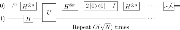
4.4.3 Grover Search

Grover’s search (Grover, 1996), formally described in Nielsen and Chuang (2002), takes a functionf such that there is at least onessuch thatfpsq “1, a setS“ t0,1unof inputs of size|S| “N “2n_,

and is able to find ansPSwhich satisfiesfpsq “1 inOp ?

Nqtime. Classically this kind of search has to take at leastN steps, and therefore takeOpNqtime. This speedup, though not exponential, is quite significant considering the generality of this algorithm. It was also proven that this is the maximal speedup possible for this problem (Zalka, 1999).

Much like ourf oracle mentioned in the Deutsch-Jozsa algorithm, letU be an oracle defined as U|xy |yy “ |xy|y‘fpxqy wherefpxq “1 ifxis a solution to the search problem and 0 otherwise. The algorithm also uses conditional phase shift which takes|0yto|0yand|xyto´ |xyforxą0. The Grover iteration used in Grover’s search is defined as a product of 4 gates. First theUgate, followed by a Hadamard gate, then conditional phase shift, and then another Hadamard gate. Together the Grover iteration looks like

G“ pHbn

p2|0ybnx0|bn´InqHbn qU

Nielsen and Chuang (2002).

To demonstrate how the Grover operator is able to give the desired answer, a geometric analysis is quite useful. LetM denote the number of solutions tofpsq “1, that isM “ |tsPS :fpsq “1u|.

Let|βy “ ?1

M

ř

x:fpxq“1|xy be the vector of all M solutions, and |αy “ 1

?

N´M

ř

x:fpxq‰1|xy,

then we can write the uniform state as

1

?

2n

2n´1

ÿ

x“0

|xy “

c

N´M N |αy `

c

M N |βy.

The oracle transform reflects |βyabout|αy; mathematically we can write this as

Uωpa|αy `b|βyq

ˆ

|0y ´ |1y ?

2

˙

“a|αy

ˆ

|0y ´ |1y ?

2

˙

`b|βy

ˆ

|1y ´ |0y ?

2

˙

“ pa|αy ´b|βyq

ˆ

|0y ´ |1y ?

2

˙

The transformpHbn

p2|0y x0| ´IqHbn

q is a reflection about ?1

2n

ř2n´1

x“0 |xy. Performing these

two reflections together gives a rotation. Let cosθ₂ “

b

N´M

N , then we have that sin θ

2 “

b

M

N and we can re-write the uniform state as,

1

?

2n

2n_´₁

ÿ

x“0

|xy “cosθ

(46)

Then applying the Grover iteration to both sides we get G ˜ 1 ? 2n

2n´1

ÿ

x“0

|xy

¸

“ pHbnp2|0ybnx0|bn´InqHbnqUω

ˆ

cosθ

2|αy `sin θ 2|βy

˙

“ pHbn

p2|0ybnx0|bn´InqHbn q

ˆ

cosθ

2|αy ´sin θ 2|βy

˙ “cos ˆ 3θ 2 ˙

|αy `sin

ˆ

3θ 2

˙

|βy

and applying the iterationktimes leads to

Gk

˜

1

?

2n

2n_´₁

ÿ

x“0

|xy

¸

“cos

ˆ

2kθ`θ 2

˙

|αy `sin

ˆ

2kθ`θ 2

˙

|βy.

Thus we perform the iteration a number of times so that sin`2kθ`θ

2

˘

is close to 1, which leads to k“ S π 4 c N M W .

This can be derived by

sin

ˆ

2kθ`θ 2

˙

«1 2kθ`θ

2 «

π 2 θ2k`1

2 «

π 2 2k`1« π

θ

k« π

2θ ´ 1 2 k« π

4 c N M ´ 1 2

We could include the`2mπin the second line, however we are trying to use the least number of iteration steps so we pickm“0 in this case. Now that we have shown how the Grover iteration is able to find the desired answer, the algorithm for producing the single uniquex1_{such that}_f

px1

(47)

|0ybn|0y Ñ ?1

2n

2n_´₁

ÿ

x“0

|xy p|0y ´ |1yq Hadamard

then repeat the Grover iterationrpπ?N{4qstimes

Ñ ppHbn

p2|0y x0| ´IqHbn qUrpπ

?

N{4qs

q

˜

1

?

2n

2n_´₁

ÿ

x“0

|xy p|0y ´ |1yq

¸

“Grpπ ?

N{4qs

˜

1

?

2n

2n´1

ÿ

x“0

|xy p|0y ´ |1yq

¸

« |βy

ˆ

|0y ´ |1y

2

˙

“ˇˇx1 D

ˆ

|0y ´ |1y

2

˙

[image:47.612.96.401.112.297.2]

Ñx1 Measurement on firstnqubits

Figure 4.8: Quantum Search Algorithm (Nielsen and Chuang, 2002)

To produce a quantum circuit, we can just write out each transform used in order. Grover operator

|0y {n Hbn

U

Hbn ₂_|₀_{y x}₀_{| ´}_I _Hbn _{¨ ¨ ¨}

|1y H ¨ ¨ ¨

RepeatOp ?

Nqtimes

Figure 4.9: Quantum Circuit for Grover’s algorithm (Nielsen and Chuang, 2002; Wikipedia, 2017a)

It may not be immediately obvious what our value ofM should be, that is, how many solutions there may be. It turns out that we can solve this problem with our next algorithm.

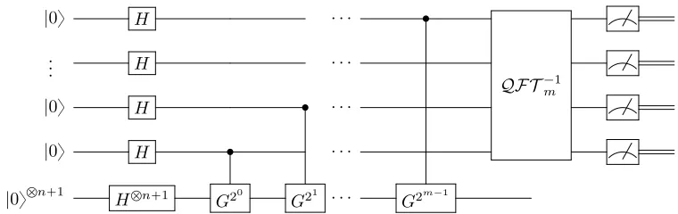
4.4.4 Quantum Counting Algorithm

The Quantum Counting Algorithm, proposed in Brassard et al. (1998) and described in Nielsen and Chuang (2002), is a combination of Grover search and phase estimation. Given an oracle indicator functionfB : AÑ t0,1uof B ĎA, with |A| “N “2n, the Quantum Counting Algorithm finds

[image:47.612.131.430.403.453.2]

(48)

To do so, the Quantum Counting Algorithm finds a solutionθ to the equation sin2 ˆ θ 2 ˙ “ M

2N (4.4)

then solves for M.

Phase estimation, described in Section 4.3.4 and Nielsen and Chuang (2002), is a subroutine used in quantum algorithms to estimate the phase of the eigenvalue of some unitary operator (in this caseG) to some precision. Phase estimation relies on the fact that when the eigenvalue is written in the forme2πijφ _{for phase}_φ_{, the inverse Fourier transform will transform} _?1

N

řN´1

j“0 e 2πijφ

|jy to an approximation of φin the form

ˇ ˇ ˇ

˜

φE, where ˜φis the binary approximation of φ.

To achievembits of accuracy ofθwith probability 1´, the algorithm works on two registers. The first register is of sizet“m`rlogp2`₂1qs, and the second register of sizen`1.

The algorithm is much like the phase estimation described in Section 4.3.4.

|0ybt|0yn`1Ñ 1

2t{2 2t_´₁

ÿ

k“0

|ky 1

2pn`1q{2 2n`1_´₁

ÿ

s“0

|sy Hadamards

Ñ 1

2t{2 2t_´₁

ÿ

k“0

e2πiφk|ky 1

2pn`1q{2 2n`1_´₁

ÿ

s“0

|sy Controlled-G

“ 1

2t{2

´

|0y `e2πi2t´1φ|1y

¯ ´

|0y `e2πi2t´2φ|1y

¯

. . .

´

|0y `e2πi20φ|1y

¯ ₁

2pn`1q{2 2n`1_´₁

ÿ

s“0

|sy

“ 1

2t{2

`

|0y `e2πi0.φt_|₁_y˘ `_|₀_{y `}_e2πi0.φt´1φt_|₁_y˘

. . .`|0y `e2πi0.φ1...φt_|₁_y˘ 1

2pn`1q{2 2n`1´1

ÿ

s“0

|sy

Ñ

ˇ ˇ ˇφ˜

E 1

2pn`1q{2 2n`1´1

ÿ

s“0

|sy Inverse Fourier transform

Ñφ˜ Measurement on first register

(49)

|0y H ¨ ¨ ¨ ‚

QF T´1

m

..

. H ¨ ¨ ¨

|0y H ‚ ¨ ¨ ¨

|0ybn`1 Hbn`1

[image:49.612.78.458.94.214.2]

G20 G21 ¨ ¨ ¨ G2m´1

Figure 4.10: Quantum Circuit for the Quantum Counting algorithm (Nielsen and Chuang, 2002; Wikipedia, 2017b)

If we choosem“rn{2s`1 andsufficiently small (such as 1{10), then the algorithm will take Op?NqGrover iterations. This means that the functionf will only be calledOp?Nqtimes. Note that this is in contrast to a classical (deterministic or probabilistic) algorithm which will takeOpNq

oracle calls to achieve the same accuracy. Formally,

Theorem 4.4.1(Quantum Counting Correctness). Given a functionf :t0,1unÑ t0,1usuch that

M “ |txP t0,1un:fpxq “1u|andsin2`θ₂˘“ ₂M_N, to findθwithmbits of accuracy, with probability

1´the Quantum Counting Algorithm requiresOpm`n`rlogp2`₂1qsqregisters andOp ?

Nqtime.

Proof. The majority of this proof is from Nielsen and Chuang (2002). Given mand set up the first register withrlogp2`₂1qsqubits, and the second register withn`1 qubits. Use the Hadamard gate on the second register to take it to the superposition of ?1

2n`1

ř2n`1_´₁

x“0 |xy. Like the Grover

search algorithm let|ay and|byrepresent the eigenvectors of the Grover iteration with eigenvalues eiθ _and_eip2π´θq_{respectively. The superposition of the second register can be written in the form of}

|ayand|by. The phase estimation algorithm 4.3.4 allows us to estimate the phase of the eigenvalues of|ayor|by, that isθor 2π´θ, to within|4θ| ď2´m_{with probability at least 1}

´. Therefore we are able to determineθto an accuracy of 2´m_{with probability at least 1}

´.

4.4.5 Harrow-Lloyd Algorithm for Linear equations

Given some NˆN matrixAand some vector b, finding the solution xto the equationAx“b is known as the linear equation problem. Classically this can be done in many ways, such as matrix inversion (finding A´1 _{such that}_x

“A´1_b_{). Classically the fastest algorithm takes}_O

pN κq time, where κis the condition number of the matrix A. The Harrow-Lloyd algorithm (Harrow et al., 2009) is able to achieve an exponential speedup in N by taking OplogpNqκ2

q time, if κ“ Op1q. Note that whenκ“OpNqthis algorithm provides no speedup.

(50)

some property of x, such as ||M x||tr for some matrix M, it will provide an exponential speedup over classical methods. The procedure relies on the quantum phase estimation and hamiltonian simulation, for both of which there are fast quantum algorithms.

4.5 Quantum Complexity Theory

Quantum complexity theory is developed in the landmark paper by Bernstein and Vazirani (1997), which expands on Deutsch’s work by defining what it means for a QTM to be well-formed. Then showed that well-formedness of a QTM is equivalent to having a unitary time evolution operator (as Quantum Physics requires). Then, it goes on to demonstrate how to (theoretically) construct an effi-cient universal QTM. This is done by proving some results about reversible Turing Machines, which in turn apply to Quantum Turing Machines, since unitary transforms are by definition reversible. Then Bernstein and Vazirani (1997) used those results to construct a looping and branching pro-cess required by an efficient QTM. To show how to decompose a unitary transform, Bernstein and Vazirani (1997) defined a class of matrices called near-trivial.

Definition 4.5.1. A near-trivial matrix is one that is the identity with either a single diagonal phase shift,eiθ, or a rotational block of the form

ˆ

cospθq ´sinpθq

sinpθq cospθq

˙

for someθP r0,2πq.

It was then proven that there exists a (deterministic) polyplogp1qq algorithm to decompose any unitary matrix into near-trivial matrices. Bernstein and Vazirani (1997) used θ “ R :“

2πř8_k_“₁2´2k

and showed that one can efficiently simulate any QTM with near-trivial transforms with this choice ofR. Quantum Turing Machines of the above form, withθ“R, are hereby referred to asQT MBV.

All of this led to the definition of the Quantum complexity classes of BQP (Bounded Error Quantum Polynomial time), an analogue ofBPP, andEQP(Exact Quantum Polynomial Time).

Definition 4.5.2. BQP is defined as the set of languages that are accepted with probability 2₃ by some polynomial time Quantum Turing Machine.

(51)

4.6 Quantum Computability

Quantum computability was expanded on by Adleman et al. (1997). Here, the authors used tran-scendental number theory and were able to produce some results about the computational power of different classes of Quantum Turing Machines. Similarly to Bernstein and Vazirani (1997), Adleman et al. (1997) defined a type of QTM much like the near-trivial QTM, i.e. one whose transforms are near-trivial matricies. LetθP r0,2πq, then letQT Mθ denote a subset of allQT M s, whose matrix

(time evolution operator) is block diagonal with each block containing 1,´1, or a 2ˆ2 of the form

ˆ

cospθq ´sinpθq

sinpθq cospθq

˙

.

LetQT M_Q“Ť_q_P_QQT Mq and letQT MBV be the Quantum Turing Machine defined by Bernstein

and Vazirani (1997). Adleman et al. (1997) showed thatQT M_Q”QT MBV in the sense that they

can simulate each other within some small ą 0 error, with only a polynomial slowdown. Let BQPθ denote BQPas defined above for QT Mθ. Adleman et al. (1997) proved that this leads to BQP “ BQP_Q. However, they were also able to prove that BQP_Q Ĺ BQP_C, and that BQP_C contains sets of arbitrary Turing degrees. Recall that Turing degrees (Post, 1944) are the degree of difficulty of a problem, that is, how unsolvable a problem is. This then leads to the fact thatQT M_Q cannot simulate QT M_Cwitherror in polynomial time. Additionally, Adleman et al. (1997) were able to prove that BQP and EQP are all contained within PP. Recall that PP (Probabilistic polynomial time) is the class of all problems solvable with a probabilistic Turing Machine which is correct with probability more than 1₂ (Gill, 1977). If we defineEQPθ similar toBQPθ, then forθ

such that cospθqis poly-computable transcendental,EQPθ“P.

4.7 Quantum Algorithmic Information Theory

Little work has been done on Quantum Algorithmic Information Theory compared to other areas of Quantum Computing. Quantum Kolmogorov complexity was first discussed by Berthiaume et al. (2000). M¨uller (2008) expanded upon the idea, and defined it as follows,

Definition 4.7.1 (M¨uller (2008)). Given a QTM M and a finite error δ ą 0, the finite-error Quantum Kolmogorov complexity of a qubit string|xy is

K_M,δQ pxq “min

p t`ppq : ||x´Mppq||trăδu

and the approximate-scheme Quantum Kolmogorov complexity of a qubit string xis

K_MQpxq “min

p

"

`ppq : ||x´Mpp, kq||tră 1

k @ kPN

*

where|| ¨ ||tr is the trace norm, i.e. ||a´b||tr:“ 1₂||a´b||1.

(52)

satisfies the property that for any other QTMM we have K_UQpxq ďK_MQpxq `cM

for all qubit strings x, where cM is a constant depending only onM, but not on x. Then M¨uller

(2008) goes on to prove that for allδ, γPQ` withδăγ, and for all QTMM we have that K_UQ_,γpxq ďK_M,δQ pxq `cM,γ,δ

for all qubit strings x, where cM,γ,δ is a constant depending on M, γ and δ. This shows that the

Quantum Algorithms for Universal Prediction