1973
Theory of some free surface groundwater seepage
problems
Muhammad Yunus Khan
Iowa State University
Follow this and additional works at:https://lib.dr.iastate.edu/rtd Part of theHydrology Commons
This Dissertation is brought to you for free and open access by the Iowa State University Capstones, Theses and Dissertations at Iowa State University Digital Repository. It has been accepted for inclusion in Retrospective Theses and Dissertations by an authorized administrator of Iowa State University Digital Repository. For more information, please contactdigirep@iastate.edu.
Recommended Citation
Khan, Muhammad Yunus, "Theory of some free surface groundwater seepage problems " (1973).Retrospective Theses and Dissertations. 4948.
INFORMATION TO USERS
This material was produced from a microfilm copy of the original document. While the most advanced technological means to photograph and reproduce this document have been used, the quality is heavily dependent upon the quality of the original submitted.
The following explanation of techniques is provided to help you understand markings or patterns which may appear on this reproduction.
1. The sign or "target" for pages apparently lacking from the document photographed is "Missing Page(s)". If it was possible to obtain the missing page(s) or section, they are spliced into the film along with adjacent pages. This may have necessitated cutting thru an image and duplicating adjacent pages to insure you complete continuity.
2. When an image on the film is obliterated with a large round black mark, it is an indication that the photographer suspected that the copy may have moved during exposure and thus cause a blurred image. You will find a good image of the page in the adjacent frame.
3. When a map, drawing or chart, etc., was part of the material being photographed the photographer followed a definite method in "sectioning" the material, it is customary to begin photoing at the upper left hand corner of a large sheet and to continue photoing from left to right in equal sections with a small overlap. If necessary, sectioning is continued again — beginning below the first row and continuing on until complete.
4. The majority of users indicate that the textual content is of greatest value, however, a somewhat higher quality reproduction could be made from "photographs" if essential to the understanding of the dissertation. Silver prints of "photographs" may be ordered at additional charge by writing the Order Department, giving the catalog number, title, author and specific pages you wish reproduced.
5. PLEASE NOTE: Some pages may have indistinct print. Filmed as received.
Xerox University Microfilms
THEORY OF SCME FREE SURFACE GROUND'WATER SEEPAGE PROBL0ÎS.
Iowa State Ifeiversity, Ph.D., 1973 Ifydrology
University Microfilms, A XEROX Company, Ann Arbor. Michigan
Theory of some free surface groundwater seepage problems
by
Muhammad Yunus Khan
A Dissertation Submitted to the
Graduate Faculty in Partial Fulfillment of
The Requirements for the Degree of
DOCTOR OF PHILOSOPHY
Departments: Water Resources Civil Engineering Majors: Water Resources
Soil Engineering
Approved :
ofMaJop
In Charge of Major Work
For the Majo Departments
For the Graduate College
Iowa State University Ames, Iowa
1973
Signature was redacted for privacy.
Signature was redacted for privacy.
TABLE OP CONTENTS
Page
INTRODUCTION AND LITERATURE REVIEW 1
UNCONPINED PLOW BETWEEN TWO PARALLEL DITCHES 12
Theoretical Analysis 12
Results and Discussion 31
TWO-DIMENSIONAL GROUNDWATER MOUNDS 62
Theoretical Analysis 62
Results and Discussion 72
THREE-DIMENSIONAL GROUNDWATER MOUNDS 8l
Theoretical Analysis 8l
Results and Discussion 92
LITERATURE CITED 101
ACKNOWLEDGEMENTS 107
APPENDIX A 108
APPENDIX B 114
APPENDIX C 121
APPENDIX D 146
1
INTRODUCTION AND LITERATURE REVIEW
Water, being a vital part of our environment, has
attracted the attention of scientists during recent years.
Groundwater, because it is often fresh and hence suitable for
human and plant use has attracted particularly great attention.
Briggs and Fiedler (1966, p. 5) have estimated that, at any
moment, 97 percent of fresh water supply of the world, is
found below ground, an amount equal to about 8 trillion acre
feet. When this fact is considered along with the increased
emphasis on the preservation of natural resources, it becomes
imperative that the mechanism of groundwater flow should be
understood completely. An understanding of flow of groundwater
has applications in such areas as drainage of farm land, sta
bility of dams, analysis of land slides, and prediction of water
table near ditches and wells.
In groundwater hydrology, the term aquifer refers to any
porous medium that is permeable enough to store and yield
water in useful quantities. An aquifer may be confined or
un-confined. A confined aquifer is bounded on top and bottom by
impermeable strata. An unconfined aquifer, on the other hand,
has no overlying Impermeable stratum and is characterized by a
water table also known as free surface. A free surface is an
air-water interface that forms the top boundary of the flow
domain and is always under atmospheric pressure. In most
unconfined systems the free surface outcrops above the
The theory of unconfined flow is not as well developed
as of confined flow primarily because of its complexity.
Factors responsible for this complexity are the unknown shape
of the free surface a priori and the occurrence of surface
of seepage in most unconfined systems. The length of the
surface of seepage is also not known initially because its
upper terminal always joins with the free surface.
The presence of a surface of seepage has been proven
mathematically by Davison (1936) and explained through logical
reasoning by Muskat (1946). The phenomenon of a surface of
seepage occurs in both steady and unsteady unconfined flow
conditions. It is least understood and is most often neglected,
by making simplifying assumptions. However, its importance
should not be underestimated. Wenzel (1942) and Ineson (1952,
1953) demonstrated the usefulness of determining the exact
shape and location of the free surface. For example, measure
ments made close to the well during a field pumping test can,
without a consideration of the surface of seepage, lead to seri
ous errors in the values of aquifer constants - hydraulic con
ductivity and storage coefficient. Some of the common mathe
matical approaches which neglect the effect of surface of seepage
in the analysis of unconfined flow are discussed here.
The easiest approach is the adaptation of the theory of
confined flow to analyze the problems of unconfined flow.
3
flowlines in unconfined flow systems. This is also known as
horizontal flow analysis. The basic assumptions Involved in
this approach are:
(1) The impermeable barrier underlying the aquifer
is horizontal.
(2) Flow velocities are parallel with the impermeable
barrier.
(3) The depth of flow remains essentially constant. In
other words, the resulting drawdown of the free sur
face is small.
The Just-mentioned assumptions make the unconfined flow
analogous to conduction of heat in solids. Consequently, a
vast number of published solutions available in the field of
heat conduction have been used advantageously for.unconfined
flow. Carslaw and Jaeger (1959) give numerous solutions for
heat conduction problems. An example of the application of
the horizontal flow analysis is the use of Theis (1935)
non-equilibrium equation to solve the problem of unsteady uncon
fined flow toward a well. Maasland and Bittinger (1963) give
an excellent review of solutions of this category for both
two-dimensional and axisymmetric unconfined flow systems. For
some flow situations this simplified approach may yield satis
factory solutions for the unconfined flow.
A second mathematical approach that ignores the
presence of surface of seepage is based on Dupuit-Forchheimer
essentially constant in the horizontal flow analysis is now
considered variable in the D.F. analysis. For the
steady-state unconfined flow, the Dupult-Porchheimer assumptions yield,
a simple equation that leads to the well-known Dupuit curve.
For the unsteady unconfined flow, however, the D.F. equation
becomes nonlinear and is difficult to solve.
Polubarinova-Kochina (1962) gives two methods of linearizing the D.F.
equation for a two-dimensional unconfined flow system.
Haushlld and Kruse (I960) present an interative linearizing
method. It can, however, be proved that the result is the
same as that obtained by using the linearized equation of
Polubarinova-Kochina. Glover and Bittinger (1961) extend the
interative linearizing scheme of Haushlld and Kruse to
axi-symmetric flow toward a well. Recently, Karadl, e^ aJ. (1968),
Yeh (1970) and Hornberger, et aJ^. (1970) present different
numerical techniques to solve the D.F. equation for the
two-dimensional unconfined flow while Kriz, e^ al. (1966) and
Monkmeyer and Murray (1968) solve the Dupuit-Forchheimer equation
for axisymmetric unconfined flow toward a well, also by using
a numerical technique.
Dupuit-Forchheimer theory has been criticized severely
by Muskat (1946) and Kirkham (1967) and its validity and limita
tions have been discussed by Hantush (1963), Bouwer (1965),
Glover ( 1 9 6 5 ) , ^an Schllfgaarde (1965), and DeWlest (1965).
5
of the ease of its application and because it is a good first
approximation to more rigorous solutions for many flow situa
tions .
A third approach that neglects the presence of surface
of seepage is based on solving Laplace's equation by linearized
boundary condition of the free surface. In this analysis,
vertical velocities that have been neglected in all the litera
ture discussed previously are taken into account. Boulton
(1954) and Streltsova and Rushton (1973) use this type of
linearizing technique to solve a problem of unsteady,
uncon-fined groundwater flow toward a well. Dagan (1964) and
DeWiest (1962) extend this linearizing technique by using
perturbation.
In the previously mentioned literature the existence of
the surface of seepage was neglected. The first approximate
method that accounts for the development of the surface of
seepage was proposed independently by Schaffernak (1917) and
van Iterson (1917). Both writers propose the same method which
deals with steady-state unconfined flow through an earth dam
founded on a horizontal impervious base. The method is simple
and the solution lends itself to a simple graphical construc
tion for the determination of the surface of seepage.
Casagrande (1932) analyzes and improves the same problem of
seepage through an earth dam by taking the hydraulic gradient
as dy/ds instead of dy/dx. Here s is the distance measured
of Casagrande's solution. Pavlovsky (1931) also gives a
solution of the same problem. He divides the flow region of
the earth dam into three zones-and assumes horizontal flow in
the two outer zones and the Dupuit-Forchheimer type flow in
the middle zone. His analysis results in two equations (with
two unknown) which' can be solved without difficulty to deter
mine the surface of seepage.
In the analysis of unsteady unconfined flow situations,
generally an estimated or experimentally measured length of
surface of seepage is added, a posteriori, to the solution
which normally neglects its effect. Mahdaviani (196?) uses
an estimated length of surface of seepage in analyzing unsteady
flow toward gravity wells, while Chauhan, et al. (1968) use an
experimentally measured length in an unsteady two-dimensional
tile drainage problem.
Muskat (1946) and Polubarinova-Kochina (1962) present
exact analyses of steady-state unconfined flow through an
earth dam. Their analyses are based on the velocity hodograph
technique. To introduce the velocity hodograph, let the
complex potential w = (p + lijj be an analytic function of the
complex variable, z, as w = f(z). Differentiating w with
respect to 2, we find
dz 9x 9x
which, on substitution of the horizontal and vertical compo
7
velocity
^ = i l
= ^
The transformation of the region of flow from the z plane
into the W plane is called, the velocity hodograph. The
utility of the hodograph stems from the facts that, although
the shape of the free surface and the limit of the surface of
seepage are not known a priori in the z plane, their hodographs
are completely defined in the W plane. It has been proved by
Huskat and Poluborinova-Kochina that the free surface boundary
of a flow region is transformed to a circle into a W plane.
This circle passes through the origin, with radius k/2 and
center at (0, -k/2). Here k is the hydraulic conductivity of
the flow region. The surface of seepage and impervious bound
ary are transformed to straight lines into the W plane. The
mathematical analysis of the velocity hodograph is tedious.
Moreover, the technique does not lend itself to the construc
tion of a flow net.
There are several numerical methods for solving exact
partial differential equations of groundwater flow. Of these,
only one stands out as being universally applicable to both
linear and non-linear problems - the method of finite differ
ences. Charmonman (I965) presents a simple method of deter
mining the free surface of a steady-state two-dimensional
un-confined flow by solving Laplace's equation in the
tion is based on relaxation method and lends itself to
easy-computation of flow nets. His method or the hodograph method,
however, cannot be extended to axisymmetric flow situations.
Boreli (1955), Shaw and Southwell (1941), Taylor and
Brown (1967), Finn (1967), and Finnemore and Perry (1968)
also use different finite element methods to solve
steady-state two-dimensional and axisymraetrlc flow problems exactly.
Kashef (1965a, 1965b) gives solutions of both the unconfined
seepage through earth dams and unconfined flow toward a
gravity well. His solutions are based on analyzing the
hydrodynamic forces within the flow region.
Kirkham (1964), by solving simultaneous equations and using
a simple iterative scheme, found a supposedly exact analysis for
both two-dimensional flow through a dam and axisymmetric flow
toward a well. His method was based on collocation, i.e.,
solving equations for a number of points on the free surface.
However, his analysis breaks down when more than about 6 points
are considered on the free surface. Murray (1970) points out a
flaw in Kirkham's analysis and arrives at a modified solution
by using spline functions. It is, however, doubtful to say if
Murray's method can be generalized because his selection of
the location of points, which are very critical for the proper
steady-state solution, is based on trial and error method
(see his p. 44 and appendix B). No criterion is given for the
selection of the location of points. Murray does not carry
9
Perhaps the most significant recent literature in the
theoretical analysis of unconfined flow is by Taylor and
Luthin (1969)5 Dicker (1969), Yerma and Brutsaert (1970) and
Todsen (1971). Taylor and Luthin present a method for using
numerical analysis and a digital computer to solve problems
of free surface around a pumped well in an unconfined aquifer.
Their method takes into account the properties of the unsatu
rated portion of the aquifer and can be adapted to a variety
of water flow problems. Dicker, by drawing an analogy between
the velocities of flow across the surface of seepage and an
orifice flow, postulates a new set of boundary conditions and
develops a new theoretical solution very much different from
the "exact" solution based on potential theory. His solution,
however, has not been tested experimentally so far.
Another important free surface problem is the development
of groundwater mounds in water spreading for artificial recharge
or waste disposal. Farvolden and Hughes (1969) discuss sani
tary landfill design criteria to minimize pollution of ground
and surface water. The generation and movement of contaminants
in a sanitary landfill depend upon the content, spatial distri
bution, and time variation of moisture within that landfill.
The best way to minimize water contamination is to keep the
landfill unsaturated so that aerobic decomposition of organic
material and rapid drainage can take place. When the fill must
must be selected to prevent fast migration of leachate, or to
provide convergent flow toward collection sites. Therefore,
knowledge of the occurrence and movement of moisture within
a sanitary landfill and in the groundwater mound that develops
under the fill is basic to a knowledge of the generation and
movement of waterborne contaminants. Remson e^ a2. (1968)
suggest a moisture-routing method to determine the moisture
regimen of a sanitary landfill. Most recently Bouwer ejb al.
(1972) have used infiltration basins to renovate secondary
sewage. The prediction of position of the water table during
and after water infiltration is of considerable operational
importance. Basin geometry and spacing, as well as the period
of water spreading are the operational controls that can be
used to prevent the rise of the water table.
Baumann (1952) initiated the study of formation of ground
water mounds. Later on^ Glover (I96I), Bittinger and Trelease
(1965)5 Hantush (1967), Bianchi and Haskell (1966, 1968), and
Haskell and Bianchi (1965) contributed to the theory of
groundwater mounds. However, all these theoretical develop
ments are approximate, being based on Dupuit-Forchheimer
assumptions. Bouwer (1962), however, has developed an analog
model of analyzing groundwater mounds by a resistance network.
In this thesis, analytical methods have been developed
from potential theory for determining heights of the free surface
11
(1) two-dimensional seepage between two parallel ditches
when water level in one ditch is higher than the
other. This flow situation is also termed as flow
through a vertical dam.
(2) flow in a two-dimensional groundwater mound formed
by percolation of recharge water from a rectangular
basin, and
(3) flow in a three-dimensional groundwater mound formed
by percolation of recharge water from a circular
basin.
The methods are based on solving appropriate differential equa
tions and applying an iterative scheme. Plownets have been
prepared for all 3 problems to help in understanding the physics
of flow. Tables of heights of free surface have been prepared
for use in the field. An example is given to illustrate the
UNCONFINED FLOW BETWEEN TWO PARALLEL DITCHES
A simplified model of an unconfined, steady-state,
two-dimensional groundwater flow is shown in Pig. 1. Two
parallel ditches penetrate down to a horizontal impermeable
base OA. The water stands at heights h^ and h^, respectively,
in the right and the left ditches. Water, seeping through the
aquifer, outcrops at C, forming DC the line of seepage face.
The aquifer is not confined by any top impervious layer; a
water table forms the top boundary of the flow domain. Such
a flow system with a ponded water was analyzed by Kirkham
(1965). The analysis of the ponded water flow situation,
however, does not involve a seepage face or a free surface and
is therefore relatively simple.
Theoretical Analysis
In the formulation of our mathematical model, the aquifer
is assumed homogeneous and isotropic and capillary effects are
neglected. We choose an origin 0 of (x,y) coordinates at the
left bottom corner of the flow region, shown in Fig. 1, and
the impermeable base as the datum for determination of hydraulic
potential which is measured positive in the vertically upward
direction. We denote hydraulic potential and stream function
at any point (x,y) by *(x,y) and i|;(x,y), respectively. The
potential #(x,y) is related to gauge pressure p' and height y
above the datum by
Figure 1. A simplified model of an unconfined flow between
ground surface
free surface
y.axis
P(X:,h. )x-axis
/ / / / / / / / ) / / ) / / / / J / / / f / / / / / / / f / / f / / / / f / / f / / / / / / /
0
impermeable base
A
15
where y is the density of water (mass per unit volume). When
Darcy's law, which governs the motion of groundwater, is com
bined with the equation of continuity, a partial differential
equation results. For a steady-state flow, the partial
differential equation becomes Laplace's equation which, in a
two-dimensional coordinate system (x,y) is written as
.2. ^2. 3'
I- + M = 0 [2]
3x^ 3y^
Potential and stream functions
The problem is to develop analytical expressions for
*(x,y) and '|'(x,y) such that they satisfy equation [2] as well
as the following boundary conditions (EC's):
Along OA Tp = 0 or 3<J)/3y = 0 BC 1
Along AB <j) = hg BC 2
Along BC (t> = h(x) BC 3
ij; = q BC 4
Along CD <f> - y BC 5
Along OD <j> = h^ BC 6
where q, in BC 4, is the discharge per unit width of the flow
to give an exact formula for q (Hantush, 1963). For a
constant hydraulic conductivity k, the expression for q is
From the general solution of equation [2], given by
Kirkham and Powers (1972, p. 57), we can now develop a partic
ular solution to satisfy our boundary conditions. We define
*m Bp by
= m ir/L [4]
and
3 = (2p - 1) n/2h
[ 5 1
P ^
so that, in view of boundary conditions 1 and 2 and in antici
pation of using Fourier series expansion to satisfy EC's
5, 6, and 7, the «|>(x,y) is written as
h x(h - h ) " sinh 3 (L - x)
^ = 4' - p!i 'p'
00 cosh a y
+ : \ cosh V 1^" m=l m e
where A and are dimensionless but arbitrary constants. m p
17
and superscript ™ from the summation signs.
We can write an expression for the ^(x,y) by using
Cauchy-Riemann relations but Kirkham and Powers (1972, p. 106) give
a handy table which is used here to develop ^^x,y) as
ih (K - h )y cosh 3 (L - x)
IcE- = L h + : Bp slnh^ L 6 y
e e p ^
sinh a y
+ ^ % cosh A V
m e
Equations [6] and [7] satisfy EC's 1 and 2, irrespective
of any values of and In order to satisfy EC's 5, 6,
and 7 we put x = 0 in equation [6] and obtain
= ^ - Z B cos B y [8]
e e
which is a quarter-range cosine series. EC's 5, 6, and 1 will
be satisfied if the are
Kirkham (196$, eq. 24), as
be satisfied if the are chosen, by using the method of
e e Q c
which, upon substitution for 0(0,y) and subsequent integration,
yields the as
8[cos(3 h /h ) - cos(3 h /h )]
B = P ^ ^ 5 ^ — [9]
Free surface boundary conditions
All the boundary conditions of the real flow region except
that at the free surface are now satisfied. We have developed
two different methods of satisfying the free surface boundary
conditions. They are:
(i) by forming a set of N simultaneous linear equations
by the use of an artifice and then solving the result
ing simultaneous equations to determine of equation
[6] and [7]. Hereafter we shall refer to this as the
simultaneous equation method.
(ii) by using a technique known as the modified
Gram-Schmidt orthonormalization technique to solve a set
of non-linear equations to determine A^ of equations
[6] and [?]• The method has been developed by Powers,
et al. (1967) and explained in detail by Kirkham and
Powers (1972). Hereafter this method will be called
the PKS method.
The simultaneous equations method Instead of consider
ing only the boundary conditions of the real flow region, OABCD
in Fig. 1, we consider a composite rectangular flow region OABE
in which BCE is a fictitious potential flow region of hydraulic
conductivity k. The flow in this fictitious region results from
water being introduced along BE. This water is added to make
BC a streamline and simultaneously a free surface. Kirkham
19a
restrictive. Murray (1970) points out this flaw and assumes
a curvilinear potential distribution along CE. In this
analysis we take a constant potential h^ along this boundary.
This simple potential distribution will simplify the analysis
considerably. The potential distributions of Kirkham, of
Murray, and the distribution we shall find in this analysis
are compared in Pig. 2. The potential distribution along BE
is not assumed; it is left to adjust itself to satisfy the
boundary conditions along the free surface. The point E,
however, is under suction (potential h^ being less than the
gravity head h^). Therefore, we anticipate that boundary BE
will be under suction except at point B where p' = 0. We now
can write the extra boundary conditions for the fictitious
region.
Along CE $ = hg (= constant) BC 7
Along EB <j) = f(x) BC 8
where f(x) is yet to be determined. To insure continuity we
must keep f(0) = h^ and f(L) = h^. We express f(x) as
. . h x(h -h ) N
—i"— = ii— + —f—c + Z a C O S [ (2n—1 )Trx/2L] [10]
e ^ ^e n=l,2,... ^
where N, as will be explained later, depends upon the number of
19c
... Murray's potential distribution
— Kirkham's potential distribution
Equation [10] is a quarter-range cosine series. Other
series (sine and power series) we have tried complicate the
analysis and are not reported.
We have explicitly required continuity of the potential,
ij) = h(x)j along the interface of the real and fictitious regions
and have also implicitly required continuity of the normal
derivative of (p at the interface. Therefore, the two regions
may be considered as one.
In view of BC 8 of the fictitious flow region we put
y = hg in equation [6] and equate the resulting expression to
the right side of equation [10]. After cancelling some common
terms we obtain
N
E A sin a X = Z a cos[(2n-l)nx/2L] [11]
^ n=l ^
Notice that sine and cosine terms of equation [11] are
identically zero at x = L. In other words, any values of A^
and a^ will satisfy equation [11] at x = L. Hence, we should
not use the point x = L in our simultaneous equations. The
A of the infinite sine series of equation [11] can be easily m
obtained from Fourier theory as
P L N
A = T / Z cos[(2n-l)x/2L] sin a^x dx
m L -, n m
0
which, upon substitution for and subsequent integration,
21
N 2 a m
A = — Z p P [12]
n=lj2,... 7T[m - (2n-l) /4]
So far we have not utilized EC's 3 and 4 of the free
surface. We shall use these conditions now to evaluate a^ and
subsequently A^. We put $ = hu in equation [6], jp = q in
equation [7], and y = h^ and x = in equation [6] and [?]
to obtain the following two equations for the free surface
...
e e e ^ p
cosh a h.
+ ^ oosh cV Vl "3]
m e
and
(h -h )h cosh 6
khg " L hg ^ ®p sinh g^L ^p^i
sinh a h.
+ Z Am cosh V±
m e
Equation [14], upon substitution of the right side of equation
[12] for A^ and rearrangement, yields
N GO 2m sinh a h. cos a x.
Z a r Î V 2^—]
n=l m=l TT{m - (2n-l) /4} cosh a^h^
The must now be chosen in such a manner that equations
[13] and [15] are simultaneously satisfied. We accomplish
this as follows.
First we condense equation [15] by defining and
by
2m sinh a h. cos a x.
r = Z 2 SLi [16]
n[m - (2n-l) /4] cosh
(h -h )h. cosh 3 (L-x.)
= t n l - ^ + Z Bp slnhgpL Bphi
so that equation [15] may be written as
nL....
Equation [18] is the key equation which yields, when
applied to N points on an assumed free surface, a set of N
linear equations which can be solved easily for a^. For
instance, a set of such equations for N = 3 (see Fig. 3) are
^1®11 ^2®21 ^3®31 " ^i
^1®12 &2&22 &3S32 = ^2 [19]
^1^13 ^2®23 ^3^33 ^ ^3
These equations can be easily solved by Gauss's elimination
<
L
>
«x,->
25
addition to others, to determine the free surface is now
described.
(1) An estimate is made, as a first approximation,
of the hg by using charts of Polubarinova-Kochina
(1962, p. 221) or by using the approximate formula
hj = - h/)/L + h„ [20]
(2) Values of x^ (i = 1,2,3,...N) of points on the free
surface are chosen. These x^ may or may not be
evenly distributed. However, they should not be too
close to the seepage face initially. In third or
subsequent iterations they may be close to the seepage
face. We choose x^ = 0.2L, x^ = 0.24L, x^ = 0.28L,
... XgQ = O. 9 6 L . x^ = 0 or x^ = L should not be
included because at these points equation [13] becomes
independent of the a_ and
n m
(3) A parabola is fitted between the points (0,hg) and
(L,hg) to yield first approximations of h^, h^, ...
as
, , , X 1/2
hi = + (hg - ^3 ) ji] [21]
(4) Using the estimated value of the h^ and the given
h^. Bp are computed from equation [9].
(5) The g^^ and f^ (n = 1,2,...,N and i = 1,2,...,N)
are now computed by substituting h^ and (computed
in steps 3 and 4) in equations [16] and [17]. These
yield a set of N linear equations which are easily
solved simultaneously to yield a first approximation
of a^j a^, ...J a^. These a^ are then put in equation
[12] to obtain a first approximation of (m =
1,2,3,..., =).
(6) To obtain a second approximation of h^, the values of
Bp, x^ and first approximation of h^ and A^ are
substituted in equation [13]. Steps 4, 5, and 6 are
repeated till the h^ settle down. Generally four or
five repetitions are sufficient.
(7) At this stage an improved value, over that of equa
tion [20], is computed. To compute h , we put x. = 0,
y = h and use the last computed values of the A in
" s m
equation [14] and then solve the resulting equation
for the hg, the only unknown. If the difference
between the h used to compute the B and the computed
s p
hg is significant, steps 4, 5, 6, and 7 are repeated
till the difference becomes negligible.
The PKS method We apply BC's 3 and 4 to equations [6]
and [7], respectively, and rearrange the resulting expressions
to obtain
h . h x . ( h - h ) s i n h g ( L - x ) i r = i r + L h - ^ ^ s l n h ^ L
e e e ^ p
cosh a h
+ " cosh Vl "2]
27
and
h ^ (h -h )h cosh g (L - x.)
2ïrh ni ^ Bp slnh g L •
e e ^ p
slnh a h
= : ^ cosh C h Vl [23]
m e
To condense equation [23] we define
cosh B (L-x.)
- ^ ®p Slnh SpL Sphl [24]
slnh a h.
' cosh c %''l [25]
m e
so that equation [23] may be written as
P(x.) = Z U^(x.) [26]
To use the PKS method equation [26] is rewritten with
double subscripts on the A's and with F(x^) changed to F^(x^)
as
^#(*1) ^ 5 ^ ^ 1, 2 , . . . [27]
Here P^(x^) denotes the N-th approximation of P(x^) and
denotes the value of in the N-th approximation. For each
value of integer N, we find a set of constants A^^ (m =
1,2,...,N) such that as we take successively larger values
for N, the sets A^^ make the corresponding approximations of
Fj^(Xi) of equation [27] more closely equal to F(x^) of equation
[26] for all values of x^.
To calculate a set of A^^, recursion relations of Kirkham
and Powers (1972, Appendix 2) are used. The relations are
N-1
and
where we have the further recursion relations
m-1 J,
mn c c J mr rn' ,
m-1 G. w
m
m-1 p D = U - Z c D
29
^mn ~ "^nr^mr ^
and we further have
w = / P(x.) U (x) dx. [28]
m Q JL XIX
"mm = ^
To compute values of (n = 1 , 2 , . . . ) , Boast ( 1 9 6 9 ) has
prepared a computer subroutine. To use his subroutine, the
sets w and U m mn are supplied by the user. We have used Boast's i-jr- ^
subroutine to compute the of equation [27]. The required
w and U were evaluated by numerical integration,
m mn °
The values of A^^ as determined from equation [27] by
the PKS method satisfy BC 8 but not BC 7. To satisfy BC 7
simultaneously an iterative technique is used. The technique
which is similar to the one used in the simultaneous equations
method is:
(1) An estimate is made, as a first approximation, of
the height h^ as in simultaneous equations method,
equation [20].
(2) The interval between x = O.IL and x = L is divided
into 90 equal parts. That is, x^ = O.IOL, x^ =
(3) A parabola is fitted between the points (0,h^) and
(L,hg) and first approximation of h^ (i = 1,2,...91)
are computed from equation [2]].
(4) Using the estimated value of the h^ and the given h^.
Bp are computed from equation [$].
(5) Now we put the earlier computed values of the x., h.
i X
(i = 1,2,...91), and Bp in equations [24] and [25].
The resulting values of the U^(x^) and P(x^) are then
used in numerical integration of equations [28] and
[29] to yield values of w^ and which when fed to
Boast's subroutine, gives the set of A^^y
(6) These A^^ and previously computed h^ and x^ are then
substituted in equation [22] to obtain a second
approximation of the h^. Steps 4, 5 and 6 are repeated
till h^ (i = 1,2,...91) settle down. Generally 4 or 5
repetitions are enough.
(7) At this stage an improvement in the value of h^ is
made. To compute the new value of h^, we put x = 0,
y = hg, and use the last computed A^^ in equation [23]
and solve the resulting equation for h^. If the
difference between h used to compute the B and the
s p
computed h^ is significant, steps 4, 5, 6, and 7 are
31
Case of no seepage face
For large L/h^ and h^/h^, the seepage face is negligible
(see Polubarinova-Kochlna, 1962, p. 221). When the seepage
face is negligible, the of equations [6] and [7] all vanish
and the determination, of the free surface is considerably
simplified. The value of h^, which is estimated initially
when the seepage face is not negligible, is fixed and now
known. Also, when the seepage face is negligible, the are
located at equally-spaced intervals along 0 _< x < L instead of
along 0. IL _< X < L.
Results and Discussion
Free surface
Both, the simultaneous equation method and the PKS method
may be used to determine the free surface with or without a
seepage face for an unconfined flow between the two parallel
ditches of Fig. 1 when L/h^ > 1. These methods do not work
for L/hg _< 1. Both methods are considered simpler than the
hodograph method or Murray's method based on spline functions.
In our methods, unlike Murray's method, the x^ (i = 1,2,...,N)
are located at equally spaced intervals along O.IL <_ x < L.
For the region 0 < x < O.IL, and when we have a seepage
face, we have not discovered a computing program that yields
reasonable results. However, because we know the values of
hg for X = 0, O.IL, 0.2L,..., l.OL we have a smooth curve for
the whole free surface. When there is no seepage face we do
¥e have developed computer programs (see appendix C)
to determine the free surface, by the simultaneous equations
method and by the PKS method, for the flow situations when
the seepage face is negligible.
In order to check our results with those of Murray we
have computed the free surface for h^/L = 0.2875, h^/h^ =
0.6 (no seepage face); and h^/L = 0.2875, h^/h^ = 0 (with
seepage face), the parameters used by
Murray-The cost of computation of a free surface for a partic
ular geometry given in this dissertation never exceeded
$4.00, when there was no seepage face (CD = 0 in Fig. 1).
When there was a seepage face (CD ^ 0 of Pig. 1), the maximum
cost of computation of a seepage face did not exceed $12.00.
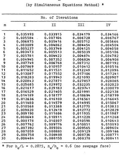
Case of no seepage face Table 1 gives values of the
(m = 1,2,...30) at successive iterations of the simultaneous
equations method. It is seen that, in 4 iterations, the
have stabilized fairly well. For better values of the A^,
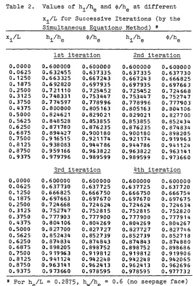
more iterations are needed. However, Table 2, which compares
values of the h^/h^ and <j)(x^,h^)/h^ for different values of
x^. at successive iterations, shows that h^/h^ and <}>(x^,h^. )/h^
are essentially equal after the fourth iteration and further
iterations were unnecessary.
Fig. 4 gives a curve of the height of the free surface
prepared from Table 2, iteration 4. Points from the free
33
Table 1. Values of the A for Successive Iterations m
(by Simultaneous Equations Method) *
No. of Iterations
m I II III IV
1 0.035993 0. 033915 0.034179 0 .034166 2 0.005584 0. 007106 0.006728 0 .006767 3 0.006875 0. 005416 0,005712 0 .005666
H 0.003089 0. 004862 0.004454 0 .004504 5 0.005237 0. 003749 0,004125 0 .004058 6 0.003473 0. 005513 0,005039 0 .005106 7 0.005781 0. 004422 0.004874 0 .004782 8 0.004945 0. 007352 0 .006824 0 .006908 9 0.007749 0. 006768 0.007312 0 .007192 10 0.007869 0. 010957 0.010412 0 .010516 11 0.011652 0. 011531 0.012249 0 .012096
12 0.013087 0. 017552 0.017106 0 .017241
13 0.018283 0. 019943 0.021093 0 .020907 14 0.020843 0. 027871 0.027857 0 .028065 15 0.025685 0. 029972 0.032235 0 .032023 16 0.021617 0. 029183 0.029741 0 .030079 17 0.016529 0. 021405 0.021991 0 .022138 18 0.014189 0. 018177 0.018694 0 .018799 19 0.012636 0. 016100 0.016561 0 .016645 20 0.011480 0. 014579 0.014995 0 .015067 21 0.010568 0. 013388 0.013770 0 .013833 22 0.009820 0. 012419 0.012772 0 .012829 23 0.009190 0. 011606 0.011935 0 .011987 24 0.008649 0. 010911 0.011220 0 .011268 25 0.008178 0. 010307 0.010598 0 .010643 26 0.007762 0. 009776 0.010051 0 .010093 27 0.007392 0. 009304 0.009565 0 . 009604 28 0.007059 0. 008880 0.009129 0 .009166 29 0.006758 0. 008498 0.008736 0 .008771 30 0.006484 0. 008150 0.008378 0 .008411
[image:40.594.118.507.109.615.2]Table 2. Values of and at different
x^/L for Successive Iterations (by the
Simultaneous Equations Method) *
x^/L hl/^e O/h, 0/h,
1st iteration 2nd iteration
0. 0000 0. 600000 0. 600000 0. 600000 0. 600000 0. 0625 0. 632455 0. 637335 0. 637335 0. 637730 0. 1250 0. 663325 0. 667243 0, 667243 0. 666825 0. 1875 0. 6 92820 0. 697935 0. 697935 0. 697663 0. 2500 0. 721110 0. 725452 0. 725452 0. 724668 0. 3125 0. 748331 0. 753447 0. 753447 0. 752747 0. 3750 0. 774597 0. 778996 0. 778996 0. 777903 0. 4375 0. 800000 0. 805163 0. 805163 0. 804106 0. 5000 0. 824621 0. 829021 0. 829021 0. 827700 0. 5625 0. 848528 0. 853855 0. 853855 0. 852434 0. 6250 0. 871780 0. 876235 0. 876235 0. 874834 0. 6875 0. 894427 0. 900180 0. 900180 0. 898205 0. 7500 0. 916515 0. 921174 0. 921174 0. 919963 0. 8125 0. 938083 0. 944786 0. 944786 0. 941124 0. 8750 0. 959166 0. 963822 0. 963822 0. 963141 0. 9375 0. 979796 0. 989599 0. 989599 0. 973660
3rd iteration 4th iteration
0. 0000 0. 600000 0. 600000 0. 600000 0. 600000 0. 0625 0. 637730 0. 637725 0. 637725 0. 637720 0. 1250 0. 666825 0. 666750 0. 666750 0. 666754 0, 1875 0. 697663 0. 697670 0. 697670 0. 697675 0. 2500 0. 7 24668 0. 724624 0. 724624 0. 724634 0. 3125 0. 752747 0. 752815 0. 752815 0. 752820 0. 3750 0. 777903 0. 777900 0. 777900 0. 777914 0. 4375 0. 804106 0. 804269 0. 804269 0. 804267 0. 5000 0. 827700 0. 827727 0. 827727 0. 827746 0. 5625 0. 852434 0. 852739 0. 852739 0. 852718 0. 6250 0. 874834 0. 874843 0. 874843 0. 874880 0. 6875 0. 898205 0. 898752 0. 898752 0. 898686 0. 7500 0. 919963 0. 919812 0. 919812 0. 919906 0- 8125 0. 941124 0. 942248 0. 942248 0. 942065 0. 8750 0. 963141 0. 962413 0. 962413 0. 962696 0. 9375 0. 9 73660 0. 978595 0. 978595 0. 977732
* For h^
[image:41.590.127.505.81.640.2]Figure 4. A comparison of
Murray with our
passing through
the free surface computed by
results (the curve is drawn
h /L= 0.2875
37a
circles. It is seen that all circles are on the curve
indicating that Murray's and our results agree closely with
each other.
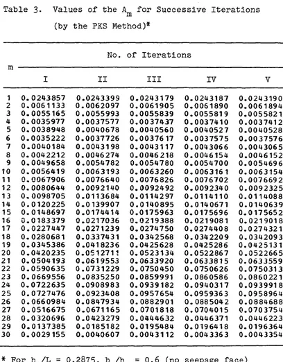
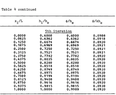
Table 3 gives values of the at successive iterations,
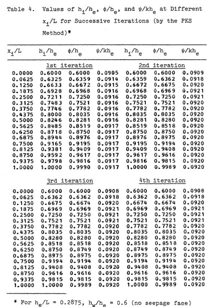
computed by the PKS method. Five iterations were used. Table
4 gives the hu/h^ and <J)(•x^/h^)/h^ for different values of
at successive iterations, computed by the PKS method. A
comparison of the results of last iterations in Tables 2 and
4 indicates a good agreement.
Case of seepage face It is interesting to note how
the length of the seepage face stabilizes in a few iterations.
Fig. 5 shows plots of h^/h^ versus number of iterations for
the simultaneous equations method and the PKS method. The
hg/h^, by the two methods, converges to the same final value.
The difference between the h /h after fourth and fifth s e
iterations (0.15168 and 0.15176) is considered negligible.
For better results, a greater number of the in the Fourier
series of equation [15] should be used. We have used 30
values of Bp.
A comparison of the heights of our free surface with
Murray's computations has been made in Fig. 6. His free
surface curve lies over ours except in close proximity of
x^/L = 0.
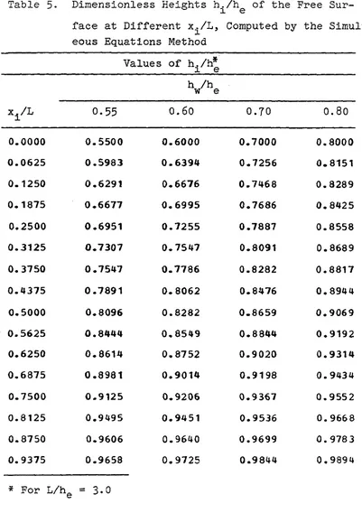
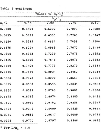
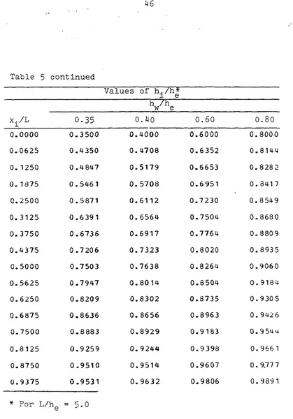
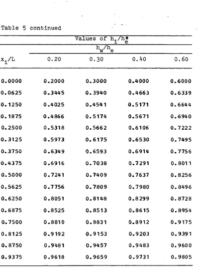
Table 5 has been prepared to give heights of the free
surface h^/h^ at different x^/L for the geometrical parameters
Table 3. Values of the A for Successive Iterations m
(by the PKS Method)*
No. of Iterations
m
I II Ill IV V
1 0. 0243857 0 .0243399 0. 0243179 0. 0243187 0. 0243190 2 0. 0061133 0 .0062097 0. 0061905 0. 0061890 0. 0061894 3 0. 0055165 0 .0055993 0. 0055839 0. 0055819 0. 0055821 4 0. 0035977 0 .0037577 0. 0037437 0. 0037410 0. 0037412 5 0. 0038948 0 .0040678 0. 0040560 0. 0040527 0. 0040528 6 0. 0035222 0 .0037726 0. 0037617 0. 0037575 0. 0037576 7 0. 0040184 0 .0043198 0. 0043117 0. 0043066 0. 0043065 8 0. 0042212 0 .0046274 0. 0046218 0. 0046154 0. 0046152 9 0. 0049658 0 .0054782 0. 0054780 0. 0054700 0. 0054696 10 0. 0056419 0 .0063193 0. 0063260 0. 0063161 0. 0063154 11 0. 0067906 0 .0076640 0. 0076826 0. 0076702 0. 0076692 12 0. 0080644 0 .0092140 0. 0092492 0. 0092340
0 .
0092325 13 0. 0098705 0 .0113684 0. 0114297 0. 01141100 .
0114088 14 0. 0120225 0 .0139907 0. 0140895 0. 0140671 0. 0140639 15 0. 0148697 0 .0174414 0. 0175963 0. 0175696 0. 0175652 16 0 . 0183379 0 .0217036 0. 0219388 0. 0219081 0. 0219018 17 0. 0227447 0 .0271239 0. 0274750 0. 0274408 0. 0274321 18 0. 0280681 0 .0337431 0. 0342568 0. 0342209 0. 0342093 19 0. 0345386 0 .0418236 0. 0425628 0. 0425286 0. 0425131 20 0. 0420235 0 .0512711 0. 0523134 0. 0522867 0. 0522665 21 0. 0504193 0 .0619553 0. 0633920 0. 0633815 0. 0633559 22 0. 0590635 0 .0731229 0. 0750450 0. 0750626 0. 0750313 23 0. 0669556 0 -0835250 0. 0859991 0. 0860586 0. 0860221 24 0. 0722635 0 .0908983 0. 0939182 0. 0940317 0. 0939918 25 0. 0727476 0 .0923408 0. 0957654 0. 0959363 0. 0958964 26 0. 0660984 0 .0847934 0. 0882901 0. 0885042 0. 0884688 27 0. 0516675 0 .0671165 0. 0701818 0. 0704015 0. 0703754 28 0. 0320696 0 .0423279 0. 0444632 0. 0446371 0. 0446223 29 0. 0137385 0 .0185182 0. 0195484 0. 0196418 0. 0196364 30 0. 0029155 0 .0040607 0. 0043112 0. 0043363 0. 0043354 [image:45.588.113.521.81.603.2]38
Table 4. Values of h^/h^, ^/h^, and Tp/kh^ at Different
x^/L for Successive Iterations (by the PKS
Method)*
x^/L h^/h^ 4/hg ^/kh^
1st iteration 2nd iteration
0. 0000 0. 6000 0. 6000 0. 0905 0. 6000 0. 6000 0. 0909 0. 0625 0. 6325 0. 6359 0. 0914 0. 6359 0. 6362 0. 0918 0. 1250 0. 6633 0. 6672 0. 0915 0. 6672 0. 6675 0. 092 0 0. 1875 0. 6928 0. 6968 0. 0916 0. 6968 G. 696 9 0. 0921 0. 2500 0. 721 1 0. 7250 0. 0916 0. 7250 0. 7250 0. 0921 0. 3125 0. 7483 0. 7521 0. 0916 0. 7521 0. 7521 0. 0920 0. 3750 0. 7746 0. 7782 0. 0916 0. 7782 0. 7782 0. 0920 0. 4375 0. 8000 0. 8035 0. 0916 0. 8035 0. 8035 0. 0920 0. 5000 0. 824 6 0. 8281 0. 0916 0. 8281 0. 8280 0. 0920 0. 5625 0. 8485 0. 8519 0. 0917 0. 8519 0. 8518 0. 0920 0. 6250 0. 8718 0. 8750 0. 0917 0. 8750 0. 8750 0. 0920 0. 6875 0. 8944 0. 8976 0. 0917 0. 8976 0. 8975 0. 0920 0. 7500 0. 9165 0. 9195 0. 0917 0. 9195 0. 9194 0. 0920
0.
8125 0. 9381 0. 9409 0. 0917 0. 9409 0. 9408 0. 0920 0. 8750 0. 9592 0. 9617 0. 0917 0. 9617 0. 9616 0. 0920 0. 93750.
9798 0. 9816 0. 0917 0. 9816 0. 9815 0. 0920 1. 0000 1. 0000 0. 9990 0. 0917 1. 0000 0. 9989 0. 09203rd iteration 4th iteration
0. 0000 0. 6000 0. 6000 0. 0908 0. 6000 0. 6000 0. 0908 0. 0625 0. 6362 0. 6362 0. 0918 0. 6362 0. 6362 0. 0918 0. 1250 0. 6675 0. 6674 0. 0920 0. 6674 0. 6674 0. 0920 0. 1875 0. 6969 0. 6969 0. 0921 0. 6969 0. 6969 0. 0921 0. 2500 0. 7250 0. 7250 0. 0921 0. 7250 0. 7250 0. 0921 0. 3125 0. 7521 0. 7521 0. 0921 0. ,7521 0. 7521 0. 0921 0. 3750 0. 7782 0. 7782 0. 0920 0. ,7782 0. 7782 0. 0920 0. 4375 0. 8035 0. 8035 0. 0920 0. .8035 0. 8035 0. 0920 0, 5000 0.8280 0. ,8280 0. 0920 0. 8280 0. 8280 0. 0920 0. 5625 0. ,8518 0. 8518 0. 0920 0.8518 0. 8518 0. 0920 0.6250 0. .8750 0, ,8749 0. 0920 0. ,8749 0. 874 9 0. 0920 0. ,6875 0. , 8975 0. ,8975 0. ,0920 0. .8975 0, 8975 0. ,0920 0. ,7500 0. .9194 0. ,9194 0. 0920 0. .9194 0. 9194 0. 0920 0. ,8125 0, ,9408 0. 9408 0. 0920 0. .9408 0. 9408 0. .0920 0, ,8750 0. .9616 0. .9616 0. ,0920 0, .9616 0. 9616 0, ,0920 0. 9375 0.9815 0.9815 0. ,0920 0. .9815 0. ,9815 0.0920 1. .0000 1, .0000 0. . 9989 0. ,0920 1, .0000 0, ,9989 0. ,0920
[image:46.599.122.541.71.684.2]Table 4 continued
x^/L hu/hg */hg Tlf/khg
0.0000 0.0625 0.1250 0.1875 0.2500 0.3125 0.3750 0.4375 0.5000 0.5625 0.6250 0.6875 0.7500 0.8125 0.8750 0.9375 1.0000 5th 0.6000 0.6362 0.6674 0.6969 0.7250 0.7521 0.7782 0.8035 0.8280 0.8518 0.8749 0.8975 0.9194 0.9408 0.9616 0.9815
1 . 0 0 0 0
Figure 5. Curves of h^/h^, computed by the PKS method and
the simultaneous equation method, drawn against
number of iterations for h^/L = 0.2875 and
.16
PKS method
0.15168
.15
0.1 5176
0.15282
.14
simultaneus equation method
.12
starting value
.10
Figure 6. A comparison of heights of the free surfaces as
computed by Murray^ the PKS Method and the
h J L
=0.2875
Vil, =0
— PKS method
X simultaneous equations
method
o Murray's results
="±17777777777777777777777777777777777777777^77
44
Table 5- Dimensionless Heights hu/h^ of the Free Sur
face at Different x^/L, Computed by the Simultan eous Equations Method
Values of h^/h*
x^/L 0.55 0 . 6 0 0.70 0 . 8 0
0.0000 0.5500 0.6000 0.7000 0.8000
0.0625 0.5983 0.6394 0.7256 0.8151
0.1250 0.6291 0.6676 0.7468 0.8289
0.1875 0.6677 0.6995 0.7686 0.8425
0.2500 0.6951 0.7255 0.7887 0.8558
0.3125 0.7307 0.7547 0.8091 0.8689
0.3750 0.7547 0.7786 0.8282 0.8817
0.4375 0.7891 0.8062 0.8476 0.8944
0.5000 0.8096 0.8282 0.8659 0.9069
0.5625 0.8444 0.8549 0.8844 0.9192
0.6250 0.8614 0.8752 0.9020 0.9314
0.6875 0.8981 0.9014 0.9198 0.9434
0.7500 0.9125 0.9206 0.9367 0.9552
0.8125 0.9495 0.9451 0.9536 0.9668
0.8750 0.9606 0.9640 0.9699 0.9783
0.9375 0.9658 0.9725 0.9844 0.9894
Table 5 continued
Values of h./h* 1 e
V'e
x^/L 0.45 0.60 0.70 0.80
0.0000 0.4500 0.6000 0.7000 0. 8000
0.0625 0.5133 0.6365 0.7243 0.8147
0.1250 0.5535 0.6661 0.7458 0. 8284
0.1875 0.6024 0. 6965 0.7672 0.8419
0.2500 0.6373 0.7239 0.7875 0.8552
0.3125 0.6805 0.7516 0.8076 0.8683
0.3750 0.7108 0.7773 0.8270 0.8811
0.4375 0.7510 0.8031 0.8462 0.8938
0.5000 0.7773 0.8272 0.8648 0.9063
0.5625 0.8160 0.8515 0.8831 0.9187
0.6250 0.8391 0.8743 0.9009 0.9308
0.6875 0.8775 0.8974 0.9185 0.9428
0.7500 0.8989 0.9192 0.9356 0.9547
0.8125 0.9343 0, 9409 0.9525 0.9664
0.8750 0.9553 0.9617 0.9689 0.9779
0.9375 0 .9770 0.9797 0.9848 0.989 2
[image:53.603.131.520.125.629.2]46
Table 5 continued
Values of h^/h*
x ^ / L 0.35 0.40 0.60 0.80
0 . 0 0 0 0
0.0625 0.1250 0.1875 0.2500 0.3125 0.3750 0.4375 0.5000 0.5625 0.6250 0.6875 0.7500 0.8125 0.8750 0.9375 0.3500 0.4350 0.4847 0.5461 0.5871 0.6391 0.5736
0 .7206
0.7503 0.7947 0.8209 0.8636 0.8883 0.9259 0-9510 0.9531 0.4000 0.4708 0.5179 0.5708 0.6112 0.6564 0.6917 0.7323 0.7638 0.8014 0.8302 0.8656 0.8929 0.9244 0.9514 0.9632 0.6000 0.6352 0.6653 0.6951 0.7230 0.7504 0.7764 0.8020 0.8264 0.8504 0.8735 0.8963 0.9183 0.9398 0.9607 0.9806 0.8000 0.8144
0 . 8 2 8 2
0.8417
0.8549
0.8680
Q. 880 9
0.8935
0.9060
0.9184
0.9305
0.9426
0. 9 54 4
0.966 1
0. 9.77 7
0.9891
..Table 5 continued
Values of h./h* 1 e
x^/L 0.35 o o 0.60 0.80
0.0000 0.3500 0.4000 0.6000 0.8000
0.0625 0.4309 0.4679 0.6344 0.8142
0.1250 0.4846 0.5175 0.6648 0.8279
0.1875 0.5425 0.5684 0.6945 0.8414
0.2500 0.5874 0.6109 0.7225 0.8547
0.3125 0.6355 0.6541 0.7498 0.8677
0.3750 0.6744 0.6916 0.7759 0.8806
0.4375 0.7168 0.7301 0,8014 0.8933
0.5000 0.7515 0.7639 0.8259 0.9058
0.5625 0.7901 0.7990 0,8499 0.9182
0.6250 0.8219 0.8302 0.8731 0.9303
0.6875 0.8574 0.8626 0.8 957 0.9423
0.7500 0.8875 0.8919 0.9178 0.9542
0.8125 0.9190 0.9213 0.9393 0.9659
0.8750 0.9481 0.9493 0.9603 0.9775
0.9375 0.9654 0.9709 0.9806 0.9889
48
Table 5 continued
Values of /h* e
x^/L 0.20 0 . 3 0 0.40 0.60
0.0000 0.2000 0.3000 0.4000 0.6000
0.0625 0.3445 0.3940 0.4663 0.6339
0.1250 0.4025 0.4541 0.5171 0.6644
0.1875 0.4866 0.5174 0.5671 0.6940
0.2500 0.5318 0.5662 0.6106 0.7222
0.3125 0.5973 0.6175 0.6530 0.7495
0.3750 0.6349 0.6593 0.6914 0.7756
0.4375 0.6916 0.7038 0.7291 0.8011
0.5000 0.7241 0.7409 0.7637 0.8256
0.5625 0.7756 0.7809 0.7980 0.8496
0.6250 0.8051 0.8148 0.8299 0.8728
0.6875 0.8525 0.8513 0.8615 0.8954
0.7500 0.8810 0.8831 0.8912 0.9175
0.8125 0.9192 0.9153 0.9203 0.9391
0.8750 0.9481 0.9457 0.9483 0.9600
0.9375 0.9618 0.9659 0.9731 0.9805
values of L/h^ and h^/h^, not included in this table, inter
polation of the tabulated values is recommended. The extra
polation, however, is unsafe. An example illustrating the
interpolation of values from Table 5 follows.
Example It is desired to determine the height of the
free surface h^ at x^ = 1.5 ft when h^ = 2.875 ft, h^ =
1.725 ft and L = 10.0 ft. L/h^ = 10/2.875 = 3-4783, x^/L =
0.15, and h /h^ = 1.725/2.875 = 0.6.
From Table 5, we extract, for by/h^ = 0.6, the following
values.
x./L L/hg hu/hg
0.125 3.0 0.66757
0 . 1 2 5 4 . 0 0 . 6 6 6 0 9
0 . 1 2 5 5 . 0 0 . 6 6 5 2 5
0 . 1 8 7 5 3 . 0 0 . 6 9 9 5 2
0 . 1 8 7 5 4. 0 0.69645
0 . 1 8 7 5 5 . 0 0 . 6 9 5 1 4
0 . 2 5 0 3 . 0 0 . 7 2 5 4 6
0.250 4.0 0.72393
0.250 5.0 0.72304
Now we draw curves of h^/h^ versus L/h^ for x^/L = 0.125,
0.1875, and 0.25, and read the values of h^/h^ at L/h^ =
3.4783 from the resulting curves. The value so read are
Xj^/L h^/h^
0 . 1 2 5 0 . 6 6 6 8
0 . 1 8 7 5 0 . 6 9 7 7
0 . 2 5 0 . 7 2 4 6
Now a curve of h^/h^ versus x^/L is drawn from the above
50
curve. Finally = 0.6795 (2.875) = 1.954 ft.
Flownets
General expressions relating a normalized $*(x,y) with
and ^ normalized *'(x,y) with and may
be written as
(j)(x,y) - * .
4 ' ( x , y ) = *
[ 3 0 ]
max ^min
and
max ^min
For our problem, W = *mln = 0'
'''max ~ ^ where q is given by equation [3]. Equations [30] and
[31]J in view of the above-mentioned values, reduce to
*(x,y) - h
4'(x,y) = h - h— [32]
e w
and
^^(x,y) = [33]
Now, with Bp and computed from equation [9] and any of
the two iterative technique, respectively, $'(x,y) and ^^(x,y)
/
are computed from equations [6], [7], [32] and [33]. Con
sequently a flownet may be sketched or a computer simplotter
flownets.
Fig. 7 and 8 show flownets for the geometrical parameters;
h /L = 0.2875, h^/h^ =0.6; and h^/L = 0.2875, h^/h^ = 0,
respectively. Fig. 7 also shows some interesting features of
the fictitious flow region. The top horizontal boundary is
both a source and a sink. In other words, it is supplying
water to the fictitious flow region as well as receiving water
from it.
Extension to axisymmetric flow
Fig. 9 is a diagrammatic representation of a well of
diameter 2r^ drilled in an unconfined aquifer which is under
lain by a horizontal impermeable base. The aquifer has a
cylindrical outer boundary of diameter 2rg, concentric with
the well, such that the potential head at this boundary
remains constant. The aquifer is not recharged from the
ground surface. The water level in the well, which penetrates
the entire thickness of the aquifer down to the impermeable
barrier, remains constant. In other words, the water flowing
into the well by gravity is removed instantaneously by pump
ing or other means.
A system of axisymmetric cylindrical coordinates (r,z)
is established, as shown in Fig. 9 and the impermeable barrier
is chosen as the datum for the measurement of hydraulic poten
tial. Laplace's equation, for a steady-state flow, in axisym
Figure 7. A flownet of unconflned flow between two parallel ditches for
1^ = 0.4
^=0.2
U1
Figure 8. A flownet of unconflned flow between two parallel ditches for
h / h = 0 a n d h / L = 0 . 2 8 7 5 ( w h e n s e e p a g e f a c e I s s i g n i f i c a n t )
Figure 9. Diagrammatic representation of an unconfined flow
seepage
|
face V
welk
free surface
D
2
h^2
A
^ L ' L
n f u n n u / i f n u i r f u r n t t i n n n n n i n n i n n n r n n n n
58
A
+ + ° [34]3r 3z
A potential function (j)(r,z) and a stream function )|)(r,z)
for our flow region can be developed by solving equation [34]
to satisfy the following boundary condtions (see Fig. 9)
Along OA Tj; = 0 or 3(t)/3r =0 BC 1
Along AB (j) = hg BC 2
Along BC ({) = h(r) BC 3
= Q/2ir BC 4
Along CD (j> = z BC 5
Along OD <f) = h^ BC 6
where Q is the well discharge. Again, Dupuit-Forchheimer
theory happens to give an exact formula for the well dis
charge. The formula is
« = C351
Now following the development of <)> and ^ for the
two-dimensional flow, and using the general solution of equation
[34] and Cauchy-Riemann relations, given by Kirkham and Powers
(1972, p. 128) we can write $ and for this problem, by in
^
^ - : BpRoCBpDcos BpZcosh(v z)
+ : V cosh(v"h^) =o(V) [36]
= rl in(vC '
% '
Vl'V>
sinh(v z)
#; ^ \ cosh(v°h^) =l(V> [37]
where Bp and are as defined already by equations [5] and
[9], respectively5 and are arbitrary constants, and
R
q,C
q,R
^5 and are defined by= Jo<Vw' Jo(V) [39]
RjCB r) =
%(Bpr) - IiCgpf) K„(epr^)
and
[10]
Cl(Vnf) [11]
In equations [36] to [41], Iq, Kq, Jq, Yq, K^,
60
To satisfy boundary condition 2, must be positive
real roots of the equation
The first 40 roots of equation [39] are tabulated in Khan
et al. (1971) (their u^ equal our ~
All the boundary conditions of the real flow region ex
cept that at the free surface are satisfied. To apply BC 3,
we put (j) = hj^, 2 = hj^, and r = r^ in equation [36] to get
^i _ ^s . - E B R ($ r.)cos 3 h.
cosh(v h. )
+ % cosh(v^hJ =0<Vl) [43]
In order to apply BC 4, we put z = h^, r = r^, and jp =
Q/2Tr in equation [37]. The resulting expression, after
putting right side of equation [35] for Q and rearranging,
yields
2 hX intre/r*) " ^
r. sinh(v h.)
= ^ GOshCv^hg) ^l^Vi)