SCALABLE AND ROBUST CLUSTERING AND VISUALIZATION FOR LARGE SCALE BIOINFORMATICS DATA

(1)

SCALABLE AND ROBUST CLUSTERING AND

VISUALIZATION FOR LARGE-SCALE

BIOINFORMATICS DATA

Yang Ruan

Submitted to the faculty of the University Graduate School in partial fulfillment of the requirements

for the degree Doctor of Philosophy

in the Department of Computer Science Indiana University

(2)

Accepted by the Graduate Faculty, Indiana University, in partial fulfillment of the requirements of the degress of Doctor of Philosophy.

Doctoral

Committee Geoffrey C. Fox

(Principal Advisor)

David Leake

Judy Qiu

August 18, 2014

(3)

(4)

There are no secrets to success. It is the result of preparation, hard work, and learning from failure.

(5)

Acknowledgements

First of all, I am sincerely grateful to my adviser Professor Geoffrey C. Fox, for his farsighted guidance, insightful advice, and unlimited support during the past years. His guidance pointed out to me the correct way of doing research as a scientist in this dissertation as well as in my other research projects. On the basis of his patience and valuable advice, I significantly increased my knowledge as I work toward the PhD degree.

It is my great pleasure to thank the members of my research committee: Professor Judy Qiu, Professor Haixu Tang and Professor David Leake. I cannot overstate their invaluable comments that helped me understand and solve the research issues. These suggestions given by them greatly expanded my vision in the area of research.

It is been a pleasure working for various projects at SALSA HPC group in Community Grid Lab. I enjoyed the weekly discussions with Professor Judy Qiu and my colleagues: Dr. Jaliya Ekanayake, Dr. Thilina Gunarathne, Xiaoming Gao, Saliya Ekanayake, Bingjing Zhang, Tak-Lon Wu, Hui Li, Fei Teng, Yuduo Zhou, Jerome Mitchell, Adam Hughes, and Scott Beason. The collaboration with my friendly and brilliant colleagues greatly expanded my horizon. Especially, I want to thank Dr. Zhenhua Guo, for his invaluable and electrifying discussions with me on various research topics.

I would like to thank the administrative support from School of Informatics and Computing, FutureGrid, and University Information Technology Services. Because of their help, I am able to finish many research projects in time.

Finally, I want to thank my father Shanqing Ruan and my mother Xiaobin Guo, for their generous support during the past few years. I would not be able to finish the Doctor degree without their endless love and support.

Again, I am deeply grateful for all your support!

(6)

Abstract

(7)

L

IST OF

T

ABLES

TABLE 1SUMMARY OF THE ALGORITHMS PROPOSED IN THIS DISSERTATION ... 9

TABLE 2THE DATASET USED IN THE EXPERIMENTS ACROSS THE DISSERTATION ... 38

TABLE 3ALL 4 ALGORITHMS TESTED IN FOLLOWING EXPERIMENTS ... 38

TABLE 4THE LIST OF DATA BEING USED IN FOLLOWING EXPERIMENTS ... 83

(11)

L

IST OF

F

IGURES

FIGURE 1.1: ILLUSTRATIONS OF INTERPOLATE OUT-OF-SAMPLE POINTS INTO THE IN-SAMPLE

TARGET DIMENSION SPACE AS 2D. ... 5

FIGURE 2.1:ILLUSTRATION OF CALCULATING PID BETWEEN TWO ALIGNED SEQUENCES ... 12

FIGURE 2.2:VISUALIZATION OF 16S RRNA DATA WITH NW PAIRWISE SEQUENCE ALIGNMENT RESULT... 13

FIGURE 2.3: VISUALIZATION OF 16S RRNA WITH SWG PAIRWISE SEQUENCE ALIGNMENT RESULT... 13

FIGURE 2.4:PARALLELIZATION OF THE ASA PROBLEM.THE TOTAL NUMBER OF SEQUENCE IS N, AND THE DARKER BLOCK IS THE BLOCK NEEDS TO BE PROCESSED, AND WHITE BLOCKS ARE THEIR SYMMETRIC BLOCKS. ... 15

FIGURE 2.5:2D TREE DIAGRAM EXAMPLE FOR 5 SEQUENCES, LEFT ONE IS THE RECTANGULAR CLADOGRAM, AND RIGHT ONE IS THE RECTANGULAR PHYLOGRAM ... 20

FIGURE 2.6:THE FLOWCHART OF DACIDR OF PROCESSING OVER MILLIONS OF SEQUENCES UNTIL THE PHYLOGENETIC TREE IS VISUALIZED BASED ON PREVIOUS EXPERIENCE. ... 22

FIGURE 3.1: THE FLOWCHART OF PARALLEL WDA-SMACOF USING AN ITERATIVE

MAPREDUCE FRAMEWORK ... 31

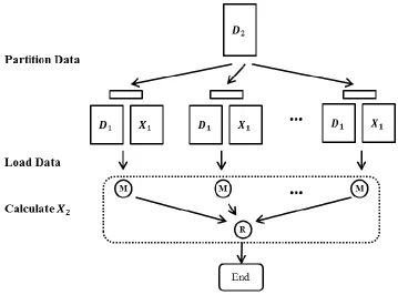
FIGURE 3.2:GRAPH REPRESENTATION OF DIVIDING X INTO X1 AND X2 ... 33

(12)

FIGURE 3.4:GRAPH REPRESENTATION OF DIVIDING B(Z) INTO 4 PARTS ... 33

FIGURE 3.5: THE FLOWCHART OF PARALLEL FIXED-WDA-SMACOF USING AN ITERATIVE

MAPREDUCE FRAMEWORK ... 36

FIGURE 3.6:THE NORMALIZED STRESS VALUE COMPARISON BETWEEN 4MDS ALGORITHMS USING 2000ARTIFICIAL RNA SEQUENCES.ALL 4 ALGORITHMS IN THIS EXPERIMENT ARE SEQUENTIAL. ... 42

FIGURE 3.7: THE CLUSTERING AND VISUALIZATION RESULT OF ENTIRE ARTIFICIAL RNA

DATASET WITH 13 CLUSTERS LABELED.EACH POINTS BELONGS TO THE SAME COLOR IS A CLUSTER FOUND BY USING DA-PWC PROGRAM. ... 42

FIGURE 3.8:THE NORMALIZED STRESS VALUE COMPARISON BETWEEN 4MDS ALGORITHMS USING 4872COG CONSENSUS SEQUENCES.ALL 4 ALGORITHMS IN THIS EXPERIMENT ARE SEQUENTIAL. ... 43

FIGURE 3.9:THE CLUSTERING AND VISUALIZATION RESULT OF ENTIRE COG DATASET WITH A FEW CLUSTERS LABELED. THESE CLUSTERS WERE MANUALLY DEFINED BY USING THE INFORMATION FROM NIH. ... 43

FIGURE 3.10:THE NORMALIZED STRESS VALUE COMPARISON BETWEEN 4MDS ALGORITHMS USING 10K HMP 16S RRNA SEQUENCES.ALL 4 ALGORITHMS IN THIS EXPERIMENT ARE PARALLELIZED USING TWISTER ON 80 CORES. ... 44

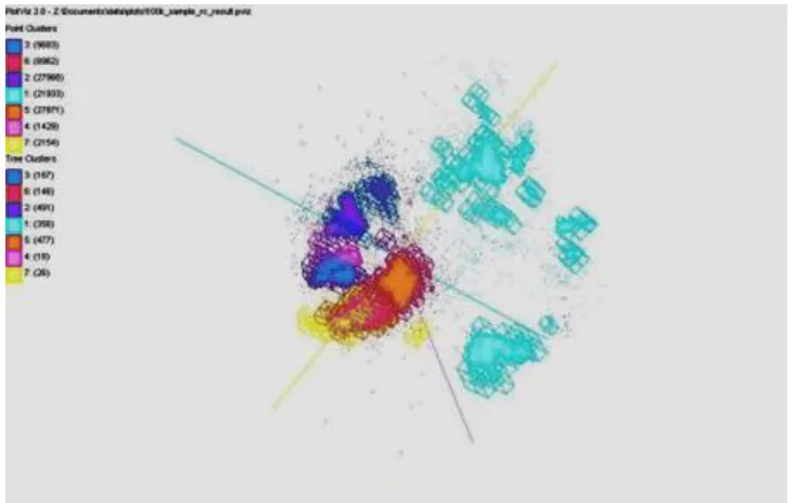
FIGURE 3.11: THE CLUSTERING AND VISUALIZATION RESULT OF ENTIRE HMP16S RRNA

(13)

FIGURE 3.12:THE NORMALIZED STRESS VALUE COMPARISON BETWEEN 4MDS ALGORITHMS USING 100K AM FUNGAL SEQUENCES.ALL 4 ALGORITHMS IN THIS EXPERIMENT ARE PARALLELIZED USING TWISTER ON 600 CORES. ... 45

FIGURE 3.13:THE CLUSTERING AND VISUALIZATION RESULT OF ENTIRE AM FUNGAL DATASET WITH 10 MEGA REGIONS LABELED. EACH POINTS BELONGS TO THE SAME COLOR IS A MEGA REGION FOUND BY USING DA-PWC PROGRAM. ... 45

FIGURE 3.14: THE TIME COST COMPARISON BETWEEN 4 MDS ALGORITHMS USING 2000 ARTIFICIAL RNA SEQUENCES. ALL 4 ALGORITHMS IN THIS EXPERIMENT ARE SEQUENTIAL. ... 48

FIGURE 3.15:THE TIME COST COMPARISON BETWEEN 4MDS ALGORITHMS USING 10K HMP 16S

RRNA SEQUENCES.ALL 4 ALGORITHMS IN THIS EXPERIMENT ARE PARALLELIZED USING

TWISTER ON 80 CORES. ... 49

FIGURE 3.16:THE TIME COST COMPARISON BETWEEN 4MDS ALGORITHMS USING 4872COG

CONSENSUS SEQUENCES.ALL 4 ALGORITHMS IN THIS EXPERIMENT ARE SEQUENTIAL. ... 49

FIGURE 3.17:THE NORMALIZED STRESS WITH INCREASING NUMBER OF ITERATIONS BETWEEN A WEIGHTED MDS ALGORITHM WDA-SMACOF AND A NON-WEIGHTED MDS

ALGORITHM, NDA-SMACOF. THE NDA-SMACOF (T) IS THE ACTUAL NORMALIZED

STRESS VALUE THAT CALCULATED USING THE WEIGHT MATRIX, WHERE NDA-SMACOF IS THE STRESS VALUE WITH WEIGHTS ALL EQUAL 1. ... 50

FIGURE 3.18:THE TIME COST OF WDA-SMACOF AND NDA-SMACOF PROCESSING 10K HMP

(14)

FIGURE 3.19:THE TIME COST OF CG VERSUS MATRIX INVERSE OVER 1K TO 8K HMP 16S RRNA

DATA. THE MATRIX INVERSION USES CHOLESKY DECOMPOSITION AND CG USES 20

ITERATIONS.BOTH ALGORITHMS WERE SEQUENTIAL. ... 53

FIGURE 3.20: THE NUMBER OF CG ITERATION NEEDED FOR 100K AM FUNGAL DATA PROCESSED WITH PARALLEL WDA-SMACOF.THE PERCENTAGE OF MISSING DISTANCES INCREASES FROM 0 TO 0.5 AND ALL MISSING DISTANCES ARE RANDOMLY CHOSEN. ... 54

FIGURE 3.21: THE NUMBER OF CG ITERATION NEEDED FOR AM FUNGAL DATA PROCESSED WITH PARALLEL WDA-SMACOF. THE DATA SIZE VARIES FROM 20K TO 100K. THE NUMBER OF ITERATIONS TOOK OVER THE AVERAGE OF NUMBER OF CG ITERATIONS FROM THE SCENARIOS THAT PERCENTAGE OF MISSING DISTANCES INCREASES FROM 0 TO

0.5. ... 54

FIGURE 3.22:THE NUMBER OF CG ITERATION NEEDED FOR 2K ARTIFICIAL RNA DATA,4872 CGOPROTEIN DATA AND 10K HMP16S RRNA DATA PROCESSED WITH PARALLEL WDA-SMACOF WITH SAMMON'S MAPPING. ... 55

FIGURE 3.23: THE NUMBER OF CG ITERATION NEEDED FOR AM FUNGAL DATA PROCESSED WITH PARALLEL WDA-SMACOF WITH SAMMON'S MAPPING.THE DATA SIZE INCREASES FROM 20K TO 100K. ... 55

FIGURE 3.24:TIME COST OF WDA-SMACOF WITH EQUAL WEIGHTS COMPARED WITH WDA-SMACOF WITH SAMMON'S MAPPING USING AM FUNGAL DATA. THE DATA SIZE INCREASES FROM 20K TO 100K.EACH RUN TAKES 100SMACOF ITERATIONS. ... 56

(15)

FIGURE 3.26:THE TIME COST PROPORTION EACH STEPS OF PARALLEL WDA-SMACOF.THE DATA SIZE AND NUMBER OF PROCESSORS VARY... 59

FIGURE 3.27:THE TIME COST PROPORTION IN ONE SMACOF ITERATION OF PARALLEL WDA-SMACOF WITH 100K AMFUNGAL DATA BY INCREASING NUMBER OF PROCESSORS. ... 60

FIGURE 3.28:THE AVERAGE TIME COST OF THE SINGLE MAPREDUCE JOB FOR THREE CORE STEPS IN PARALLEL WDA-SMACOF WITH INCREASING AM FUNGAL DATA SIZE. ... 60

FIGURE 3.29:THE TIME COST OF PARALLEL WDA-SMACOF PROCESSING 100K AMFUNGAL DATA WITH NUMBER OF PROCESSORS INCREASED FROM 512 TO 4096. ... 61

FIGURE 3.30: THE PARALLEL EFFICIENCY OF PARALLEL WDA-SMACOF PROCESSING 100K

AMFUNGAL DATA WITH NUMBER OF PROCESSORS INCREASED FROM 512 TO 4096. ... 61

FIGURE 3.31:THE NORMALIZED STRESS VALUE COMPARISON OF WDA-SMACOF AND MI-MDS.THE IN-SAMPLE DATA COORDINATES ARE FIXED, AND REST OUT-OF-SAMPLE DATA COORDINATES CAN BE VARIED. ... 63

FIGURE 3.32: THE TIME COST COMPARISON OF WDA-SMACOF AND MI-MDS. THE IN

-SAMPLE DATA COORDINATES ARE FIXED, AND REST OUT-OF-SAMPLE DATA COORDINATES CAN BE VARIED. ... 63

FIGURE 4.1:THE FLOWCHART OF PARALLEL W-MI-MDS USING AN MAPREDUCE FRAMEWORK

... 71

(16)

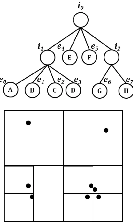
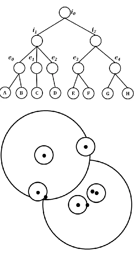
FIGURE 4.3:AN ILLUSTRATION OF CN-TREE WITH 8 SEQUENCES.THE UPPER CHART IS THE TREE RELATIONSHIPS, AND CHART BELOW IS THE ACTUAL REPRESENTATION OF SSP-TREE IN HYPERSPACE AND PROJECTED TO 2D. ... 77

FIGURE 4.4:THE TERMINAL NODES GENERATED FOR 100K AMFUNGAL DATA IN 3D FROM SSP-TREE USING HE-MI ALGORITHM. THE DIFFERENT COLORS REPRESENTS DIFFERENT MEGA REGIONS. ... 79

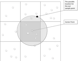
FIGURE 4.5: THE 2D EXAMPLE FOR INTERPOLATING AN OUT-OF-SAMPLE POINT INTO IN

-SAMPLE SPACE WITH SSP-TREE.THE WHITE POINTS ARE IN-SAMPLE POINTS AND THE BLACK POINT IS THE OUT-OF-SAMPLE POINTS.THE BLACK CIRCLE MEANS THE POSSIBLE POSITION OF THE OUT-OF-SAMPLE POINT AND THE DASHED CIRCLE IS THE POSSIBLE AREA FOR THE NEAREST NEIGHBORS OF THAT OUT-OF-SAMPLE POINT. ... 80

(17)

RNA SEQUENCES AS OUT-OF-SAMPLE DATA. ALL 4 ALGORITHMS IN THIS EXPERIMENT ARE SEQUENTIAL. ... 86

FIGURE 4.9:THE NORMALIZED STRESS VALUE COMPARISON BETWEEN 4MDS ALGORITHMS USING 10K HMP16SRRNA SEQUENCES AS IN-SAMPLE DATA, AND 40K HMP16SRRNA

SEQUENCES AS OUT-OF-SAMPLE DATA. ALL 4 ALGORITHMS IN THIS EXPERIMENT ARE PARALLEL ALGORITHMS USING 80 CORES. ... 86

FIGURE 4.10:THE NORMALIZED STRESS VALUE COMPARISON BETWEEN 4MDS ALGORITHMS USING 4872 CONSENSUS SEQUENCES AS IN-SAMPLE DATA, AND 95672COG SEQUENCES AS OUT-OF-SAMPLE DATA. ALL 4 ALGORITHMS IN THIS EXPERIMENT ARE PARALLEL ALGORITHMS USING 40 CORES. ... 87

FIGURE 4.11: THE TIME COST COMPARISON BETWEEN 4 MDS ALGORITHMS USING 2000 ARTIFICIAL RNA SEQUENCES AS IN-SAMPLE DATA, AND 2640 ARTIFICIAL RNA

SEQUENCES AS OUT-OF-SAMPLE DATA. ALL 4 ALGORITHMS IN THIS EXPERIMENT ARE SEQUENTIAL. ... 90

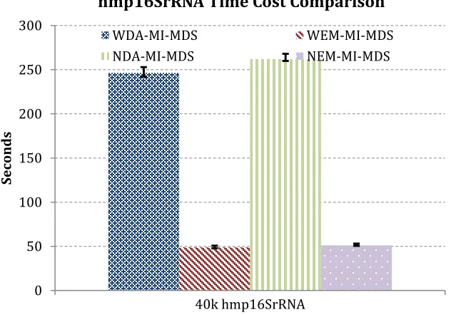
FIGURE 4.12: THE TIME COST COMPARISON BETWEEN 4 MDS ALGORITHMS USING 10K HMP16SRRNA SEQUENCES AS IN-SAMPLE DATA, AND 40K HMP16SRRNA SEQUENCES AS OUT-OF-SAMPLE DATA. ALL 4 ALGORITHMS IN THIS EXPERIMENT ARE PARALLEL ALGORITHMS USING 80 CORES. ... 90

(18)

FIGURE 4.14:THE TIME COST OF W-MI-MDS AND MI-MDS PROCESSING 40K HMP 16S RRNA

DATA INTERPOLATING TO 10K HMP 16S RRNA USING 80 CORES BY FIXING THE ITERATION TO 50 AND INCREASES THE PERCENTAGE OF MISSING DISTANCES RANDOMLY. ... 91

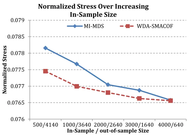
FIGURE 4.15:THE TIME COST COMPARISON OF 4MDS INTERPOLATION METHODS USING 100K HMP16SRRNA DATA, AND DIVIDED INTO IN-SAMPLE AND OUT-OF-SAMPLE DATASETS.THE IN-SAMPLE DATASET INCREASES WHILE OUT-OF-SAMPLE DECREASES. ... 93

FIGURE 4.16: THE NORMALIZED STRESS VALUE COMPARISON OF 4 MDS INTERPOLATION METHODS USING 100K HMP16SRRNA DATA, AND DIVIDED INTO IN-SAMPLE AND OUT-OF

-SAMPLE DATASETS. THE IN-SAMPLE DATASET INCREASES WHILE OUT-OF-SAMPLE DECREASES. ... 93

FIGURE 5.1:THE LEFT HAND SIDE OF THE GRAPH REPRESENTATION IS A CUBIC CLADOGRAM DISPLAYED WITH 8 SEQUENCES.THE RIGHT HAND SIDE OF THE GRAPH IS THE SAME 8

SEQUENCES VISUALIZED IN 2D AFTER DIMENSION REDUCTION. ... 99

FIGURE 5.2:THE EXAMPLE OF CHOOSING A RANDOM LINE TO PROJECT ALL THE SEQUENCES TO AND DRAW THE GIVEN CUBIC CLADOGRAM ACCORDINGLY. ... 100

FIGURE 5.3: AN EXAMPLE OF A GOOD CHOICE OF PROJECTION LINE AS THE DOTTED LINE WITHIN 8 SEQUENCES VISUALIZED IN 2D SPACE. ... 100

FIGURE 5.4:THE EXAMPLE OF CHOOSING A GOOD PROJECTION LINE DETERMINED BY PCA TO PROJECT ALL THE SEQUENCES TO AND DRAW THE GIVEN CUBIC CLADOGRAM

ACCORDINGLY. ... 101

(19)

FIGURE 5.6:THE VISUALIZATION RESULT OF 599NTS DATA USING MSA AND WDA-SMACOF ... 108

FIGURE 5.7:THE SCREEN SHOT FROM THE SIDE OF THE CUBOID CLADOGRAM BY CHOOSING A PLANE USING PCA ON 599NTS DATA USING MSA AND WDA-SMACOF ... 109

FIGURE 5.8:THE SCREEN SHOT FROM THE BOTTOM OF THE CUBOID CLADOGRAM BY CHOOSING A PLANE USING PCA ON 599NTS DATA USING MSA AND WDA-SMACOF ... 109

FIGURE 5.9:THE SCREEN SHOT FROM THE TOP OF THE CUBOID CLADOGRAM BY CHOOSING A PLANE USING PCA ON 599NTS DATA USING MSA AND WDA-SMACOF ... 110

FIGURE 5.10:MAXIMUM LIKELIHOOD PHYLOGENETIC TREE FROM 599NTS THAT IS COLLAPSED INTO CLADES AT THE GENUS LEVEL AS DENOTED BY COLORED TRIANGLES AT THE END OF

THE BRANCHES. BRANCH LENGTHS DENOTE LEVELS OF SEQUENCE DIVERGENCE BETWEEN GENERA AND NODES ARE LABELED WITH BOOTSTRAP CONFIDENCE VALUES.

454 SEQUENCES FROM SPORES THAT ARE NOT PART OF ANOTHER CLADE ARE DENOTED WITH THE LABEL ‘454 SEQUENCE FROM SPORE’.DISTANCE CALCULATION COMPARISON

... 111

FIGURE 5.11:THE SCREENSHOTS OF SPHERICAL PHYLOGRAM FOR USING THE PHYLOGENETIC TREE SHOWN IN FIGURE 5.10SWG PAIRWISE SEQUENCE ALIGNMENT.THE COLORS OF THE BRANCHES IN THESE FIGURES ARE AS SAME AS THE COLORS OF THE BRANCHES

SHOWN IN FIGURE 5.10. ... 112

FIGURE 5.12:THE SCREENSHOTS OF SPHERICAL PHYLOGRAM FOR USING THE PHYLOGENETIC TREE SHOWN IN FIGURE 5.10 MULTIPLE SEQUENCE ALIGNMENT.THE COLORS OF THE BRANCHES IN THESE FIGURES ARE AS SAME AS THE COLORS OF THE BRANCHES SHOWN IN

(20)

FIGURE 5.13: THE COMPARISON USING MANTEL BETWEEN DISTANCES GENERATED BY MSA

AND TWO PWA METHODS AND RAXML ... 114

FIGURE 5.14: MANTEL COMPARISON OF WDA-SMACOF, LMA AND EM-SMACOF USING DISTANCE INPUT GENERATED FROM ONE MSA METHOD AND TWO PWA METHODS ON

599NTS DATASET ... 117

FIGURE 5.15: MANTEL COMPARISON OF WDA-SMACOF, LMA AND EM-SMACOF USING DISTANCE INPUT GENERATED FROM ONE MSA METHOD AND TWO PWA METHODS ON

999NTS DATASET ... 117

FIGURE 5.16:SUM OF TREE BRANCHES IN 3D OF WDA-SMACOF,LMA AND EM-SMACOF

USING DISTANCE INPUT GENERATED FROM ONE MSA METHOD AND TWO PWA METHODS ON 599NTS DATASET ... 118

FIGURE 5.17:SUM OF TREE BRANCHES IN 3D OF WDA-SMACOF,LMA AND EM-SMACOF

USING DISTANCE INPUT GENERATED FROM ONE MSA METHOD AND TWO PWA METHODS ON 999NTS DATASET ... 118

FIGURE 5.18:THE PLOT OF 599NTS DATA USING LMAMDS METHOD ON MSA DISTANCES.THE RED SPHERE POINTS ARE THE TWO HIGHLIGHTED POINTS THAT ARE NEAR EACH OTHER

FROM THE PHYLOGENETIC TREE.THE BLUE SQUARE POINTS ARE SIMILAR POINTS THAT SHOULD BELONG TO A SAME FAMILY. ... 119

FIGURE 5.19: THE PLOT OF 599NTS DATA USING WDA-SMACOF METHOD ON MSA

(21)

Chapter 1.

I

NTRODUCTION

1.1 Sequence Clustering and Visualization

Advances in modern bio-sequencing techniques have led to a proliferation of raw genomic data that need to be analyzed with various technologies such as pyrosequencing [1, 2]. These technology enables biologist generate mass gene sequence fragments within a short period of time. However, many existing methods lack efficiency on massive sequence collections analysis where the existing computational power on single machine can be overwhelmed. Consequently, new techniques and parallel computation must be brought to this area.

(22)

methods were developed over past few years [5-7] . The key step among these methods is clustering, which is to group input sequences into different OTUs. However, most of these clustering methods require a quadratic space and time over the input sequence size. For example, hierarchical clustering is one of the most popular choices that have been widely used in many sequence analysis tools. It is a classic method, which is based on pairwise distance between input sequence samples. However, the main drawback of it is the quadratic space requirement for input distance matrix and a time complexity of O(N2). To overcome this shortage, several heuristic and hierarchical methods are developed and sometimes they can only perform on low dimensional data or lack accuracy [8, 9].

In order to visualize the clustering result from taxonomy-independent analysis in an intuitive way, dimension reduction techniques are used commonly in this field. It has been proved to be useful in data clustering and visualization field [5, 10]. This technique enables the investigation of unknown structures from high dimensional space into visualization in 2D or 3D space. Multidimensional Scaling [11] (MDS) is one set of techniques among many existing dimension reduction methods, such as Principal Component Analysis [12] (PCA) , Generative Topographic Mapping [13] (GTM), and Self-Organizing Maps [14] (SOM). Different from them, which focus on using the feature vector information in original dimension to construct a configuration in low dimension space, MDS focuses on using the proximity data, which is represented as pairwise dissimilarity values generated from high dimensional space. As in bioinformatics data, one needs to deal with sequences generated from sequencing technology, where the feature vectors are very difficult to be retrieved because of various sequence lengths. It is not suitable to use technologies other than MDS for their dimension reduction.

(23)

This dissertation is mainly focused on optimizing MDS techniques and applies MDS technique into various situations in order to help biologist visualize the clustering result better. New algorithm has been proposed to improve the overall accuracy of MDS technique, and some optimization techniques has been proposed in order to lower the time cost as well. Finally, this dissertation also describes some detailed performance analyses and experiments related to the proposed methodologies.

1.2 Multidimensional Scaling

Multidimensional Scaling (MDS) is a set of statistic techniques used in dimension reduction. It is a general term for these techniques to apply on original high dimensional data and reduce their dimensions to target dimension space while preserving the correlations, which is usually Euclidean distance calculated from the original dimension space from the dataset, between each pair of data points as much as possible. This is a non-linear optimization problem in terms of reducing the difference between the mapping of original dimension space and target dimension space. In bioinformatics data visualization, each sequence in the original dataset is considered as a point in both original and target dimension space. The dissimilarity between each pair of sequences is considered as Euclidean distance used in MDS.

Given a data set of points in original space, a pairwise distance matrix can be given from these data points ( ) where is the dissimilarity between point and point in original dimension space which follows the rules: (1) Symmetric: . (2) Positivity: . (3)

Zero Diagnosal: . Given a target dimension , the mapping of points in target dimension can be given by an matrix , where each point is denoted as from original space is represented as th row in .

The object function represents the proximity data for MDS to construct lower dimension space is called STRESS or SSTRESS, which are given in equation (1) and (2):

( ) ∑ ( ( ) )  

(24)

where denotes the possible weight from each pair of points that ,

denotes the Euclidean distance between point and in target dimension.

It is easy to learn that the STRESS or SSTRESS [20] value actually represents the difference of between the distance calculated from the original dimension and the distance calculated from the mapping in the target dimension. The optimization process of MDS technique is used to minimize this difference. When the difference is minimized, the mapping in the target dimension will preserve most of the information among the data. As for the visualization from bioinformatics sequences, the sequence clustering sometimes will emerge naturally in the dimensionality reduction result (3D space), where one can easily observe the sequence clusters intuitively.

1.3 Online MDS

The traditional MDS problem are usually solved in O(N2) time and space. This is because of the requirement from the input of MDS that usually requires distances between all pairs of sequences. This makes MDS techniques hard to be applied on very large scale dataset. As the data size explodes during the past few years because of the next generation sequencing [12] (NGS) techniques, it is essential to find alternative method to address this problem. And the in-sample and out-of-sample solution has been brought up in data clustering and visualization to solve the large-scale data problem [21]. In this scenario, the whole dataset is divided into two parts: one part is called in-sample dataset, and the other part is called out-of-sample dataset. MDS is used to solve the in-sample problem, where a relatively smaller size of data is selected to construct a low dimension configuration space. And remaining out-of-sample data can be interpolated to this space without the usage of extra memory.

In formal definition, a dataset contains size of N sequences is divided into two parts: size of N1

in-sample data, denoted as D1, and size of N2 out-of-sample points, denoted as D2. The in-sample

data are already mapped into an L-dimension space, and the out-of-sample data needs to be interpolated to an L-dimension space. These points in L-dimension is defined as X={X1,X2},

where the in-sample points are { } and the out-of-sample points are

(25)

in-sample space. So the problem can be simplified to interpolate a point ̂ to L-dimension with the distance observed to in-sample points. The STRESS function for ̂ is given by

( ) ∑ ̂( ̂( ) ̂)  

where ( ̂) is the distance from ̂ to in-sample point in target dimension, and ̂ is the original

dissimilarity between ̂ and point . If all weights equals to 1, equation (3) is transformed to

( ) ∑ ( ̂( ) ̂) 

As equation (4) is very similar to equation (1), similar optimization techniques could be apply to it and used to reduce the dimensionality of the sequences in the out-of-sample dataset. And out of sample data could be interpolated into the target dimension space one by one, and each out-of-sample data point is independent from each other as shown in Figure 1.1. Thus this method is also called online MDS. Majorizing Interpolative MDS [22] (MI-MDS) is an algorithm proposed to solve (4) where all weights equal 1.

Figure 1.1: Illustrations of interpolate out-of-sample points into the in-sample target dimension space as 2D.

1.4 Phylogenetic Tree Visualization

(26)

information of biological diversity and to provide perception into events that happened during evolution. Therefore, biologists tend to use phylogenies to visualize evolution, organize their knowledge of biodiversity, and guide ongoing evolutionary research.

Currently, phylogenetic tree can be displayed in various ways, which is reflected in the diversity of software tools available to biologists. Dendrogram [24], cladogram [25], phylogram and chronogram [26] are popular ways of displaying the phylogenetic tree. A dendrogram is a tree diagram originally used to illustrate the arrangement of the clusters produced by hierarchical clustering, but it is also used in computational biology to illustrate the clustering of genes or samples. A cladogram is formed using cladistics methods, which infer relations among organisms. However, it does not show the exact amount of change from ancestors to their related descendants. Therefore, this type of diagrams only represents a branching pattern. A phylogram is an evolutionary tree that has branch spans proportional to the amount of character change. So it has the same representations with a cladogram, except that the branch lengths vary from the ancestors to their descendants according to the amount of changes (either in time or genetic differences) between them. A chronogram is a phylogenetic tree that explicitly represents evolutionary time through its branch spans. In its representation, the branch lengths represent time, so current taxa are equidistant from the root. All of these display methods focused on displaying the relationships between the different taxa and their parent and ancestor, and it can help the biologist find the crucial evidence in an instructive way.

(27)

1.5 Research Challenges

The particular characteristic of sequence clustering and visualization has brought many challenges. Firstly, the size of sequences generated every day is increasing rapidly, where utilizing the computing power of multiple machines (cluster) is essential as well as improving the efficiency of the algorithm. Secondly, the distances calculation between each pair of sequences does not behavior the same as in Euclidean distances. So the visualization algorithm should be optimized in order to use the distances in a correct way. Thirdly, visualizing a traditional phylogenetic tree and clustering separately is very inefficient for the biologist to observe the correlations between the results from separate algorithm. How to make the phylogenetic tree displaying method more efficient is still a challenge, and how to construct large scale phylogenetic tree can be difficult by using existing methods. So in order address these problems, this dissertation describes the solution from following areas:

1) Optimizing MDS algorithm

Applying weighting to the MDS algorithm is a nature method for handling distances generated from sequences, where unreliable distances can be set to a weight 0, and some significant distances could have a higher weight than 1. Furthermore, the weighting function will allow part of import sequences to be fixed with high weights, where rest sequences are varied according to their locations. The robustness is also required in MDS with weighting so that local optima can be avoided during the optimization process.

2) Reduce Time Cost for Online MDS

Although the online MDS has be brought to solve the time and space (memory) complexity issue for MDS, the time complexity for a single interpolated out-of-sample point remains to be high. As online algorithm requires the computation to be done within mille-seconds, the challenges remain for reducing the time complexity of online MDS. Although parallel computation power has been bought in, the algorithm itself still has room to improve.

(28)

Traditional phylogenetic tree display only shows the differences between taxa and their direct parent. The correlations between taxa are observed by using the path along branches. It is hard for the biologist to verify the clustering result from a separately generated phylogenetic tree. It is also a challenge to display large scale phylogenetic tree in an efficient way since organizing the branches with the known species is an action with high cost. It is even harder to observe the connections of the clustered sequences to the same sequences inside the phylogenetic tree if they are displayed separately when the number of sequences increases.

1.6 Contribution

By improving and utilizing MDS and online MDS algorithms, several algorithms have been proposed in this dissertation. The algorithms are listed in Table 1. The N is the total number of sequences, N1 is the number of sequences in in-sample dataset, and N2 is the number of sequences

in out-of-sample dataset. The contribution of this dissertation is summarized as the following:

1) Robust and Scalable MDS with Weighting

By leveraging the power of conjugated gradient, the time complexity of MDS with weighting can be reduced from cubic to quadratic, which makes it suitable for large scale dataset. And Deterministic Annealing technique is applied to avoid the local optima from the original algorithm.

2) Hierarchical Online MDS

Use hierarchical algorithm instead of linear speed algorithm. Thus the time complexity can be reduced to logarithmic from linear. And weighting function is added to support the missing values from in-sample points.

3) 3D Phylogenetic Tree Visualization

(29)

appeared during the MDS process. The interpolation algorithm could be used to find the coordinates for the internal nodes in the tree structure, so that cladogram or phylogram can be constructed.

Table 1 Summary of the algorithms proposed in this dissertation Time Complexity Space

Complexity Description Weighted DA-SMACOF

(WDA-SMACOF) O(N

2₎ _O(N2₎ Added weight function

to DA-SMACOF Fixed WDA-SMACOF O(N2) O(N2) Fix part of points and

varies other points Weighted MI-MDS

(W-MI-MDS) O(N2N1) O(N1)

Added weight function to MI-MDS

Heurisitic MI-MDS

(HE-MI) O(N2logN1) O(N1)

Reduced the time cost of MI-MDS

Interpolative Joining

(IJ) O(N2N1) O(N1)

Generate the Spherical Phylogram

1.7 Overview

This dissertation is composed of several chapters, where each chapter covers a unique area of the research.

Chapter 2 mainly talks about the background techniques related to this thesis. First sequence alignment is discussed, followed by introduction of the hybrid parallel framework, MapReduce and iterative MapReduce used in this dissertation. The deterministic annealing technique is then described with an MDS algorithm called DA-SMACOF, followed by the introduction of phylogenetic analysis. Finally, a data clustering and visualization pipeline called DACIDR is described in detail, since all of the optimization techniques introduced in these dissertations were based on this pipeline.

(30)

comparison of WDA-SMACOF to other existing MDS algorithms in terms of both accuracy and time cost.

Chapter 4 introduces the W-MI-MDS algorithm and the hierarchical solution to reduce the time cost. At first how the weighting function added to MI-MDS is introduced. Then the parallelization of this algorithm is discussed, followed by the hierarchical method. In hierarchical method description, two tree structures noted as SSP-Tree and CN-Tree are discussed along with a heuristic method called HE-MI. The performance analysis of these methods includes the accuracy and time cost comparison with other methods, as well as the detailed analysis on the proposed algorithms.

Chapter 5 shows two new ways of displaying phylogenetic tree in 3D with clustering result. A method called Cuboid Cladogram is introduced first with the principle component analysis technique it was using for maximizing the variance of the visualized clusters. Then a more clearer method called Spherical Phylogram is described in detailed. It uses a new algorithm call Interpolative Joining that uses MDS and Interpolation techniques to construct the phylogenetic tree from clustering result. The experiments carried out in this section prove the effectiveness of these methods, as well as the importance of choosing a robust dimension reduction algorithm, such as WDA-SMACOF.

(31)

Chapter 2.

A

D

ATA

C

LUSTERING

AND

V

ISUALIZATION

P

IPELINE

2.1 Sequence Alignment

Biological similarity between two sequences is the property driving the sequence clustering and visualization. Thus, to form a measurable value of similarity we first align the two sequences and compute a distance value for each alignment, which represents the inverse of similarity and is used by algorithms down the line. A distance should be computed for each pair of sequences; hence the procedure is referred to as all-pair sequence alignment (ASA) or pairwise distance calculation (PDC).

(32)

known as global alignment and latter as local alignment. Needleman-Wunsch [28] (NW) and Smith-Waterman Gotoh [29, 30] (SWG) are two popular algorithms performing these alignments respectively. SWG performs local sequence alignment to determine similar regions between two nucleotide or protein sequence. It compares segments of all possible lengths and optimizes the similarity measure. In contrast, NW performs global sequence alignment trying to align every residue in every sequence.

Figure 2.1 shows a general sequence alignment with possible end gaps (note a local alignment will not result end gaps). We consider the region excluding end gaps as the aligned region. Pairs of boxes with the same color indicate a match and others indicate mismatches. Pairs with one box and one dash indicate a character being aligned with a gap. Two parameters governing NW and SWG are the scoring matrix and gap penalties, namely a gap open (GO) and a gap extension (GE) penalty.

Figure 2.1: Illustration of calculating PID between two aligned sequences

Percentage identity is used to represent similarity among sequences, the distance between sequence i and sequence j is considered as the dissimilarity between them, as calculated in Equation (5):

  

where is the number of identical pairs between sequence i and sequence j and is the

(33)

Figure 2.2: Visualization of 16S rRNA data with NW pairwise sequence alignment result

Figure 2.3: Visualization of 16S rRNA with SWG pairwise sequence alignment result

(34)

dataset using SWG and NW. The SWG obviously produces more reliable results than NW because of the clearer clusters visualized. This is because the sequence lengths were not uniform in this particular hmp16S rRNA dataset. And NW, being a global alignment algorithm, had done its best by producing alignments with many gaps. In cases where a shorter sequence is aligned with a longer one, the gaps were dearly added by NW simply to make the alignment from end to end. Unfortunately, the distance measure used to compute over the alignments was susceptible to gaps and produced artificially large distances for sequence pairs. The plots we generated with NW based distances had long thin cylindrical point formations as shown in Figure 2.2, which later is identified as a direct consequence of the number of gaps present in the alignment. Pictorially, this effect is shown in Figure 2.3. From the DACIDR result, multiple points selected on the same cylinder belong to a same cluster, but by using NW, instead of clustered, these points are aligned in line. The selected points are based on their ID number in the given sample dataset, where their lengths are 507 to 284.

(35)

Figure 2.4: Parallelization of the ASA problem. The total number of sequence is n, and the darker block is the block needs to be processed, and white blocks are their symmetric blocks.

2.2 Hybrid MapReduce Workflow

MapReduce is a parallel programming model proposed by Google to support large-scale data processing [31]. Hadoop is an open source implementation of MapReduce with a distributed file system (HDFS) [32]. Each MapReduce job takes a set of key/value pairs as input, and produces a set of key/value pairs. The computation of MapReduce jobs is split into 2 phases: map and reduce. In map phase, map function takes an input key/value pair, read the data accordingly from HDFS, and produces a set of intermediate key/value pairs. Hadoop groups together all intermediate values associated with the same intermediate key and passes them to the reduce function. In reduce phase, each reduce operation accepts an intermediate key and all values associate with that key. It merges these values to form a possibly smaller set of values, emits key/value pairs of the final output, and writes the final output to HDFS.

(36)

distributed data over network; task tracker will spawn java processes as workers to execute the work received from job tracker. Hadoop supports fault tolerance in both MapReduce execution and HDFS. HDFS supports fault tolerance by providing file replicas among the slave nodes. In case one or several datanodes fail, the integrity of the distributed files won’t be harmed by using the replicas from other running datanodes. During a MapReduce job execution, once a task tracker fails, all the unfinished tasks on that task tracker will be scheduled to the empty slots of other task tracker.

Many data analysis applications require iterative computations, such as deterministic annealing pairwise clustering [33] and dimension reduction [34] algorithms. This type of applications can be parallelized with MapReduce paradigm. However, they have a unique feature that is to keep running map and reduce iteratively until the computation satisﬁes a condition to converge to a final result.

Hadoop has been proved to be useful in large scale data parallel distributed computing job. However, it does not directly support iterative data analysis applications. Instead, the iterations must be orchestrated manually using a driver program where each iteration is piped as a separate MapReduce job. There are several problems: Firstly, as the iteration number is manually set by the user, it is impossible to make the program converge to meet a certain condition; Secondly, the static data needs to be load from disk to memory in every iteration which can generate high network I/O and disk I/O overhead; Thirdly, the job tracker needs to reschedule map and reduce tasks for every iteration, which brings considerable scheduling overhead.

(37)

multiple MapReduce jobs as in Hadoop. Twister supports for long running mappers and reducers with an in memory data model. This design eliminates the overhead of data reloading from disk to memory across iteration boundaries. Twister schedules map and reduce tasks before the first iteration so that they are processed by the same mappers and reducers during each iteration for locality. This can eliminate the scheduling overhead of task rescheduling. In summary, Twister is optimized for iterative parallel applications, where Hadoop doesn’t perform well. Even though Twister runs fast for iterative parallel applications, current implementation of Twister lacks several features for large-scale usage: distributed file system support, dynamic scheduling and fault tolerance. So a hybrid MapReduce workflow management system is developed to support the fast execution of iteration applications such as MDS, as well as the reliable execution for applications such as ASA.

2.3 Deterministic Annealing

Deterministic annealing [35] (DA) is an annealing process that finds global optima of an optimization process instead of local optima by adding a computational temperature to the target object function. By lowering the temperature during the annealing process, the problem space gradually reveals to the original object function. Different from Simulated Annealing [36], which is based on Metropolis algorithm for atomic simulations, it neither rely on the random sampling process nor random decisions based on current state. DA uses an effective energy function, which is derived through expectation and is deterministically optimized at successively reduced temperatures.

(38)

mapping result could be trapped under local optima. DA-SMACOF [39] is proposed to solve this issue with DA optimization.

The goal of DA in SMACOF is to minimize ( ) ( ) with respect

to parameters is independent of ( ) so the problem can be simplified to minimize if we ignore the terms independent of . By differentiating (1), we can get

( ) ( )  

where is the th point in the target dimension , as same as th line in matrix . Take (6) into (1), finally the became

∑ (√( ) )  

∑ (| | √ )  

As the original cost function and target dimension configuration gradually changes when the computational temperature changes, we denote as the target dimensional configuration and as the dissimilarities of each pair of sequences under temperature T. So the updated STRESS function of DA-SMACOF becomes

( ) ∑ ( ( ) ̃ )  

where ̃ is defined as

̃ {

√ √

 

Note that if the distance between point and point is missing from , then . There is no

difference between ̃and since both of the distances are considered missing values. This is not proposed in the original DA-SMACOF where all weights for all distances in are set to 1. And the final formula of the DA-SMAOCF can be derived as the following:

(39)

( )   

where is the pseudo-inverse of . T means the current temperature, and is the estimated X from previous iteration. Equation (12) is also called Guttman transform [37].

The and ( ) from equation (12) is defined as following:

{_∑

 

{ ̃

( ) ( )

∑

 

Note that in DA-SMACOF, all weights equal one, so in equation (14), the weights have no differences being associate with each pair of distances.

2.4 Phylogenetic Analysis

Phylogenetic analysis is usually targeted to study the evolutionary relationships among the different species or genes. As the modern sequencing technologies in molecular biology advances rapidly these days, large amount of sequence data are collected from different organisms. In order to study the relatedness among these sequences, evolutionary studies using phylogenetic analysis is still of very high interest. These studies mainly focused on the morphology of the organism. By doing analysis on the sequences, one can classify an organism by employing a system of record keeping its characteristics as well as the diverse sets of comparative information. Naturally the tree structure is commonly used to serve this purpose [40].

(40)

software called RAxML [45] is the expectation maximization based software, whereby it has been proved to have a very high reliability during the phylogenetic analysis. Usually one has to do MSA before applying the RAxML on the target sequence set in order to generate a phylogenetic tree with the capability of displaying phylogram.

Besides construction of the phylogenetic tree, the other key aspect of phylogenetic analysis is the display of the tree. As mentioned previously, most of the displaying methods only contain the information between the organisms and their ancestors, but not the correlations between the organisms. Some most common displaying methods, such as rectangular cladogram and phylogram are shown in.

Figure 2.5: 2D tree diagram example for 5 sequences, left one is the rectangular cladogram, and right one is the rectangular phylogram

In these representation, note that the branches in the cladogram always have the same lengths, and the branches in the phylogram will have different branch lengths which represents the amount of changes from a parent to its child. Assuming that both graph were drawn based on a same phylogenetic tree, where A and B are the internal node and C, D, E are the terminal node (leaf node). C, D, E are usually representing OTUs, and A, B are the ancestors without empirical data, so they are representing Hypothetical Taxonomic Units (HTUs). Both of these diagrams are rooted tree examples, where they share a common ancestor as A.

2.5 A Clustering and Visualization Pipeline

(41)

of information about the related genome. This pipeline combines the techniques from previous sections.

We used deterministic annealing method for dimension reduction and pairwise clustering to group the sequences into different clusters and visualize them in a lower dimension. In DACIDR, the input dataset is divided into in-sample dataset and out-of-sample dataset. The in-sample set is processed using ASA, PWC and MDS, while out-of-sample set is processed by Interpolation. In detail, as shown in the top part of Figure 2.6, DACIDR includes all-pair sequence alignment (ASA), pairwise clustering (PWC), multidimensional scaling (MDS), interpolation and visualization. The ASA reads a FASTA file and generates a dissimilarity matrix; The PWC can read the dissimilarity matrix and generate OTUs; MDS reads dissimilarity matrix and generates a 3D mapping; Interpolation (online MDS) read the OTUs and plots to generate mapping for further sequences.

The DACIDR can manage to generate the clustering and visualization result only with the input of sequences, and for very large dataset, i.e. millions of sequences, the clustering result is also referred as mega regions, as inside each region, there are hundreds of thousands of sequences. These mega regions still have internal structures which seem to be several sub-clusters. These sub clusters on a plot with the whole dataset couldn’t be shown clearly because the distance between regions are relatively larger than the distance between sub-clusters in each region. So the points in each region are tend to be closer to each other, thus the differences are diminished. In order to get a finer resolution of the clusters, DACIDR can then be applied on each of the region separately. This recursive process is also referred as recursive clustering as shown in the middle part of Figure 2.6. This process can be done as many times as a target granularity of clusters is reached.

(42)

could be dramatically reduced. By adding another reference sequence dataset from some well-defined phylogenetic trees [47] or GenBank [48], a traditional phylogenetic tree could be construct with some well-known methods such as RAxML. The same DACIDR pipeline could be apply on this dataset again considering all the sequences as in-sample dataset to generate a visualization result in 2D or 3D space (3D is usually chosen because it can retain more information during the dimension reduction). Note that by just doing the proposed MDS algorithm, the clusters will naturally appear in the 3D space. A proposed algorithm called Interpolative Joining can determine this phylogenetic tree in 3D space by combining the result from DACIDR and RAxML, so that a final spherical phylogram could be generated. This novel approach will allow the biologist to observe the correlations between clustering result and phylogenetic together. The details will be described in section 5.

(43)

(44)

Chapter 3.

R

OBUST

AND

S

CALABLE

M

ULTIDIMENSIONAL

S

CALING

WITH

W

EIGHTING

3.1 Overview

(45)

dimension space, and varies the unidentified sequences. This would also require a reliable MDS algorithm. Last but not least, the parallelization of these types of algorithm remains a challenge. As all MDS algorithms require O(N2) memory, so how to parallelize that efficiently in order to process as large size of data as possible with limited resources is non-trivial. And in this section, the solutions to the problems proposed here are presented. Section 3.2 mainly talk about related work in this field, Section 3.3 describe the WDA-SMACOF algorithm, which is the algorithm solves the time complexity issue associate with weighting function; the parallelization of WDA-SMACOF is presented in Section 3.4, followed by performance analysis in Section 3.5. And finally, the conclusion is given in Section 3.6.

3.2 Related Work

(46)

it is still much higher than the conversion time. An Multi-Grid MDS (MG-MDS) [53] has been proposed to solve the isometric embedding problems. As a parallel solution, it shows the dramatic increase in performance compared to other existing methods. Scaling by Majorizing a Complicated Object Function (SMACOF) [11] is an majorization algorithm which is widely used for large-scale MDS problems. However, it involves full matrix inversion before the calculation with weighting, which always has cubic time complexity. Additionally, as this method is an Expectation Maximization (EM) like problem, it is suffered from local optima problem. So a DA solution has been added to SMACOF, so called DA-SMACOF [39], where it increased mapping quality and decreased the sensitivity with respect to initial configuration. Simulated Annealing [36] and Genetic Algorithm [54] have also been used to avoid the local optima in MDS. However, they suffered from long running time due to their Monte Carlo approach.

3.3 Weighted Determnistic Annealing SMACOF

3.3.1 Algorithm Description

As mentioned in Section 2.4, the DA-SMACOF used DA technique in order to avoid the local optima found in SMACOF. The drawback of DA-SMACOF is that when it assumes that all weights equal 1 for all distances, so the equation DA-SMACOF trying to solve is:

( ) ∑ ( ( ) ) ( 15 )

And the final formula in SMACOF is equivalent to:

( )   

(47)

The problem comes when different weights are needed for this algorithm, since it states in equation (12) that a matrix inversion for an order N matrix V is needed, the time complexity of it is cubic. When N is large enough, i.e. hundreds of thousands, the time complexity of this algorithm becomes O(N3) despite the quadratic convergence speed for SMACOF. Although could be calculated separately from SMACOF algorithm since V is static during the iterations, the time complexity of full rank matrix inversion is always ( ) [55, 56]. Compared to the time complexity of SMACOF, which is ( ), this is bottleneck for large-scale computation of weighted SMACOF.

Instead of using pseudo-inverse of V, WDA-SMACOF uses CG to solve the matrix inversion problem [57]. First, we denote as ̇ and if N is large, , where is an identity matrix, so by replacing V by ̇ in (12), we have the majorizing function of WDA-SMACOF as

̇ ( )   

Theorem 1. ̇ is a symmetric positive definite (SPD) matrix.

Proof. Since , so , and ̇ ̇ . From (13), ̇ can be represented as

̇ {

∑  

Because , so ̇ . And ̇ ∑ ∑ ̇ . So according to[58], Theorem 1 is

proved.

Since ̇ is an SPD matrix, we could solve (17) instead of (12) without doing the pseudo-inverse of . And since equation (17) is in the form of , a well-known iterative approximation method, so called Conjugate Gradient [59] (CG) could be used here to address this issue. CG is a gradient descent type of optimization technique as an addition to the steepest descent [60] method. Traditionally, it is used to solve quadratic form while and are both vectors. Although theoretically CG only converges when there is N iterations for an order N matrix, the iteration are much less needed in practice.

In our case, ( ) and are both matrices. So the original CG could be directly used when

(48)

equations. In th iteration of CG, the residual is denoted as , the search direction is denoted as , and are scalars which represents the amount of directions needs to be updated with for Xi and

for di. So and are given as

̇ ̇   

where ̇ is the produce of ( ) .

Let’s denote ( ) ∑ ∑ where is and is matrix and is the

th row, th column element in and is the th row, th column element in . In another word,

( ) is calculating the sum of dot product over rows of and their corresponding columns in . So the complete equations for CG are updated to

( )

( ̇ )  

  

̇   

( )

( )   

  

Denote the iterations in the SMACOF algorithm as SMACOF iteration and iterations in CG

algorithm as CG iteration. Note that in each SMACOF iteration, only one matrix multiplication

B(Z)Z with time complexity of O(N2_{) is needed. And it is a recognized fact that original CG is}

an iterative algorithm, that and the other parameters are updated in each iteration. And

the residual r is a non-increasing value until converge. So the time complexity of CG is ( )

as the matrix multiplication in (20) and (22) are where . And for one SMACOF iteration, multiple CG iterations are needed for the approximations of X. If

averagely there are nc iterations per SMACOF iteration, and ns iterations for the WDA-SMACOF algorithm to converge, the time complexity of this algorithm would be

(49)

Algorithm 1 WDA-SMACOF algorithm Input: ,W, , and

Output: X as target dimension mapping 1: Generate random initial mapping . 2: ;

3: while ≥ do

4: Compute and ̃ using (10). 5: ;

6: while ( ) ( )

7: Use CG defined from (20) to (24) to solve (17). 8: ;

9: end while

10: Cool down computational temperature ;

11: 12: end while

13: output of SMACOF based on 14: return

Finally, the WDA-SMACOF algorithm is given in algorithm 1. WDA-SMACOF algorithm is illustrated in Algorithm 1. The initial temperature is critical in WDA-SMACOF that a flat initial configuration (all distance in equals to zero) needs to be avoided. So the is calculated based on maximum value of weight times distance. The Tmin is a number close to zero that can gives

reasonable amount of temperature deduction. Overall, as mentioned before, the original SMACOF uses an O(N3) matrix inversion first, then do an O(N2) matrix multiplication in each iteration. WDA-SMACOF does the same O(N2) matrix multiplication, and one CG approximation in each SMACOF iteration as well. Therefore, WDA-SMACOF has a much higher scalability than original SMACOF proposed as Guttman transform.

3.3.2 Parallel WDA-SMACOF

(50)

for ̇ to store the diagnose elements, and all other elements are read from W directly when ̇ is needed.

(51)

Figure 3.1: The flowchart of parallel WDA-SMACOF using an iterative MapReduce framework

3.3.3 Fixed WDA-SMACOF

(52)

points in the low dimension space. But in some cases, when time is not essential and accuracy is more important, this solution more give bias answer. In our particular case, when a set of well-studied reference sequences are processed in order to generate coordinates in target dimension space, and some new sequences, which has a much larger size needs to be mapped into the same space, it is not practical to use interpolation. This is because these new sequences may has its own structure and sometimes new clusters that not shown in the reference sequences set may be found by clustering itself. And since interpolation does not keep the proximity in between the out-of-sample data itself, this information may be lost. And since the correlations between the reference sequence set and the new sequence set needs to be observed simultaneously, so the best way of doing that is to fix the reference sequence set and varies the new sequence set, so called fixed MDS. In order to generate robust result as well as keeping the scalability of fixed MDS, the WDA-SMACOF has to be updated as the following.

By expanding the object equation (1) with the temperature T, the function now is:

( ) ∑ ̃ ∑ ( ) ∑ ̃ ( )  

_̃ ( ) ( )    

where the ̃ is the distance in original dimension with termperature T and can be given in equation (10), and XT is the N×L matrix where each row represents the coordinates under

temperature T. For simplification of the equations, the X is used to denote XT in following

notations within this section. Note that part of coordinates in X is fixed in this algorithm, so denote the fixed part in X as X1, and varied part of points in X as X2, where their corresponding number is

N1 and N2. So the X can be divided as shown in Figure 3.2. Note that ̃ is a constant, so only the

(53)

Figure 3.2: Graph representation of dividing X into X1 and

X2

Figure 3.3: Graph representation of dividing V into 4 parts

Figure 3.4: Graph representation of dividing B(Z) into 4 parts

Note that the second term means the square sum of distances between each pair of points in the target dimension under temperature T, so these distances are composed of 3 parts, the distances from points in X1 to X1, from points in X2 to X2, and from points in X1 to X2. And the second term

( ) can be written as:

( )   

Where V is given in equation (13) and tr means the trace of a matrix. Consider that X is composed of X1 and X2, and V can be decomposed in the same way as in Figure 3.3, equation (27) can be

then decomposed into

 

The matrices V11, V22, V12 and V21 are decomposed from the matrix V and shown in Figure 3.3.

Note that all the diagonal values in V11 and V22 are as same as in V, so the first and second terms

of equation (28) does not equal to d(X1) and d(X2). It also includes the values from distances

between X1 and X2.

(54)

( ) ( ) ( )  

Where function B(X) and B(Z) can be calculated using equation (14). Note that Z is given as the previously estimated X, and in this case, X1 remains fixed during iterations. So Z can be

decomposed as X1 and Z2, where Z2 means the previously estimated X2. So in this equation, the

part for X1 actually equals to each other on the left and right of the equation. Therefore, denote B

as for the matrix result from function B(Z), matrix B can be decomposed as same as in Figure 3.4. And left hand side of equation (29) is now:

( )   

Since the first term is fixed, only the rest of term in equation (30) needs to be updated with this inequality, which is now:

( ) ( ) 

Therefore, by taking equation (28) and (31) into equation (26), the STRESS function can now be written as:

( ) _̃ (

) 

And the upper bound it is given as

( ) _̃ (

) ( )  

Since X2 is the only varied part of this equation, by taking the partial derivative of equation (33),

now it is:

( )

( ) ( )  

Since both V and B are symmetric matrices, so equation (34) now becomes

( )

   

SCALABLE AND ROBUST CLUSTERING AND VISUALIZATION FOR LARGE SCALE BIOINFORMATICS DATA