Datanet: CIF21 DIBBs: Middleware and High Performance Analytics Libraries for Scalable Data Science NSF14 43054 Progress Report

(1)

(2)

Datanet: CIF21 DIBBs:

Middleware and High Performance

Analytics Libraries for Scalable

Data Science

NSF14-43054 Progress Report

August 2016

Indiana University (Fox, Qiu, Crandall, von Laszewski)

Rutgers (Jha)

Virginia Tech (Marathe)

Kansas (Paden)

(3)

This is a 21-month progress report on an NSF-funded project NSF14-43054 started October 1, 2014 and involving a collaboration between university teams at Arizona, Emory, Indiana (lead), Kansas, Rutgers, Virginia Tech, and Utah. The project is constructing data building blocks to address major cyberinfrastructure challenges in seven different communities: Biomolecular Simulations, Network and Computational Social Science, Epidemiology, Computer Vision, Spatial Geographical Information Systems, Remote Sensing for Polar Science, and Pathology Informatics.

The project has an overall architecture [5] built around the twin concepts of HPC-ABDS (High Performance Computing enhanced Apache Big Data Stack) software [6-8] and a classification of Big data applications – the Ogres [9-11] – that defined the key qualities exhibited by applications and required to be supported in software. These underpinning ideas are described in section 2 together with recent extensions including a discussion of Big Data – Big Simulation and HPC

convergence [12, 13].

1 Introduction

1.1. Preamble

1.2 Motivation

(6)

Our architecture for data intensive applications relies on Apache Big Data stack ABDS for the core software building blocks where we add an interface layer MIDAS – the Middleware for

Data-Intensive Analytics and Science – described in Section 3, that will enable scalable applications with the performance of HPC (High Performance Computing) and the rich functionality of the

commodity ABDS (Apache Big Data Stack). The next set of building blocks described in section 4 are members of a cross-cutting high-performance data-analysis library – SPIDAL (Scalable Parallel Interoperable Data Analytics Library). SPIDAL consists of a set of core routines covering well established functionality (such as optimization and clustering) together with targeted community specific capabilities motivated by applications described in Section 5. Section 6 covers community engagement and Section 7 has some important lessons learned as well as existing and future spin-off activities.

The project has a webpage [14], an early Indiana University press release [15] and the public NSF award announcement [16].

1.2. Motivation

Many scientific problems depend on the ability to analyze and compute on large amounts of data. This analysis often does not scale well; its effectiveness is hampered by the increasing volume, variety and rate of change (velocity) of Big Data. This project is aimed at designing, developing and implementing building blocks that will enable a fundamental improvement in the ability to support data-intensive analysis on a broad range of cyberinfrastructure, including that supported by NSF for the scientific community.

The project will integrate features of traditional high-performance computing, such as scientific libraries, communication and resource management middleware, with the rich set of capabilities found in the commercial Big Data ecosystem. The latter includes many important software systems such as Hadoop, Spark, Storm and Mesos, available from the Apache open source

community. We note that there are over 350 separate software modules in HPC-ABDS [7] and it is certainly not realistic to study, use, and/or support this number in, for example, the national NSF cyberinfrastructure. This project divides this software into broad categories and identifies a few key or representative members whose performance is examined and enhanced by HPC.

We are inspired by the beneficial impact that scientific libraries such as PETSc, MPI and

(7)

6

and interoperable across a range of computing systems including clouds, clusters and

supercomputers.

1.3. Overview of Components of SPIDAL DIBBs

The implementation of this project requires significant coordinated activity in several areas that are spelled out here and described in more detail in the later sections

• NIST Big Data Application Analysis [10, 11, 17, 18]– This identifies features of data intensive applications that need to be supported in software and represented in

benchmarks. This analysis comes from the project (initiated as part of proposal planning) and was recently extended to separately look at model and data components [13, 19]. (section 2.1)

• HPC-ABDS: Cloud-HPC interoperable software performance of HPC (High Performance Computing) and the rich functionality of the commodity Apache Big Data Stack. [6, 7] It is described in section 2.2.

o This is a reservoir of software subsystems – nearly all from outside the project and

coming from a mix of HPC and Big Data communities

o We added a categorization and an HPC enhancement approach

o HPC-ABDS combined with the NIST Big Data Application Analysis leads to Big Data

– Big Simulation – HPC Convergence [12, 13], described in section 2.3

• MIDAS: This is the integrating middleware that links HPC and ABDS: its different

components are described in section 3. It includes an architecture for Big Data analytics, a cloud-HPC interoperable deployment tool, and other features,

• SPIDAL Java: Our goals imply a substantial emphasis on performance of MIDAS Inter- and Intra-node. This is extended to include the techniques described in section 3.2, to achieve high performance when coding in the popular data language Java.

• SPIDAL (Scalable Parallel Interoperable Data Analytics Library): This is described in section 4 and provides scalable data analytics for:

o Domain specific data analytics libraries – mainly from project.

o Add Core Machine learning libraries – mainly from community.

(8)

• Implementations: We have a particular focus on NSF infrastructure, including XSEDE and Blue Waters, as well as clouds with OpenStack and Docker using Cloudmesh (section 3.3) for interoperability.

• Applications: Biomolecular Simulations, Network and Computational Social Science, Epidemiology, Computer Vision, Spatial Geographical Information Systems, Remote Sensing for Polar Science and Pathology Informatics. These are described in section 5 and provide requirements and test grounds for our work. Separately funded work in

(9)

2.1. NIST Big Data Application

Analysis

The Big Data Ogres build on a collection of 51 big data uses gathered by the NIST Public Working Group where 26 properties were gathered for each application [20]. This information was combined with other studies including the Berkeley dwarfs [21], the NAS parallel benchmarks [22, 23] and the Computational Giants of the NRC Massive Data Analysis Report [24]. The Ogre analysis led to a set of 50 features divided into four views that could be used to categorize and distinguish between applications. The four views are Problem Architecture (Macro pattern); Execution Features (Micro patterns); Data Source and Style; and finally the Processing View or runtime features. We generalized [3] this approach to integrate Big Data and Simulation applications into a single classification that we called convergence diamonds with the total facets growing to 64 in number and split between the same 4 views as shown in figure 2-1. These are used in Section 2.3 and a mapping of facets into the work of this project as given earlier[11].

2 Overall

Architecture

2.1. NIST Big Data Application

Analysis

2.2. HPC-ABDS High Performance

Computing and Apache Big

Data Stack

2.3. Big Data - Big Simulation

(Exascale) Convergence

(10)

We can illustrate these facets by considering a few of special applicability to our project. The facets in the Problem Architecture view include 5 very common ones describing synchronization

structure of a parallel job: Pleasingly Parallel (PA1), MapReduce (PA2), MapCollective (PA3) and Map Point-to-Point (PA4) describe respectively the processing of a collection of independent events; independent calculations (maps) followed by a final consolidation via MapReduce; parallel machine learning dominated by scatter, gather, reduce and broadcast; simulations or graph processing with many local linkages in points of studied system. The fifth important Problem Architecture is Map Streaming (PA5) seen in recent approaches to processing real-time data [25]. We do not focus on pure shared memory architectures PA-6 although we do look carefully at hybrid architectures with clusters of multicore nodes and find important performance differences dependent on the node programming model (Section 3.2). Most of our code is SPMD (PA-7) and BSP (PA-8).

Looking at the Execution View, we see in EV-M14 complexity of model (O(N2) for N points) seen in the non-metric space models EV-M13 similar to what one gets with DNA sequences. EV-M11 describes iterative structures distinguishing Spark, Flink, and Harp from the original Hadoop. The facet EV-M8 describes the communication structure, which is a focus of our research as much of data analytics relies on collective communication. This is understood in principle but we find that significant new work is needed compared to basic MPI releases. The model size EV-M4 and data volume EV-D4 are important in describing the algorithm performance, since just like in simulation problems, the grain size (number of model parameters held in the unit – thread or process – of parallel computing) is a critical measure of performance.

In the Data view, we can highlight D-5 streaming covered in Section 7.1 where there has been much recent progress; D-9 categorizes our Biomolecular simulation application with data produced by an HPC simulation; and D-10 Geospatial Information Systems is covered by spatial algorithms in Section 4.11. D-7 (provenance) is an example of an important feature that we are not covering. The data storage and access (D-3 and D-4) is covered in Section 3.4. Internet of Things (D-8) is not a focus of our project although our recent streaming work (Section 7.1) relates to this and our addition of HPC to Apache Heron and Storm is an example of the value of HPC-ABDS to IoT.

(11)

[image:11.612.105.506.119.664.2]

10

algebra at their core; one nice example is multi-dimensional scaling in Section 4.7(2) which is based on matrix-matrix multiplication.

Figure 2-1: 64 Convergence Diamonds [12] in 4 views generalizing Ogres.

(12)

2.2. HPC-ABDS High Performance Computing and Apache Big Data Stack

Figure 2-2: HPC-ABDS as compiled January 29, 2016 with layers given special consideration in

this project shown in green.

Kaleidoscope of (Apache) Big Data Stack (ABDS) and HPC Technologies

Cross-Cutting Functions

1) Message and Data Protocols:

Avro, Thrift, Protobuf

2) Distributed Coordination: Google Chubby, Zookeeper, Giraffe, JGroups

3) Security & Privacy: InCommon, Eduroam OpenStack Keystone, LDAP, Sentry, Sqrrl, OpenID, SAML OAuth 4) Monitoring: Ambari, Ganglia, Nagios, Inca

17) Workflow-Orchestration: ODE, ActiveBPEL, Airavata, Pegasus, Kepler, Swift, Taverna, Triana, Trident, BioKepler, Galaxy, IPython, Dryad, Naiad, Oozie, Tez, Google FlumeJava, Crunch, Cascading, Scalding, e-Science Central, Azure Data Factory, Google Cloud Dataflow, NiFi (NSA), Jitterbit, Talend, Pentaho, Apatar, Docker Compose, KeystoneML

16) Application and Analytics: Mahout , MLlib , MLbase, DataFu, R, pbdR, Bioconductor, ImageJ, OpenCV, Scalapack, PetSc, PLASMA MAGMA, Azure Machine Learning, Google Prediction API & Translation API, mlpy, scikit-learn, PyBrain, CompLearn, DAAL(Intel), Caffe, Torch, Theano, DL4j, H2O, IBM Watson, Oracle PGX, GraphLab, GraphX, IBM System G, GraphBuilder(Intel), TinkerPop, Parasol, Dream:Lab, Google Fusion Tables, CINET, NWB, Elasticsearch, Kibana, Logstash, Graylog, Splunk, Tableau, D3.js, three.js, Potree, DC.js, TensorFlow, CNTK

15B) Application Hosting Frameworks: Google App Engine, AppScale, Red Hat OpenShift, Heroku, Aerobatic, AWS Elastic Beanstalk, Azure, Cloud Foundry, Pivotal, IBM BlueMix, Ninefold, Jelastic, Stackato, appfog, CloudBees, Engine Yard, CloudControl, dotCloud, Dokku, OSGi, HUBzero, OODT, Agave, Atmosphere

15A) High level Programming: Kite, Hive, HCatalog, Tajo, Shark, Phoenix, Impala, MRQL, SAP HANA, HadoopDB, PolyBase, Pivotal HD/Hawq, Presto, Google Dremel, Google BigQuery, Amazon Redshift, Drill, Kyoto Cabinet, Pig, Sawzall, Google Cloud DataFlow, Summingbird, Lumberyard

14B) Streams: Storm, S4, Samza, Granules, Neptune, Google MillWheel, Amazon Kinesis, LinkedIn, Twitter Heron, Databus, Facebook Puma/Ptail/Scribe/ODS, AzureStream Analytics, Floe, Spark Streaming, Flink Streaming, DataTurbine

14A) Basic Programming model and runtime, SPMD, MapReduce: Hadoop, Spark, Twister, MR-MPI, Stratosphere (Apache Flink), Reef, Disco, Hama, Giraph, Pregel, Pegasus, Ligra, GraphChi, Galois, Medusa-GPU, MapGraph, Totem

13) Inter process communication Collectives, point-to-point, publish-subscribe: MPI, HPX-5, Argo BEAST HPX-5 BEAST PULSAR, Harp, Netty, ZeroMQ, ActiveMQ, RabbitMQ, NaradaBrokering, QPid, Kafka, Kestrel, JMS, AMQP, Stomp, MQTT, Marionette Collective, Public Cloud: Amazon SNS, Lambda, Google Pub Sub, Azure Queues, Event Hubs

12) In-memory databases/caches: Gora (general object from NoSQL), Memcached, Redis, LMDB (key value), Hazelcast, Ehcache, Infinispan, VoltDB, H-Store

12) Object-relational mapping: Hibernate, OpenJPA, EclipseLink, DataNucleus, ODBC/JDBC

12) Extraction Tools: UIMA, Tika

11C) SQL(NewSQL): Oracle, DB2, SQL Server, SQLite, MySQL, PostgreSQL, CUBRID, Galera Cluster, SciDB, Rasdaman, Apache Derby, Pivotal Greenplum, Google Cloud SQL, Azure SQL, Amazon RDS, Google F1, IBM dashDB, N1QL, BlinkDB, Spark SQL

11B) NoSQL: Lucene, Solr, Solandra, Voldemort, Riak, ZHT, Berkeley DB, Kyoto/Tokyo Cabinet, Tycoon, Tyrant, MongoDB, Espresso, CouchDB, Couchbase, IBM Cloudant, Pivotal Gemfire, HBase, Google Bigtable, LevelDB, Megastore and Spanner, Accumulo, Cassandra, RYA, Sqrrl, Neo4J, graphdb, Yarcdata, AllegroGraph, Blazegraph, Facebook Tao, Titan:db, Jena, Sesame

Public Cloud: Azure Table, Amazon Dynamo, Google DataStore

11A) File management: iRODS, NetCDF, CDF, HDF, OPeNDAP, FITS, RCFile, ORC, Parquet

10) Data Transport: BitTorrent, HTTP, FTP, SSH, Globus Online (GridFTP), Flume, Sqoop, Pivotal GPLOAD/GPFDIST

9) Cluster Resource Management: Mesos, Yarn, Helix, Llama, Google Omega, Facebook Corona, Celery, HTCondor, SGE, OpenPBS, Moab, Slurm, Torque, Globus Tools, Pilot Jobs

8) File systems: HDFS, Swift, Haystack, f4, Cinder, Ceph, FUSE, Gluster, Lustre, GPFS, GFFS

Public Cloud: Amazon S3, Azure Blob, Google Cloud Storage

7) Interoperability: Libvirt, Libcloud, JClouds, TOSCA, OCCI, CDMI, Whirr, Saga, Genesis

6) DevOps: Docker (Machine, Swarm), Puppet, Chef, Ansible, SaltStack, Boto, Cobbler, Xcat, Razor, CloudMesh, Juju, Foreman, OpenStack Heat, Sahara, Rocks, Cisco Intelligent Automation for Cloud, Ubuntu MaaS, Facebook Tupperware, AWS OpsWorks, OpenStack Ironic, Google Kubernetes, Buildstep, Gitreceive, OpenTOSCA, Winery, CloudML, Blueprints, Terraform, DevOpSlang, Any2Api

5) IaaS Management from HPC to hypervisors: Xen, KVM, QEMU, Hyper-V, VirtualBox, OpenVZ, LXC, Linux-Vserver, OpenStack, OpenNebula, Eucalyptus, Nimbus, CloudStack, CoreOS, rkt, VMware ESXi, vSphere and vCloud, Amazon, Azure, Google and other public Clouds

(13)

12

Figure 2-2 collects together much existing relevant systems software coming from either HPC or commodity ABDS sources. The software is broken up into 21 layers so systems are grouped by functionality. The layers given especial attention in this project are colored green in Figure 2 and discussed in Section 2.4. This software collection is termed HPC-ABDS (High Performance

Computing enhanced Apache Big Data Stack) as many critical core components of the commodity stack (such as Spark and Hbase) come from open source projects while HPC is needed to bring performance and other parallel computing capabilities [6]. Note that Apache is the largest but not sole source of open source software; we believe that the Apache Foundation is a critical leader in the Big Data open source software movement and use it to designate the full big data software ecosystem. The figure also includes proprietary systems as they illustrate key capabilities and often motivate open source equivalents. We built this picture for Big Data problems but it also applies to big simulation with the caveat that we need to add more high level software at the library level and more high level tools like Global Arrays.

The essential idea of our Big Data HPC convergence for software is to make use of ABDS software where possible as it offers richness in functionality, a compelling open-source community

sustainability model and typically attractive user interfaces. ABDS has a good reputation for scale but often does not give good performance. Our approach is to augment ABDS with HPC ideas which we illustrated with Hadoop [25, 26], Storm [27] and the basic Java environment [28]. As described in Section 2.3, we suggest using the resultant HPC-ABDS for both Big Cata and Big Ximulation applications.

2.3. Big Data - Big Simulation (Exascale) Convergence

A key idea introduced in [12, 19] was to separate, for any application, the data and model components which were merged together in the original Ogre analysis. In Big Data problems, naturally the data size is large and this normally is the focus of work in that area. However, a model is essential to interpret data and this is, of course, a concern of the rapid advances in machine learning and our SPIDAL library realizes the model algorithms. Note the size of a model can be much smaller than the data such as in algorithms like clustering and dimension reduction.

However, in applications like deep learning and topic modeling, the model can be huge. Parallelism has to be considered carefully both for data and models [19] and this leads to a new convergence programming paradigm. Turning to simulations where HPC has been most extensively explored, we again find that the applications contain both data and model, but typically it is now the model that is always large. For example, if one is solving particle dynamics or partial differential

(14)

climate forecasting and data visualizations produced by simulations, where the data can be quite large. Data is often static between iterations (unless streaming) while model parameters vary between iterations.

We suggest that as long as one carefully compares apples with apples (e.g. Big Data model

component with simulation model component), one can find many points of similarity between Big Data and simulations. This will yield methods to support both with a common architecture that is separate in the handling of the different data and model components but NOT separated by the application type: Big Data and Simulation.

2.4. HPC-ABDS Mapping of Project Activities

We can offer some insight into our project by mapping the work into the different levels of HPC-ABDS in Figure 2. The layers correspond to those colored green in Figure 2.

• Level 17: Orchestration: Apache Beam (Google Cloud Dataflow) or Crunch integrated with Cloudmesh on HPC cluster

• Level 16: Applications: Datamining for molecular dynamics, Image processing for remote sensing and pathology, graphs, streaming, bioinformatics, social media, financial

informatics, text mining

• Level 16: Algorithms: Generic and custom for applications SPIDAL

• Level 14: Programming: Storm, Heron (from Twitter replaces Storm), Hadoop, Spark, Flink. Improve Inter- and Intra-node performance

• Level 13: Communication: Enhanced Storm and Hadoop using HPC runtime technologies, Harp

• Level 12: In-memory Database: Redis and Spark used in Pilot-Data Memory

• Level 11: Data management: Hbase and MongoDB integrated via use of Beam and other Apache tools; enhance Hbase

• Level 9: Cluster Management: Integrate Pilot Jobs with Yarn, Mesos, Spark, Hadoop; integrate Storm and Heron with Slurm

(15)

3 MIDAS:

Software

Activities in

DIBBS

3.1. Introduction

3.2. SPIDAL

Language

3.3. Cloudmesh Interoperability

IaaS and Paas Tool leveraging

DevOps

3.4. Pilot Jobs and Pilot

Data Memory

3.5. Architecture of Scalable Big

Data Machine Learning Library

3.6. Harp Programming Paradigm

3.7. Integration of Harp

and Intel DAAL Library

3.1. Introduction

Recall from the introduction that MIDAS is the software shim that links HPC and ABDS. The initial algorithm work went ahead with traditional technologies and as MIDAS matures, it needs to be reworked with this infrastructure. The following subsections 3.2 to 3.6 expand section 2.4 and cover the different parts of MIDAS used in our research.

• Section 3.2: SPIDAL Language takes

anotherlook at Java Grande[29], 15 years afterthis was active, to examine how to makeJava codes run as fast as possible withsimple steps.

• Section 3.3: The DevOps tool

Cloudmesh provides interoperability

between HPC and Cloud (OpenStack, AWS, Docker) platforms based on virtual clusters with software defined systems using Ansible or Chef.

• Section 3.4: Pilot Jobs integrate Slurm

(16)

• Section 3.4: Pilot DataMemory integrates ABDS in-memory stores from Redis and Spark with HPC file systems

• Section 3.5: Model-centric Data Analytics Architecture provides a general approach to data analytics supporting different model synchronization approaches and with typically higher performance than parameter server approach

• Section 3.6: Communication and scientific data abstractions: Harp plug-in to Hadoop outperforms ABDS programming layers. Optimize collectives above provided by MPI.

• Data Management: use Hbase, MongoDB with customization (pre-proposal work: no recent activity)

• Workflow: Use Apache Crunch and Beam (Google Cloud Data flow) as they link to other ABDS technologies (just prototyping at present and no results reported)

We are starting to integrate MIDAS components and move into algorithms of SPIDAL library.

3.2. SPIDAL Language

Motivation: SPIDAL Java was developed to support the high performance parallel

multidimensional scaling and clustering algorithms listed in Section 4.5 and implemented in Java. These algorithms fall under the Map-Collective pattern, where independent computations are followed by global collective communications over many iterations. The goal of SPIDAL Java is to leverage HPC hardware in satisfying the demanding computation and communication needs of these algorithms. The work includes coding strategies and communication routines and allows Java to perform at a similar level to C++.

The nature of SPIDAL Java algorithms presents several challenges in coming up with high performance scalable and parallel

implementations. Modern HPC clusters with multicore NUMA nodes provide a large number of computing cores. Intel Haswell, for example, supports up to 24 and 36 core counts per node. The all MPI approach – 1 process per core on all nodes – is a straightforward match in

Figure 3-1 MPI allgatherv performance with varying

processes per node

1 10 100

24x32 12x32 8x32 6x32 4x32 3x32 2x32 1x32

Avg . Al lg at he rv Ti me (m s)

Processes per node x Nodes

(17)

16

implementing Map-Collective applications on such clusters. The downside is the cost of collective communication, especially within a node. MPI+X model where X is a mechanism to do intra-node parallelism. Typically, scientific computations employ OpenMP as X.

While performance studies exist on the MPI+X model with regard to HPC applications, it is not clear what the performance characteristics would be for Java-based Map-Collective applications. In SPIDAL Java, we identified that intra-node

communication poses a significant cost,

especially with collective communications. Figure 3 shows the effect of doing an allgatherv call with both Java and C versions of OpenMPI with

varying number of processes per node. Note, the total number of bytes sent out from a node is constant across all the patterns in the x-axis.

Figure 3-1 suggests that keeping the number of communicating processes per node to a

minimum gives the best performance. This implies intra-node parallelism should be done with threads. However, we find keeping the same process model while doing intra-node communication through shared memory is better than threads (reasons explained below). In SPIDAL Java, a separate layer written in Java on top of MPI handles the intra-node communication through direct memory copies. The architecture is shown in Figure 3.

Figure 3-3 DA-MDS 100K performance with varying

intra-node parallelism

Figure 3-4 DA-MDS 200K performance with varying

[image:17.612.58.294.155.310.2]

intra-node parallelism Figure 3-2 Intra-node message passing with Java

(18)

Figures 3-3 and 3-4 show the results for 100K and 200K DA-MDS with (blue line) and without (red line) this optimization. The green line includes shared memory and several other optimizations available in SPIDAL Java.

The abscissa in Figures 3-3 and Figure 3-4 show different combinations of threads and processes within a node that utilizes the full parallelism of 24 cores per node. While typical MPI

implementation (red line) favors threads within a node due to high communication cost, the removal of intra-node communication (blue line) shows all processes model (left-most pattern) is better than other combinations that include threads. This is further exemplified in SPIDAL Java when other optimizations are applied on top of shared memory communication (see green lines).

Three reasons why threads don’t perform as well as processes in these experiments are as follows:

1. NUMA Boundaries

The experiments were run on a cluster where each node has 2 physical CPUs. When threads are scheduled across NUMA boundaries, accessing process local data could incur high overheads.

2. Scheduling Overhead

Threads are used in a Fork-Join (FJ) pattern in these applications, meaning that the worker threads sleep during serial paths of the code. We find through Intel Vtune profiling that the cost of scheduling these parallel regions over many iterations adds a significant overhead.

3. TLB Misses

While studying the Linux perf counters for threads and processes, we noticed FJ-based thread parallelism to incur high amounts of TLB misses. This essentially reduced the number of operations performed per clock cycle, making it less efficient than the process model.

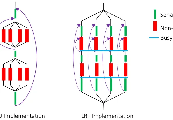
In a recent version of DA-MDS we have verified these two effects and have provided a long-running thread (LRT) implementation over FJ. Also, by adhering to strict thread process and placement we have reduced the overheads associated with threads. The difference between LRT and FJ

(19)

[image:19.612.102.398.70.276.2]

18

Figure 3-3 Fork-Join FJ vs Long Running Thread LRT implementations

Note, LRT requires a significant amount of code change from what typical MPI+X model programs look like. Also, the programmer is responsible for implementing communication after non-trivial parallel segments, whereas in FJ the built-in constructs such as parallel for implement such synchronization. Moreover, the synchronization implementation needs to make sure that none of the threads “sleep”, that is threads would be busy-waiting rather than giving up CPU resources. By performing a Linux perf counter analysis, we find this produced a smaller number of TLB misses compared to FJ.

Even with LRT implementation, the thread and process placement has to be explicit and within NUMA boundaries to get the best performance. For example, on these 2 socket nodes, placing 1 process with 24 threads is less efficient than placing 2 processes with 1 on each node having 12 threads. It is also important to pin threads to a core. In Java, pinning threads to a core is achieved using OpenHFT’s thread affinity library [30].

The point of this experiment with threads was to show that it is possible to achieve similar

performance as processes (when process communication is through shared memory), but doing so is not straightforward and requires a considerable amount of code change.

Apart from the intra-node communication optimization, SPIDAL Java employs several other techniques to reduce costs such as Java Garbage Collection (GC), cache and memory access, and heap allocated objects. GC invocations are the so-called “stop the world” events, which require all activities within the user code to be stopped while cleaning the heap. These are expensive,

especially with these Map-Collective applications where such GC events are responsible for the Serial work

Non-trivial parallel work Busy thread synchronization

(20)

strangler effect. SPIDAL Java utilizes off-heap data structures and static allocations to keep GC activity nearly at zero. Also, this makes it possible to run with a minimum memory footprint.

Cache and memory accesses also need to be optimized in yielding high-performance. SPIDAL Java adopts some of the techniques from scientific simulations to overcome these, including blocked loops, loop ordering, and 1D arrays. It is important to note that data representations with nested data structures add a substantial overhead due to multiple indirect memory references, hence the use of 1D arrays are preferred when possible.

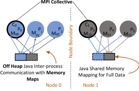
Heap allocated objects require creating temporary copies when used with native I/O operations. Therefore, SPIDAL Java utilizes off-heap memory maps to store such content. This approach is also used in loading initial large data. Memory maps not only offer off-heap allocations, but are significantly faster than the typical Java stream APIs when reading such large data. Also, for inter-node MPI communications these memory maps are more efficient than using heap allocated arrays or objects.

Figure 3-2 shows the effect of each optimization for DA-MDS as a speedup chart. The results are taken for all processes case. The base case is 48 processes run as 1x1x48, meaning 1 thread per process and 1 process per node across 48 nodes. It shows SPIDAL Java achieves around 40x speedup over 64x core count increase, while typical MPI is only able to achieve 6x speedup for the same increase in cores.

Figure 3-3 shows speedup for varying core counts for three data sizes - 100K, 200K, and 400K. These too were run as all processes because threads did not result in good performance (the tested DA-MDS did not have the LRT implementation discussed above). None of the three data sizes were small enough to have a serial base case, so the graphs use the 48 core as the base, which was run as 1x1x48. SPIDAL Java computations grow (𝑁𝑁𝑁𝑁2₎_{while communications grow}

Figure 3-4 DA-MDS speedup for 200K with different

optimization techniques

(21)

20

(𝑁𝑁𝑁𝑁), which intuitively suggests larger data sizes should yield better speedup than smaller ones and the results confirm this behavior.

In conclusion, performance results of SPIDAL Java show it scales and performs well in large PC clusters. Also, the optimizations to overcome performance challenges made it possible to run SPIDAL Java applications on much larger data sets than what was available in the past while still achieving excellent scaling results. The improved shared memory intra-node communication is pivotal to the gains in SPIDAL Java and it is the first such implementation for Java, to the best of our knowledge.

3.3. Cloudmesh Interoperability IaaS and Paas Tool leveraging DevOps

Motivation: Today’s cyberinfrastructure is complex and ever-changing. Scientists often struggle over the question of how to develop and use next generation Big Data tools and frameworks. Deployment and use of such infrastructure is complex and often beyond the expertise of data scientists.Furthermore, we have seen scientists perform unnecessary differentiations while using various IaaS platforms such as Openstack, Azure, and AWS. We also identified that the model of generating a virtual machine and using it for a long period of time is broken as security updates and other rapidly developing software render such virtual images obsolete, insecure, and outdated quickly. We need tools and frameworks that makes this easier and allow the creation and recreation of state-of-the-art tools and services used by the data scientists.

Model: Our model targets four layers in the scientific data workflow:

Phase A: IaaS deployment: Creation of virtual clusters that uses an existing HPC or IaaS system

Phase B: PaaS deployment: The platform level in which a platform is deployed or used

Phase C: Application deployment: The application deployment and development on A) and B)

Phase D: Data deployment and application execution: The execution of data analysis and experiments while using the programs developed as part of C)

(22)

3.3.1. Virtual Cluster IaaS deployment

We identified that one of the recurring tasks for data scientists is to set up a virtual cluster

containing the software needed to perform the actual activities. Through practical experience with data science students we learned that the creation of such clusters often includes sophisticated services that are beyond the capabilities of the scientist to deploy. Furthermore, subtle differences between IaaS frameworks do not allow the generality needed in the experiment on other IaaS offerings and estimate usage impact. Hence we have developed a tool called Cloudmesh that abstracts the IaaS platform and allows easy creation of virtual clusters including proper key management that often is ignored or wrongly executed by the data scientists, who may lack experience in cyberinfrastructure security. An example in Figure 3-6 illustrates the convenience of our tool. Here we demonstrate the use of persistent variables that are integrated in our Cloudmesh command line tool called cm. We can switch with a single variable between clouds, boot, assign IP addresses, and even ssh into the VMs without needing to know all the details about the cloud. An easy configuration simplifies integration of new clouds.

cm default cloud=chameleon cm vm boot

cm vm ip assign cm vm ssh

cm default cloud=kilo cm vm boot

cm vm ip assign cm vm ssh

Figure 3-6: Booting a VM is simple in Cloudmesh and uniform

While the above also allows the creation of multiple VMs, generation of a virtual cluster requires proper key management between the VMs. This is achieved through our prototype cluster command as illustrated in Figure 3-7 where we boot up 30 virtual machines and allow login between them. In addition, we implemented an inventory command that produces the necessary inventory file used, for example, by Ansible, which is part of Phase B.

cm default cloud=chameleon

cm cluster create myCluster –count=30 cm cluster ip assign # not yet implemented cm cluster setup key

cm cluster inventory

Figure 3-7: Booting a cluster of VMs is simple in Cloudmesh

(23)

22

The cluster command has been prototyped but not yet released. The interface to SDSC Comet is still in production. A tutorial will be given at XSEDE2016. A Docker interface is also under

development. A prototype to integrate VirtualBox VMs has been developed. We currently focus on Comet and NSF resources that use OpenStack.

Results: Managing VMs on different IaaS clouds is easy with Cloudmesh. Integration ofadditional clouds is possible via abstractions. The use of a savedstatein the Cloudmesh client is a

distinguishing feature from other efforts. This allows the use of defaults to simplify access to different clouds. We demonstrated use of the following clouds with Cloudmesh: FutureSystems, Chameleon Cloud, Jetstream, CloudLab, Cybera, AWS, Azure, and VirtualBox.

3.3.2. Virtual cluster PaaS, Data and Application Deployment

Once a virtual cluster is available, either as HPC, VMs, or containers, additional software services need to be installed on such a system. This can be achieved while leveraging software

configuration tools in support of DevOps such as Ansible, Chef, Pupet, Saltstack or others. In our efforts we have focused so far on Ansible as the deployment framework as it allows us to leverage a deployment methodology based on well-known security concepts and abstractions allowing a push model. Just as we can deploy such platforms, we are currently evaluating whether to use the same deployment

frameworks for application data, software and even their execution.

Status: We have developed prototype deployments for several Apache-based tools and services such as Hadoop and Spark. We have tested them on Openstack within Futuresystems and Chameleon cloud. Last semester we supported and evaluated the use of the framework and its tools in a “Big Data Open Source Software Projects Class” that had 40 teams with various projects in Big Data deployment. Based on the experience of the class we have identified that using Cloudmesh cluster will introduce much more flexibility and ease of use for the data scientists. Furthermore, we can introduce an additional abstraction layer that would allow us to integrate multiple deployment frameworks and not just

Figure 3-10: Architecture of the Cloudmesh

abstraction layers to gain access to

cyberinfrastructure systems. DevOps frameworks

are available as part of the Cloudmesh access to

them and are coordinated and choreographed with

the help of the shell, command line or a portal

(24)

focus on a single DevOps tool such as Ansible. We have made initial good progress while also using the DevOps framework for the application data and software deployment.

Access to the sophisticated cyberinfrastructure is summarized in Figure 3-8.

Summary of Cloudmesh

• Cloudmesh was downloaded 287 times in April (however since then pypi has discontinued their download information so we have no further information on downloads).

• We are presenting a tutorial at XSEDE2016 that uses Cloudmesh

• We have written a paper that was accepted at XSEDE2016 using Cloudmesh [32]

• We have identified that Cloudmesh significantly reduces startup time and effort to use multiple IaaS

• We are using the Cloudmesh principles in the current summer REU activity.

• Cloudmesh is now used to support the open science virtual cluster on Comet.

3.4. Pilot Jobs and Pilot Data Memory

Motivation: The Pilot-Abstraction offers a unified approach for application-level compute and data management across heterogeneous compute resources (e.g. HPC, cloud, Hadoop), storage

resources (e.g., local disks, cloud storage, parallel filesystems, SSD) and memory. As part of MIDAS we extended the Pilot-Abstraction to facilitate the integration of ABDS and HPC at the level of scheduling (Yarn, Slurm) and data access integrating ABDS HDFS, in-memory systems (Spark) and HPC file systems (Lustre).

With the introduction of YARN, a broader set of applications can be executed within Hadoop clusters than ever before. However, developing and deploying YARN applications potentially side-by-side with HPC applications remains a difficult task. We still lack established abstractions that are easy-to-use while still enabling the user to reason about compute and data resources across infrastructure types (i.e., Hadoop, HPC and clouds).

(25)

24

situations. Data/compute locality needs to be manually managed by the application scheduler by requesting resources at the location of a file chunk. Also, allocated resources (the so-called YARN containers) can be preempted by the scheduler.

To address these shortcomings, various frameworks that aid the development of YARN

applications have been proposed [33]. While these frameworks simplify development, they do not address concerns such as interoperability and integration of HPC/Hadoop. To facilitate the uptake of Hadoop ecosystem in an HPC context, we integrate YARN and SPARK into the RADICAL-Pilot framework, so as toprovide advanced and scalable data analysis capabilities to existing high performance applications while allowing applications to run HPC and Hadoop application parts side-by-side. These implementations are called Pilot-YARN and Pilot-SPARK.

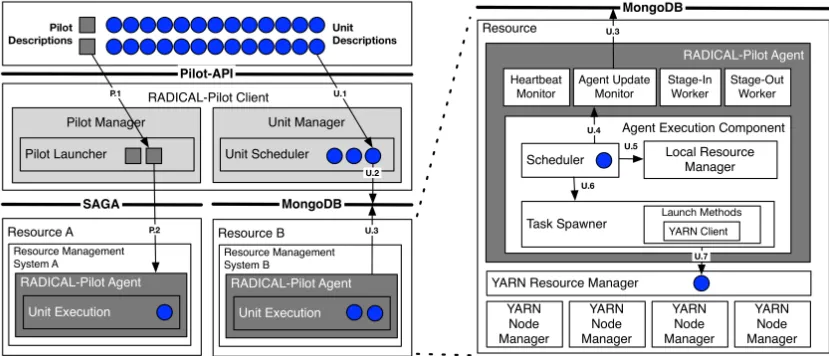
[image:25.612.103.518.405.583.2]

We extended RADICAL-Pilot to support the deployment and management of the Hadoop/Spark cluster to the resources acquired. The extension of Pilot was mainly due to the RADICAL-Pilot’s Agent which has the following components: the Agent Execution Component, the Heartbeat Monitor, Agent Update Monitor, Stage In and Stage Out workers. The integration of Hadoop/Spark was done in the agent’s execution component. Figure 3-9 shows how YARN/Spark specifics were integrated in the RADICAL-Pilot Agent.

Figure 3-9: RADICAL-Pilot YARN Architecture. All YARN/Spark specifics are encapsulated in the RADICAL-Pilot Agent

(26)

While this disk-based model is suitable for compute-bound tasks, for scalable data processing – like data transformations using the split-apply-combine pattern – more sophisticated methods are required. The usage of memory allows the efficient caching of input and intermediate data, which is essential for these algorithms.

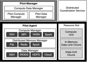
We propose Pilot-Data Memory as both an extension to Pilot-Data and as a runtime system for supporting an increasing number of iterative algorithms. Pilot-Data Memory supports application patterns, such as the split-apply-combine pattern, and iterative algorithms, as well as K-Means or optimization algorithms. It adds in-memory capabilities to Pilot-Data and makes it available via the Pilot-API. Figure 3-12 shows the architecture of Pilot-Data Memory.

An important design objective for Pilot-Data Memory is extensibility and flexibility. Pilot-Data Memory supports different memory backends: (i) file-based, (ii) memory Redis and (iii)

[image:26.612.65.436.308.569.2]

in-memory Spark. Pilot-YARN and Pilot-Spark can be used to set up the necessary Spark infrastructure on a HPC resource.

(27)

26

The different backends are supported via an adaptor service interface that specifies the

capabilities necessary for implementation by the in-memory backend; it consists of functions for allocating/de-allocating memory, loading data and executing map/reduce functions on the data. Depending on the backend, the processing function must be implemented either manually, e.g., file-based and Redis backend adaptors, or directly delegated to the processing engine as in for Spark. The Redis and file backends use the Pilot-Job framework for executing the Complete Units generated by Pilot-Data Memory. If required, the application can access the native runtime

functions via a context interface. It is important to note that Pilot-Data Memory can be easily extended to other backends, e. g. Alluxio and HDFS in-memory storage tier, which we will evaluate. Performance measurements are shown in Figure 3-11.

3.5. Architecture of Scalable Big Data Machine Learning Library

Motivation: This section establishes principles for designing parallel machine learning algorithms supporting a variety of model synchronization paradigms. It suggests a bridge between parameter server approaches and those “owner compute rule-based” distributed model parameter

[image:27.612.114.503.83.304.2]

approaches familiar in HPC.

Figure 3-13: KMeans Pilot-Data: Running KMeans on Different Pilot-Data Backends. The iterative KMeans

(28)

There is a vast amount of literature on distributed machine learning and data analytics, much of it continuing a long tradition of developing special ways to speed up or parallelize individual

algorithms or applications. However, specialized implementation rarely leads to wide-spread deployment since it yields no generalization of parallelization techniques. Thus the focus of our work [19] is to develop a general and exact parallelization technique for a large class of machine learning algorithms. It aims to provide the software building blocks (kernels) that are portable to manycore (and GPU) architectures, as we migrate from the multicore to manycore era.

We define the process for parallelization of machine learning algorithms as shown in Figure 3-12: the first step is to choose an algorithm for a given big data analysis problem. It may occur that there are multiple solutions to the same problem. An implementation is often optimized for a selected algorithm. Such a tightly coupled cycle (ref. top rectangle of Figure 3-12) works well for a specific application but becomes difficult to sustain due to diverse choices as well as changes of technology at algorithm, system and hardware levels. This motivates us to investigate the fundamental issue of

computation andparallelization abstractions

that are effective for a set of domain problems.

We propose a systematic approach with

categorizations based on “Computation Model”, which effectively expresses kernel computation characteristics and synchronization or communication mechanisms. The separation of

Computation Model, Abstraction and Implementation details allows us to adapt the variants and make the optimization easier for parallel and distributed machine learning algorithms.

Programming interface in particular provides APIs to application users.

• Computation Model

High level description of the parallel algorithm, not associating with any execution environment.

• Abstraction

Mid-level description of the parallelization, associating with a programming framework or Machine Learning

Application

Machine Learning Algorithm

Computation Model Programming

Interface Implementation

Figure 3-12. A solution for big data machine

learning application includes decisions on

algorithms, computation models,

(29)

28

runtime environment and including the data abstraction/distribution, processes/threads and the operations/APIs for performing the parallelization (e.g. network and

manycore/GPU devices).

• Implementation

Low level details of implementation (e.g. language).

We further categorize parallel machine learning applications into four types of computation models (see Figure 3-13):

Computation Model A

This computation model uses a synchronized algorithm to coordinate parallel workers. In each iteration, once a worker processes a training data item, it locks related model parameters and prevents other workers from accessing them. When the related model parameters are updated, the worker unlocks the parameters. As long as workers compute and update on different model parameters, they can execute in parallel. Only one worker is allowed to access a word's model parameters at a time; therefore the model parameters used in the local computation are always the latest. In practice, this computation model is seldom applied due to the high overhead of locking.

Computation Model B

The next computation model also uses a synchronized algorithm. Each worker first takes a partition of the shared model and performs computation. Afterwards, the model partitions are shifted between workers. When all the model partitions are accessed by all the workers, an

iteration is complete. Through model rotation, each model parameter is computed and updated by only one worker at a time so that the consistency of the model is maintained.

Computation Model C

(30)

each worker first fetches all the model parameters required by local computation. When the local computation is completed, the modifications of the local model from all the workers are combined to update the model.

Computation Model D

With this model, an asynchronous algorithm employs a stale model. Each worker independently fetches the related model parameters, performs the local computation, and returns the model updates. Unlike Computation Model A, other workers are allowed to fetch or update the same model parameter independently. In contrast to Computation Model B and C, there is no synchronization barrier in this computation model.

Based on the summarized computation models, we propose a new set of model-centric abstractions including data abstraction and synchronization operation abstraction for parallel machine learning applications as a part of the MapCollective model. These establish parallel machine learning as the combination of training data-centric and model-centric processing. The new model-centric computation abstractions can support numerous, including but not limited to:

• Expectation-Maximization Type

o K-Means Clustering

o Collapsed Variational Bayesian for topic modeling (e.g. LDA)

• Gradient Optimization Type

o Stochastic Gradient Descent and Cyclic Coordinate Descent for classification (e.g. SVM and

Logistic Regression), regression (e.g. LASSO), collaborative filtering (e.g. Matrix Factorization)

• Markov Chain Monte Carlo Type

Collapsed Gibbs Sampling for topic modeling (e.g. LDA in Section 4.2.)

3.6. Harp Programming Paradigm

Motivation: This section introduces Harp [26], whose basic idea is to abstract iterative

(31)

30

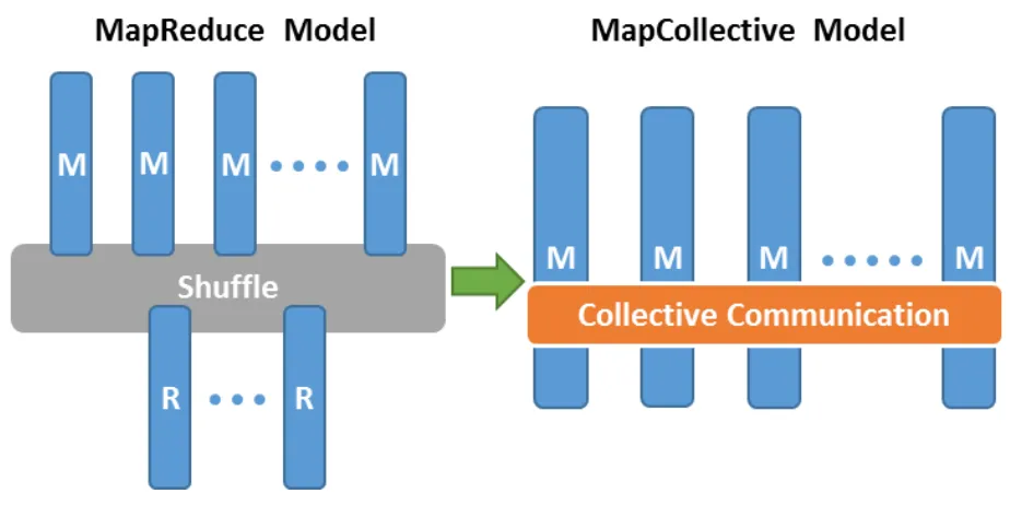
models over worker nodes and supports collective communication to bring global models to each worker node.

The Harp Programming Paradigm shown in figure 3-14, abstracts parallel applications in the

MapCollective model which is extended from the original MapReduce model. Here parallelization of an application is abstracted as parallel execution on a set of Map tasks which are synchronized with collective communication operations. While the input data is abstracted and partitioned as KeyValue pairs, the abstraction of the synchronized model data and related collective

communication operations are specially defined. These ideas are implemented in the Harp library (open source) as a Hadoop plugin. By plugging Harp into Hadoop, the MapCollective model can be expressed on top of a MapReduce framework and efficient data synchronization for a variety of machine learning applications is enabled. In addition, mapping a MapCollective model to Hadoop also enables two levels of parallelism. Since each Map task is a process where the collective communication operations are invoked and multi-thread execution is enabled for another level of parallelism.

[image:31.612.51.513.343.574.2]

The data types in Harp are abstracted in a hierarchy. Data are horizontally abstracted as arrays or key-values and constructed from basic types into partitions and tables vertically. At the lowest level, there are two basic types: arrays and objects. Based on the component type of an array, there can be byte array, int array, long array or double array. Object type is used to describe keys

(32)

and values. In the middle level, arrays and objects are wrapped as array partition and key-value partition. At the top level are tables containing multiple partitions, each with a unique partition ID. Tables on different parallel workers can be associated with each other and present one dataset. The collective communication operations are defined as redistribution or consolidation of partitions in tables.

Table 3-1: Collective Operations supported in Harp

Collective communication operations are defined on top of the data abstractions. The operations are abstracted based on the synchronization mechanisms summarized from the existing tools and many applications for learning. Currently four categories of collective communication operations are supported: (1) operations adapted from MPI: e.g. “broadcast”, “reduce”, “allgather”, and “allreduce”; (2) operations derived from MapReduce: e.g. “regroup" operation with “combine & reduce” support; (3) operations derived from graph processing tools: e.g. “send messages to vertices”; and (4) operations abstracted from machine learning applications with big models: e.g. “syncLocalWithGlobal” and “syncGlobalWithLocal”, or “rotate”.

The collective communication operations are not specific to some data abstractions. For each operation, both arrays and objects can be used. Even for graph-based communication, the

(33)

32

model to Latent Dirichlet Allocation (LDA) and show that with MapCollective abstractions the implementation can achieve better performance compared with parameter server type applications which use asynchronous communication methods.

3.7. Integration of Harp and Intel DAAL Library

Motivation: For machine learning libraries, it is obviously advantageous to reuse highly optimized kernels as software building blocks. Intel's Data Analytics Acceleration Library (DAAL) [43]

provides several core algorithms with excellent intra-node parallelism. Here we explore using Harp to invoke DAAL and thus build a distributed version of this library.

We aim to combine the advantages of Intel's DAAL for intra-node multithreading and Harp programming framework for inter-node communications. Intel optimizes a select group of data analytics and machine learning algorithm kernels on their hardware platforms, from CPUs to more recent Xeon Phi coprocessor of manycore architectures. As an extension to its highly reputable Math Kernel Library (MKL), DAAL provides high performance on its batch mode. Yet the

performance of its kernels on distributed mode relies on the communication framework chosen by the users, which motivates our effort to interface Harp with DAAL. Harp is designed to handle communication overheads within iterative applications by using collective in-memory

communication operations. Yet the implementation of local computation within the current version of Harp, which is written in multi-threading Java, is not straightforward in memory management. Thus, an integrated Harp-DAAL programming framework shall result in a significant improvement of the performance.

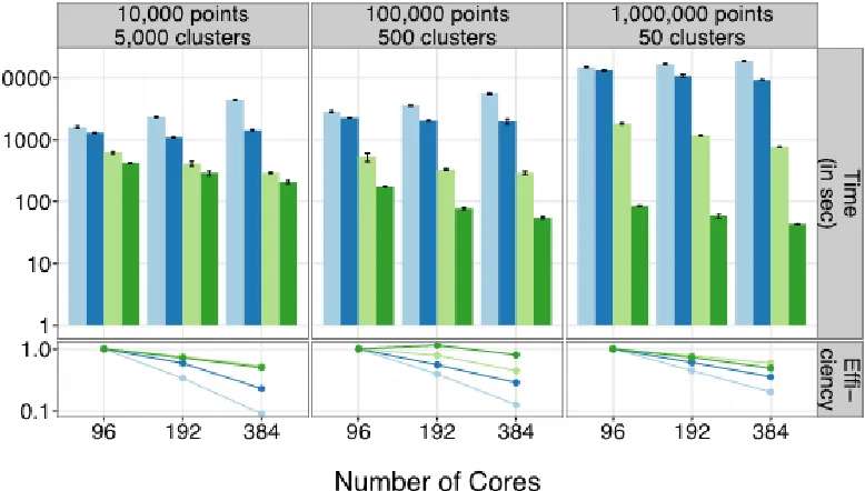
Input data has 500k points and varies centroids 1000, 10000, 100000

Input data varies points 5000, 50000, 500000 and has100k centroids

(34)

Fig. 3-15 shows a performance comparison between two implementations of K-means clustering. The experiments are done on two nodes of Haswell Xeon processor within a cluster of the

FutureSystems testbed. The K-means kernel with local computation offloaded to DAAL (red lines) achieves significantly lower execution time than the kernel implemented by Java threads.

The Harp-LDA algorithm is implemented using Java threads, while the Harp-DAAL-LDA algorithm takes advantage of the optimized native computation kernels on Intel's platform. Unlike K-means clustering, LDA has complicated irregular memory access, which requires more effort to reduce the memory data transfer overheads. Moreover, there is no LDA kernel within the current version of DAAL. We need to write the native LDA while calling the optimized MKL kernel at low levels. Our approach includes two aspects:

Data type conversion between Harp and native kernels

Harp, due to its optimization on collective communication among nodes, adopts a massive use of memory allocation in a nonconsecutive way. In contrast, DAAL and MKL allocate the data on contiguous memory chunks, which better fits the requirement of data alignment within BLAS operations. A compromise should be made between the two aspects and so we attempt to create some highly efficient data conversion methods. In order to profile the memory usage of kernels within the Harp-DAAL framework, we use Intel VTune Amplifier as a profiling tool. We also conceive a way to profile the Harp/Hadoop applications by VTune, though VTune is mainly used for profiling programs written in native languages.

Memory Optimization on Intel's Xeon Phi Knights Landing

(35)

4 SPIDAL

Algorithms

4.1. Introduction

4.2. Harp Latent Dirichlet

Allocation

4.3. SPIDAL Algorithms –

Subgraph mining

4.4. SPIDAL Algorithms –

Random Graph

Generation

4.5. SPIDAL Algorithms –

Triangle Counting

4.6. SPIDAL Algorithm –

Community Detection

4.7. SPIDAL Algorithms –

Core

4.8. SPIDAL Algorithms –

Optimization

4.9. SPIDAL - Algorithms

Polar Remote

Sensing Algorithms

4.10. SPIDAL Algorithms –

Nuclei Segmentation

for Pathology

Images

(36)

4.1. Introduction

[image:36.612.53.557.365.687.2]

In the original proposal, we identified a set of algorithms to address in SPIDAL:

Table 4-1 Status & Parallelism Abbreviations Used in Tables 4-2 to 4-4

GML Global (parallel) Machine Learning ToDo No prototype Available

PP Pleasingly Parallel (Local ML) Seq Sequential version Available

GrA Good distributed algorithm needed P-DM Distributed memory parallel algorithm

Available

GrB Graphs with runtime parallel partitioning P-ShM Shared memory parallel algorithm

Available

GrC Graphs with static parallel partitioning

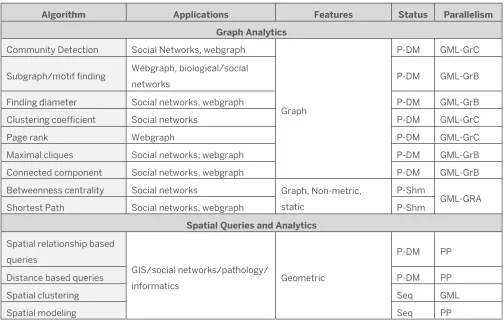
Table 4-2 Proposed SPIDAL Algorithms for Graphs and Spatial Analytics

Algorithm Applications Features Status Parallelism

Graph Analytics Community Detection Social Networks, webgraph

Graph

P-DM GML-GrC

Subgraph/motif finding Webgraph, biological/social

networks P-DM GML-GrB

Finding diameter Social networks, webgraph P-DM GML-GrB

Clustering coefficient Social networks P-DM GML-GrC

Page rank Webgraph P-DM GML-GrC

Maximal cliques Social networks, webgraph P-DM GML-GrB

Connected component Social networks, webgraph P-DM GML-GrB

Betweenness centrality Social networks Graph, Non-metric, static

P-Shm

GML-GRA

Shortest Path Social networks, webgraph P-Shm

Spatial Queries and Analytics Spatial relationship based

queries

GIS/social networks/pathology/

informatics Geometric

P-DM PP

Distance based queries P-DM PP

Spatial clustering Seq GML

(37)

[image:37.612.54.558.371.719.2]

36

Table 4-3 Proposed SPIDAL Algorithms for Image Processing and Deep Learning

Table 4-4 Proposed SPIDAL Core and Optimization Algorithms

Algorithm Applications Features Status Parallelism

DA Vector Clustering Accurate Clusters Vectors P-DM GML

DA Non-metric Clustering Accurate Clusters, Biology, Web Non metric, O(N2₎ _P-DM _GML

K-means; Bsic, Fuzzy and Elkan Fast Clustering Vectors P-DM GML

Levenberg-Marquardt Optimization Non-linear Gauss Newton, use in

MDS Least Squares P-DM GML

SMACOF Dimension Reduction DA-MDS with general weights Least Squares,

O(N2₎ P-DM GML

Vector Dimension Reduction DA-GTM and others Vectors P-DM GML

TFIDF Search Find nearest neighbors in document corpus

Bag of “words”

(image features) P-DM PP

All-pairs similarity search

Find pairs of documents with TFIDF distance below a threshold

Bag of “words”

(image features) Todo GML

Support Vector Machine (SVM) Learn and Classify Vectors Seq GML

Random Forest Learn and Classify Vectors P-DM PP

Gibbs sampling (MCMC) Solve global interference

problems Graph Todo GML

Latent Dirichlet Allocation LDA with

Gibbs sampling or Var. Bayes Topic models (Latent factors) Bag of “words” P-DM GML Singular Value Decomposition

(SVD) Dimension Reduction and PCA Vectors Seq GML

Hidden Markov Models (HMM) Global inference on sequence

models Vectors Seq PP & GML

Algorithm Applications Features Status Parallelism

Core Image Processing

Image preprocessing

Computer vision/pathology informatics

Metric Space Point sets, Neighborhood sets & Image features

P-DM PP

Object detection & segmentation P-DM PP

Image/object feature

computation P-DM PP

3D image registration Seq PP

Object matching

Geometric Todo PP

3D feature extraction Todo PP

Deep Learning

Learning Network, Stochastic Gradient Descent

Image Understanding, Language Translation, Voice Recognition, Car driving

Connections in artificial

(38)

In addition, there are community specific analytics often building on some of those in Tables 4-2 to 4-4. Table 4-2 is covered in subsections 4.3, 4.4 and 4.5. Table 4-3 is covered in subsections 4.8 to 4.10, while Table 4-4 is covered in subsections 4.2, 4.6 and 4.7.

4.2. Harp Latent Dirichlet Allocation

Motivation: Latent Dirichlet Allocation is an important algorithm that is representative of several related sophisticated latent factor (topic) determination problems. Additionally, it involves data structures and can benefit from loosening synchronization between model parameters in the different processes of a parallel algorithm. It was therefore a natural case to investigate with the Harp MIDAS technology which had been proven effective in simpler cases, especially DA-MDS, reported later under core machine learning.

The research work focuses on the computation models and the synchronization mechanisms of parallel machine learning applications using Latent Dirichlet Allocation as an example [25]. LDA is a widely used machine learning technique for Big Data analysis, including text mining, advertising, recommender systems, network analysis, and genetics. We use Collapsed Gibbs Sampling (CGS) algorithm to solve LDA. A major challenge is the scaling issue in parallelization owing to the fact that the model size is huge and parallel workers need to synchronize the model continually. We identify three important features of the model in parallel LDA CGS computation: (1) the model volume required for local computation is high; (2) the time complexity of local computation is proportional to the related model size; (3) the model size shrinks as it converges. By investigating collective and asynchronous methods of the model synchronization mechanisms, we discover that optimized collective communication can improve the model update speed, thus allowing the model to converge faster. The performance improvement derives not only from accelerated

communication but also from reduced iteration computation time as the model size shrinks during the model convergence. To foster faster model convergence, we design new collective

communication abstractions and implement two Harp-LDA applications, “lgs” and “rtt”.

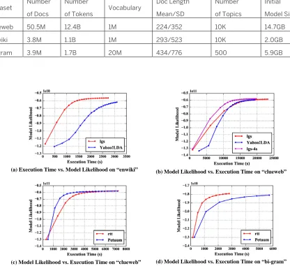
We compare our new approach with Yahoo! LDA and Petuum LDA, two leading implementations favoring asynchronous methods in the field, on a 100-node, 4000-thread Intel Haswell cluster with three different datasets (see Table 4-5). When using local-global model synchronization on

(39)

[image:39.612.93.509.135.516.2]

38

“rtt” runs 3.9 times faster compared with Petuum LDA (see Fig. 4-1d). The details of this research work are described in [14].

Table 4-5 Training Data Settings

Dataset Number of Docs

Number

of Tokens Vocabulary

Doc Length

Mean/SD

Number

of Topics

Initial

Model Size

clueweb 50.5M 12.4B 1M 224/352 10K 14.7GB

enwiki 3.8M 1.1B 1M 293/523 10K 2.0GB

bi-gram 3.9M 1.7B 20M 434/776 500 5.9GB

(a) Execution Time vs. Model Likelihood on “enwiki” _{(b) Model Likelihood vs. Execution Time on “clueweb”}

(c) Model Likelihood vs. Execution Time on “clueweb” (d) Model Likelihood vs. Execution Time on “bi-gram”

Figure 4-1. Performance comparison between “lgs” and Yahoo! LDA

and Performance comparison between “rtt” and Petuum

4.3. SPIDAL Algorithms – Subgraph mining

(40)

banks/individuals, and edges represent financial transactions, an investigator might be interested in specific transaction patterns from an individual to banks, e.g., through suspicious intermediaries to deflect attention [38]. In many bioinformatics applications, frequent subgraphs (referred to as “motifs”) in protein-protein interaction networks (PPI) have been used to characterize the

network, distinguish it from random networks and identify functional groups [39, 40].

Relational subgraph analysis, e.g. finding labeled subgraphs in a network, which are isomorphic to a template, is a key problem in many graph-related applications. It is computationally challenging for large networks and complex templates, and thus we are working on algorithms for relational subgraph analysis using Harp. We study a variety of subgraph isomorphism problems, such as: (i) counting the number of embeddings of a given labeled/unlabeled template; (ii) finding the most frequent subgraphs/motifs efficiently from a given set of candidate templates; and (iii) computing the graphlet frequency distribution.

By plugging Harp into Hadoop, we can express the MapCollective model in a MapReduce

framework and enable efficient in-memory collective communication between map tasks. It stores the intermediate data (or model data) on all nodes, each node with a different partition.

An algorithm for subgraph analysis using Hadoop, called Sahad, is given in [41], which is based on a color-coding scheme [42].

Network No. Of Nodes (in million)

No. Of Edges (in million)

Size (MB)

Web-google 0.9 4.3 65

Miami 2.1 51.2 740

Datanet: CIF21 DIBBs: Middleware and High Performance Analytics Libraries for Scalable Data Science NSF14 43054 Progress Report