Machine Learning for Parameter Auto tuning in Molecular Dynamics Simulations: Efficient Dynamics of Ions near Polarizable Nanoparticles

Auto-tuning in Molecular Dynamics

Simulations: Efficient Dynamics of Ions

near Polarizable Nanoparticles

Reprints and permission:

sagepub.co.uk/journalsPermissions.nav DOI: 10.1177/ToBeAssigned www.sagepub.com/

JCS Kadupitiya

_{, Geoffrey C. Fox}

_{and Vikram Jadhao}

Abstract

Simulating the dynamics of ions near polarizable nanoparticles (NPs) is extremely challenging due to the need to solve the Poisson equation at every simulation timestep. Recently, a molecular dynamics (MD) method based on a dynamical optimization framework bypassed this obstacle by representing the polarization charge density as virtual dynamic variables, and evolving them in parallel with the physical dynamics of ions. We highlight the computational gains accessible with the integration of machine learning (ML) methods for parameter prediction in MD simulations by demonstrating how they were realized in MD simulations of ions near polarizable NPs. An artificial neural network based regression model was integrated with MD and predicted the optimal simulation timestep and critical parameters characterizing the virtual system on-the-fly with94.3%success. The integration of ML method with hybrid OpenMP/MPI parallelized MD simulations generated accurate dynamics of thousands of ions in the presence of polarizable NPs for over10million steps (with a maximum simulated physical time over30ns) while reducing the computational time from thousands of hours to tens of hours yielding a maximum speedup of≈3from ML-only acceleration and a maximum overall speedup of≈600from ML-hybrid Open/MPI combined method. Extraction of ionic structure in concentrated electrolytes near oil-water emulsions demonstrates the success of the method. The approach can be generalized to select optimal parameters in other molecular dynamics applications and energy minimization problems.

Keywords

Machine Learning, Nanoscale Simulations, Energy Minimization, Hybrid MPI/OpenMP, Parallel Computing, Auto-tuning

1

Introduction

Many biological and synthetic nanoparticle (NP) systems are polarized in the presence of electric fields generated by surrounding ions and other macromolecular charged

species (Levin 2005; Clapham 2007; Abrua et al. 2008).

Examples include proteins and DNA in an aqueous cel-lular medium, emulsions where oil and water are parti-tioned, and gold NPs dispersed in water. Accurate knowl-edge of ionic structure near the surface of these NPs enables the understanding of many nanoscale phenomena associated with these materials such as protein

confor-mational changes (Honig and Nicholls 1995), DNA

pre-cipitation (Raspaud et al. 1998), spontaneous

emulsifica-tion (Sacanna et al. 2007), and nanoparticle self-assembly

(Levin 2005). Extracting this structure by simulating the dynamics of ions in the presence of polarizable NPs using coarse-grained models is challenging due to the need to compute polarization (induced) charges in order to

propa-gate the ion configuration (Allen et al. 2001; Marchi et al.

2001;dos Santos et al. 2011;Fahrenberger et al. 2014). This computation typically involves solving the second-order Poisson differential equation in 3-dimensional space at each simulation timestep, making the use of conventional nanoscale simulation methods very time consuming and inefficient. Because of these computational challenges, the problem of extracting ionic structure near polarizable NPs

has been a subject of intense research (Marchi et al. 2001;

Boda et al. 2004; Allen et al. 2001; dos Santos et al. 2011;

Jadhao et al. 2012,2013;Fahrenberger et al. 2014;Gan et al. 2015;dos Santos and Netz 2018).

The problem is often re-casted in terms of energy minimization for which different candidate functionals and associated minimization methods have been proposed (Marchi et al. 2001; Boda et al. 2004; Allen et al. 2001). Among these techniques, a molecular dynamics (MD) method based on the dynamical optimization of an energy functional enabled the replacement of the expensive solution of the Poisson equation at each simulation step with an on-the-fly computation of surface polarization charges (Jadhao et al. 2012,2013;Jing et al. 2015). The main focus of this paper is to highlight the computational gains accessible by integrating machine learning (ML) methods for parameter auto-tuning in MD simulations by demonstrating how these gains were realized in the MD simulations of ions near polarizable NPs based on the aforementioned dynamical optimization framework.

1_{Intelligent Systems Engineering, Indiana University, 2805 E. 10th}

Street, Bloomington, Indiana 47408, USA

Corresponding author:

Vikram Jadhao, Intelligent Systems Engineering, Indiana University, 2805 E. 10th Street, Bloomington, Indiana 47408, USA

In the dynamical optimization framework, inspired by the Car-Parrinello method for simulating ion-electron systems (Car and Parrinello 1985), an energy functional of the polarization charge density was dynamically optimized resulting in the physical dynamics of ions in parallel with the update of the virtual variables characterizing the polarization (induced) charge density. The virtual system was evolved in a manner that kept the induced charges close to the free-energy minimum (“ground state”) corresponding to the evolving ionic configuration. The advantages associated with the on-the-fly computation of polarization effects in conjunction with the reduction in computational costs achieved by solving for the scalar induced density variable enabled the study of electrolyte ion solutions near polarizable NPs

using this framework (Jadhao et al. 2012; Jing et al. 2015).

However, the applicability of the original method was limited by the absence of a framework that automates the process of selecting the “good” parameters characterizing the virtual system as well as the optimal simulation timestep. These quantities determine the stability, accuracy, and overall efficiency of the dynamical optimization framework and they were found by a tedious process of trial and error that was informed by in-domain experience. Further, these parameters were selected at the start of the simulation and held fixed throughout the simulation, to often relatively conservative values, in order to ensure the long-time stability of the dynamics of ions.

Recent years have witnessed a remarkable growth in the use of ML to enhance computational methods aimed at understanding phenomena in materials science, biology,

neuroscience, and physics (Bart´ok et al. 2017; Ch’ng et al.

2017; Balakrishnan and Puthusserypady 2005; Schoenholz 2018; Liu et al. 2017; Long et al. 2015; Ferguson 2017). ML has been applied to identify interesting parameter

spaces (Spellings and Glotzer 2018), predict parameters

(Balakrishnan and Puthusserypady 2005), update

configura-tions (Botu and Ramprasad 2015), infer assembly landscapes

(Long et al. 2015; Ferguson 2017), and classify phases of

matter (Ch’ng et al. 2017). Inspired by these recent

devel-opments, we describe an approach to integrate ML with MD methods to predict and auto-tune relevant parameters and simulation timestep. This approach is applied to the dynamical optimization framework to predict on-the-fly the virtual system parameters and simulation timestep that keep the polarization charge density close to the ground state determined by the evolving ionic configuration at all times during the simulation. The demonstration of the use of ML to predict and tune the MD simulation timestep has broad applicability. Similarly, we expect that the idea of using ML for predicting virtual system parameters can be extended to enhance the original Car-Parrinello molecular dynamics

techniques (Car and Parrinello 1985) for simulating

ion-electron systems.

The use of ML to enhance the performance of the dynamical optimization framework is demonstrated using anO(n2₎

algorithm to propagate the dynamics of ions and virtual system variables that is accelerated by implementing a hybrid OpenMP/MPI parallelization approach to reduce the computing time associated with the evaluation of the forces and energies. The target applications of the framework are systems where the effects of NP surface charge and

ion correlations typically lead to ion distributions that reach constant bulk value within a few nanometers of the NP surface such that a comprehensive study of ion densities near NP surfaces can be performed by including thousands of ions in a large simulation cell with reflective boundaries (dos Santos et al. 2011; Messina 2002; Boda et al. 2004). Many synthetic and biological systems including oil-water emulsions, gold nanoparticles (1 - 10 nm in diameter), and globular proteins exhibit this scenario, and ion distributions

in these systems have been analyzed using O(n2₎

methods

that are competitive with O(nlogn) methods for these

moderately-sized systems (Allen et al. 2001; Boda et al.

2004; dos Santos et al. 2011;Messina 2002; Hatlo and Lue 2008; Jadhao et al. 2012). Further, attempts to ameliorate

this scaling via the use of Ewald sums (Deserno and Holm

1998) or multigrid methods (Sagui and Darden 2001) would

introduce more variables and parameters into the system making the assessment of the coupling of the ML-enabled parameter selection process with the simulation of ions and virtual system difficult. The use of such methods is thus avoided in this first study of developing ML-based enhancements for the treatment of polarizability effects in ionic soft-matter simulations; future work will include integrating this approach with fast Ewald solvers for incorporating long-range effects.

As we discuss later in the results section, the ML-enhanced dynamical optimization framework leads to an increase in both the efficiency and stability of the associated MD simulations, while retaining the accuracy of the unautomated, non-adaptive framework. This combination of ML and parallel computing in the context of nanoscale simulation of ions is the first of its kind and paves the way for employing the simulation framework for developing online applications for web-based platforms like nanoHUB (Klimeck et al. 2008), where the user interacts with the simulation software under limited interaction with the developer and/or in-domain expert. An application that simulates the self-assembly of ions near polarizable NPs by employing the unique features of this framework was

recently deployed on the nanoHUB cloud (Kadupitiya et al.

2018). As is evident by the use of ML in numerous

commercial platforms, scientific simulation workflow and software applications will increasingly employ an ML layer in the future. Understanding the integration of ML in scientific applications is thus critical; the work presented here contributes towards this goal.

2

Background and Related Work

2.1

Model and the Energy Functional

The problem of evaluating polarization effects in simu-lation of charged systems has been extensively explored by several research groups using different approaches (Marchi et al. 2001;dos Santos et al. 2011;Boda et al. 2004;

Tyagi et al. 2010; Barros et al. 2014; Gan and Xu 2011;

Jadhao et al. 2012; Wynveen and Bresme 2006;Allen et al.

2001). Explicit simulation of solvent (environment) and

NPs is possible (Wynveen and Bresme 2006) using advanced

computational techniques such as fast multipole methods and

local electrostatics algorithms (Rottler and Maggs 2004); the

ion dynamics at the molecular scaleBeckstein et al.(2004). However, many phenomena can not be suitably investigated using fully atomistic models due to the prohibitively large number of degrees of freedom associated with such systems. This has led to the study of coarse-grained models that treat ions explicitly but replace the molecular structure of the solvent and the NP with continuous dielectric environments. Systems where the different material parts are adequately captured by piecewise-uniform dielectric permittivities (e.g. NP and solvent, protein and cellular medium) have attracted

particular attention (Allen et al. 2001; Boda et al. 2004;

dos Santos et al. 2011; Xu 2013; Jadhao et al. 2012,2013;

Barros and Luijten 2014;Tyagi et al. 2010). For these model systems, solving for the polarization (induced) charge den-sity reduces the computational costs because the unknown induced charge density resides only on the two-dimensional interface (boundary) between the NP and the surrounding medium. We work with such a coarse-grained model.

The dynamical optimization framework for extracting ion distributions from simulations of the coarse-grained model that treats the solvent and NP as dielectric continua is based on the true energy functional of induced charge density introduced inJadhao et al.(2012):

F_{[ω] =}1

2 Z Z

ρrGr,r′(ρr′+ Ωr′[ω]) dr′dr

−1

2 Z Z

Ωr[ω]Gr,r′(ωr′−Ωr′[ω]) dr′dr, (1)

where ρ and ω are the ion and induced charge densities

respectively. The functionG(r,r′) =|r−r′|−1is the bare

Green’s function andΩis given by

Ωr[ω] =∇ ·

χr∇ Z

(ρr′+ωr′) dr′

, (2)

where χ(r) is the dielectric susceptibility. χ(r) is related

to the spatially-varying dielectric permittivity ǫ(r) via the

relationǫ= 1 + 4πχ. The minimization ofF_{[ω]leads to the}

equation:

ω= Ω. (3)

Solving this equation is equivalent to solving the Poisson equation; its solution produces the correct induced density (Jadhao et al. 2012,2013). At its minimum,F_{[ω]evaluates}

to the true electrostatic energy of the system. These features

allowF_{[ω]to be optimized dynamically as the ions move to}

their new positions.

The functionalF_{[ω]can be transformed into a functional}

of only the surface (two-dimensional) induced charge density for the case of polarizable NP in a solvent where the NP and the solvent are modeled as materials of different,

but uniform, permittivities (Jadhao et al. 2012, 2013). The

discretized form of this transformed functional obtained by

meshing the NP surface intoM finite elements is given as:

F_{[{ωk}] =} 1

2 N X

i=1

N X

j6=i

qiK

◦◦

r_i,r_jqj+ 1 2

N X

i=1

M X

k=1 qiK

◦•

r_i,s_kωkak

+1 2

M X

k=1

M X

l=1 ωkK

••

s_k,s_lωlakal, (4)

whereωk,s_k, anda_k are, respectively, the induced charge,

position vector, and area associated with the kth finite

element. Here, N is the total number of ions, and qi

and r_i are the charge and position vector of the ith ion

respectively. The termsK◦◦,K◦•, andK•• in (4) are the effective potentials of interaction between two ions, between an ion and an induced charge, and between two induced charges; explicit expressions of these functions can be found in the

original papers (Jadhao et al. 2012, 2013). F_{[{ωk}] can}

be minimized dynamically using MD methods that treat the induced charges on the surface as dynamic variables; the details of this dynamical optimization framework are

provided in Section3.

2.2

Nanoscale Simulation of Ions near

Polarizable Materials

We review the techniques of computing ion distributions in systems described by the coarse-grained model of ions near NP-solvent dielectric interface separating NP and solvent that exhibit different (but uniform) dielectric response (permittivities) (Boda et al. 2004;Tyagi et al. 2010;

Allen et al. 2001; Barros et al. 2014; Jadhao et al. 2012,

2013;Jing et al. 2015), focusing on methods that are broadly applicable and are not limited by the choice of NP geometry or dielectric permittivity profile.

We first outline the methods based on variational approaches to the problem of evaluating the polarization effects as these techniques are most closely related to the work presented here. In this approach, one transforms the original problem of solving the Poisson differential equation into an optimization problem. A variety of functionals employing various electrostatic quantities as field variables have been proposed to formulate the variational optimization

problem (Jackson 1999; Marcus 1956; Felderhof 1977;

Reiner and Radke 1990;York and Karplus 1999;Allen et al. 2001;Attard 2003;Rottler and Maggs 2004;Lipparini et al. 2010; Villasenor and Buneman 1992; Nakano et al. 1994).

Allen et al.(2001) performed an explicit (static) optimization of a functional of the induced surface charge density

ω(s) at each MD step to solve the Poisson equation and

propagate ions. Marchi et al. (2001) worked with a true

energy functional of the polarization vector and implemented a dynamical optimization framework to propagate ion dynamics in parallel with the evaluation of polarization vector fields. However, the choice of the polarization vector as the variable field needed a three-dimensional specification leading to increased computational costs that can be avoided by choosingω(s)as the variable to solve for.

Another class of methods for computing ω(s) involves

transforming the problem into a matrix formulation; examples include the induced charge computation (ICC)

methods (Boda et al. 2004), which use matrix inversions

to solve for ω(s). Evaluating matrix inversion involves

O(M3₎

calculations where M is the number of surface

mesh elements. Techniques to improve upon this scaling

have been subsequently developed (Tyagi et al. 2010).

Alternatively, iterative methods to solve the matrix equation

have been proposed (Barros and Luijten 2014). In particular,

the generalized minimum residual method solves the matrix equation without explicitly constructing the inverse matrix

and yields a converged result for ω(s) at each simulation

The evaluation ofω(s)in all the above approaches needs the ionic configuration to be static and requires considerable computational effort, whether in the form of matrix inversions or convergence of the iterative optimization steps, at each simulation step to guarantee the overall stability of

the simulation. In Section 3, we present the details of a

recently developed dynamical optimization framework that

enables the simultaneous (on-the-fly) updates ofω(s)and the

ionic configuration in the same simulation step.

2.3

Parameter Prediction using Machine

Learning

Machine Learning (ML) abstractions for parameter predic-tion and tuning have been extensively employed in the performance enhancement of bigdata or deep learning

frame-works. Denil et al. (2013) used ANN and convolutional

deep learning NN to predict the parameters found in image classification tasks. The ANN was able to obtain an

accu-racy of 95%. Yigitbasi et al. (2013) employed ML-based

auto-tuning for diverse MapReduce applications and cluster configurations in Hadoop framework. Their work showed that support vector regression exhibits good accuracy while being computationally efficient for performance modeling of MapReduce applications.

ML methods have been increasingly employed in predict-ing parameters and classifypredict-ing properties associated with

physical systems (Spellings and Glotzer 2018; Schoenholz

2018; Liu et al. 2017; Morningstar and Melko 2017;

Ch’ng et al. 2017;Behler 2016;Botu and Ramprasad 2015;

Long et al. 2015; Ferguson 2017). Spellings and Glotzer

(2018) applied a simple feedforward artificial neural network

(ANN) to discover interesting areas of parameter space corresponding to crystal formation in the self-assembly of

colloidal building blocks.Balakrishnan and Puthusserypady

(2005) proposed a fast and simple prediction method for

two class Brain-Computer Interface (BCI) simulations using ANN and identified this method as the best ML approach for brain image classification.

In addition to classification based approaches, regression based prediction schemes have been employed in different

domain areas (Eng et al. 2014; Kazemi and Sullivan

2014; Cherkassky and Ma 2004; Chen and Yu 2014;

Balachandran et al. 2016; Quan et al. 2014; Yadav et al. 2016). Eng et al. (2014) used random forest regression algorithm to predict host tropism of influenza A virus

proteins with an accuracy above 96%. Similarly, ensemble

of regression trees were employed to perform face alignment for real-time applications (in one millisecond) by

Kazemi and Sullivan(2014). Support vector machine based regression (SVR) has been used for wind speed prediction by Chen and Yu (2014). Balachandran et al. (2016) have also used SVR to create an adaptive ML model to aid the design of a new materials with desired elastic properties and enhanced long-term performance using minimum number of iterations. ANN based regression has been studied by

Quan et al. (2014) to yield short term load prediction of electrical power systems based on wind power forecasting.

Yadav et al. (2016) have employed ANN based regression for forecasting solar radiation.

Recent research has also focused on exploring ML based approaches to generate trajectories (configurations) in MD and Monte Carlo simulations in order to enhance the

performance of the respective methods.Botu and Ramprasad

(2015) employed kernel ridge regression (KRR) to accelerate

the ab initio MD method for nuclei-electron systems by learning the selection of probable configurations in MD

simulations (Botu and Ramprasad 2015). (Liu et al. 2017)

employed an ANN to select efficient updates for Monte Carlo simulations of classical Ising spin models.

These explorations have inspired us to use ML to predict virtual system parameters and design an adaptive framework that updates the simulation timestep and auto-tunes the virtual parameters characterizing the dynamics of ions near polarizable NPs to yield a more stable and efficient MD simulation. Related work in the area of adapting timestep in a simulation has largely focused on using analytical approaches to multiple time step integration (Luehr et al. 2014;Tuckerman et al. 1992). Recent work has also focused on adaptive ensemble simulations to enhance the computational efficiency of biomolecular simulations

Kasson and Jha (2018). We also note that the development of autotuning technology for high-performance applications, which involves automatic generation of a search space of possible kernels for a computational task to identify the best possible kernel, has been extensively explored to reduce execution time and enhance programmer productivity (Whaley and Dongarra 1998), with recent work involving the use of ML-based approaches for identifying the search

space (Balaprakash et al. 2018). In Section 4, we describe

the results of our experiments with different regression-based ML models to identify and tune optimal virtual parameters for the dynamical optimization framework.

3

Dynamical Optimization Framework for

Simulating Ions near Polarizable NPs

In this section, we provide the details of the dynamical optimization framework for simulating ions in the presence of polarizable NPs. This framework uses Car-Parrinello

molecular dynamics (CPMD) technique (Car and Parrinello

1985; Fois et al. 1993) to dynamically optimize an energy functional of the polarization charge density which results in the propagation of the ionic configuration in tandem with

an accurate update of the polarization charges (Jadhao et al.

2012, 2013). These details will help clarify the use of the

ML-based enhancement strategies outlined in Section4.

3.1

Extended Lagrangian, Equations of

Motion and CPMD Simulation

To implement the dynamical optimization of F_[{ωk}],

the induced charges {ωk} are treated as dynamic virtual

variables. A fictitious kinetic energy is associated with this virtual system:

K ₌

M X

k=1

1 2µkω˙

2

k, (5)

where µk is the mass of thekth virtual variable (ωk). The

extended Lagrangian L with F_{[{ωk}] as its electrostatic}

additional term:

L=K ₊

N X

i=1

1 2mir˙

2

i −F[{ωk}]−H[{r_i}]. (6)

In (6), the second term is the usual total kinetic energy

associated with N ions (physical system), with mi being

the mass of the ith

ion. The final term contains a set of Lennard-Jones potentials to model the ion-ion and ion-NP steric interactions. Note thatF_{[{ωk}] ≡}F_[{ωk},{r_i}] is also a function of the set of ion positions{r_i}.

The Lagrangian L yields the following Euler-Lagrange

equations of motion:

mi¨r_i=−∇r_iF[{ωk},{ri}], (7)

µkω¨k =−∇ωkF[{ωk},{ri}], (8)

for the ith

ion and the kth

induced charge, respectively. These equations are used to evolve the induced charge

configurationon the flyusing the CPMD method. Following

(7), each ion is moved by the force−∇r_iF[{ωk};ri]in a

timestep∆during which each induced charge is updated via

theforce−∇ωkF[{ωk};ri]following (8). To simulate the

behavior of the ions at temperatureT, the extended system

of ions and the virtual variables is coupled to a set of Nos´ e-Hoover thermostats (this coupling modifies the equations of

motion (7) and (8) similar to a canonical MD routine). This

two-temperature approach is a standard feature of CPMD (Sprik 1991; Bl¨ochl and Parrinello 1992; Fois et al. 1993).

The ions couple to a thermostat at temperatureT, while the

virtual system is coupled to one atTv.

Velocity-Verlet algorithm is used to generate the dynamics of the extended system. The dynamics is associated with a conserved quantity, the total energy of the extended system,

that can be derived from the LagrangianL:

E ₌

N X

i=1

1 2mir˙

2

i +K +F[{ωk}] +H[r_i] +T +T_v. (9)

Here, T and Tv are the energy terms associated with the

thermostats controlling the temperature of the physical and

virtual systems respectively. The extended energy andK _are

monitored at periodic intervals during a CPMD simulation to assess the stability and accuracy of the simulation.

Virtual masses µk are chosen to be proportional to the

areas of the mesh points. The value of the proportionality

constantµdepends on the attributes of the physical system

(e.g., NP charge, dielectric profile, ion valencies) as well

as the simulation timestep ∆. The parameters Tv and µ

are optimized to ensure the stability and accuracy of the

simulation (see Section3.3); further technical details of the

method can be found inJadhao et al.(2012).

3.2

OpenMP/MPI Hybrid Parallelization

A system with N ions near an unpolarizable NP surface

effectively translates into a system with M additional

dynamical variables in the case of a polarizable NP within the dynamical optimization framework. Due to the long-range nature of the electrostatic interaction, the

associated computational costs scale roughly as O((N+

M)2

), with a prefactor that can be large owing to the

complexity of the terms involved in the expressions for forces derived fromF_{[{ωk}]. Indeed, performance profiling}

report generated using Performance Counters for Linux (PERF) showed that the sequential program spends the

largest amount of computation time (64.33% of the total)

calculating the forces between the ions for each step of the simulation. To reduce the computing time associated with the evaluation of these forces and enhance the performance of the simulation framework, a hybrid OpenMP/MPI parallel programming model is adopted. The hybrid model has advantages over pure MPI or pure OpenMP, when cache performance is taken into consideration. This strategy provides non-uniform memory access (NUMA) traffic and

inter-node communication (Rabenseifner et al. 2009) to

support maximum access locality and minimum number of cache misses. We note that the simulations associated with the dynamical optimization framework presented in the previous publications employed the OpenMP (shared memory) parallelization model, and consequently, were

limited in their application scope (Jadhao et al. 2012,2013;

Jing et al. 2015).

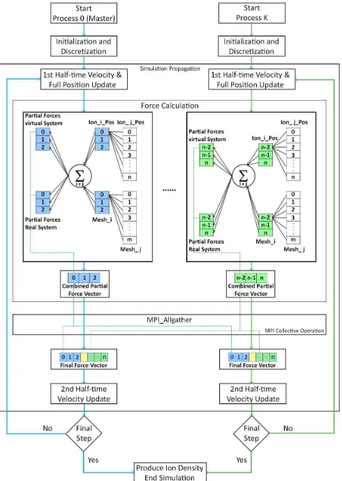
Figure 1. Distributed and shared memory parallelization

approach with MPI and OpenMP. Hybrid parallelization is implemented inside the Force Calculation block.

The hybrid masteronly model is implemented by combining the distributed memory MPI approach and

the shared memory OpenMP approach (Rabenseifner et al.

2009), and is applied to the force and energy calculation

-400 -300 -200 -100 0 100 200 300 400

0 2×106 4×106 6×106 8×106 1×107

Energy (k

B

T)

Simulation Steps

Extended Kinetic (physical) Potential Kinetic (virtual)

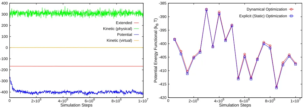
Figure 2. Energy profiles of 206 ions near a polarizable NP

(whose surface is meshed with 1082 grid points). Data is shown for≈10nanoseconds (10 million simulation steps) of

simulation time. Conservation of the extended (total) energy and≈0value for the virtual kinetic energy highlight the first key

feature of the dynamical optimization framework.

model uses one MPI process per node and OpenMP on the cores of the node, with no MPI calls inside the parallel regions. The domain decomposition is enabled under a two-level mechanism. On the MPI level, a coarse-grained domain decomposition is performed using boundary

conditions as explained in Fig. 1. The second level of

domain decomposition is achieved through OpenMP loop level parallelization inside each MPI process.

3.3

Key Framework Features

We identify two key features of the dynamical optimization framework that encode the accuracy and stability of the simulation, and guide the process of designing the ML-based

enhancement strategies presented in Section4. The first key

feature is the conservation of the extended energyE_{, given}

by Eq. (9), and the approximate conservation of the energy

of the physical system that is captured by demanding that the kinetic energy of the virtual system nearly vanishes:

K _{≈0. (10)}

In other words, the framework ensures that the physical system remains unaffected as much as possible by the presence of virtual system.

The energy profiles of a typical, successful CPMD simulation of ions near a polarizable, spherical NP at room

temperature are shown in Fig.2: the extended energyE _is

constant and the total fictitious kinetic energy stays stable

and close to 0 throughout the entire simulation run (for≈10

ns). In practice, this feature is incorporated in the simulation

by appropriately choosing values of simulation timestep∆,

virtual variable massµ, and the virtual system temperature

Tv ≪T (Tv≈0). These parameters are selected to control

large, abrupt rise in the kinetic energy associated with the virtual system as the simulation progresses.

This feature is encoded in the quantityRwhich measures

the ratio of the fluctuations in E _{and the fluctuations in}

the kinetic energy of the physical system. R determines

the stability and accuracy of the simulation. For good

-420 -415 -410 -405 -400 -395 -390 -385

0 2×106 4×106 6×106 8×106 1×107

Potential Energy Functional (k

B

T)

Simulation Steps

Dynamical Optimization Explicit (Static) Optimization

Figure 3. Comparison of the functional optimized dynamically

(circles) and the functional optimized at regular intervals keeping the ionic configuration static during the optimization process (squares). Results are shown for the same system as in Fig.2. The matching of the two functionals illustrates the second key feature of the framework: the accurate tracking of the induced charge density.

energy conservation (constant E_{), it is demanded that the}

simulations satisfy the condition R <0.05 as noted in

the literature (Marchi et al. 2001). The latter inequality

implicitly satisfies the requirement that K _{is kept close to}

the value dictated by the low temperatureTv.

The second important feature considers the effectiveness of the framework to reproduce the induced charge distribution accurately at each simulation time step. At regular intervals during the course of the simulation, the ion coordinates and induced charge densities on the NP surface are stored. Then, an ordinary (static) minimization

of the functional F _{is carried out to explicitly determine}

the (numerically) exact induced density. The tracking of the induced density distributions on the NP surface can

be assessed by evaluating the matching of F _optimized

on the fly with the electrostatic energy value obtained by

optimizing the functional explicitly; Fig.3. This functional

matching is the second key feature. In practice, we compute

the functional deviation, fd, which measures the average

difference between the dynamically optimized functional

F _{and the energy functional obtained via direct (static)}

minimization. To pass the test of stability and accuracy, we enforce|fd|<1%.

Randfdare central to the success of the simulations based

on this framework and determine the associated “good”

virtual system parameters µ and Tv. In general, higher µ

leads to better energy conservation and lower R, while

lower Tv keeps the virtual system from excessive heating

and generates lower fd. Having just these two features

biases the prediction ofµ(Tv) towards higher (lower) values

for a system of ions characterized with a generic input

parameter pattern. Very high values of µ and/or very low

values ofTvcan affect the overall stability of the simulation

the stability of the simulation and bias the selection of the virtual parameters towards those picked by a domain

expert, another quantity, Rv is introduced. Rv is the ratio

of the fluctuations inE _{and the fluctuations in}K_{. Lower}

Rv implies that fluctuations in K (that can arise from

lower virtual mass µ or higher Tv) are sufficiently strong

to endow the virtual system with the necessary dynamics

to adapt to the evolving ionic system. Unlike R and fd

that exhibit universal bounds informed by the physical

dynamics of ions, the bound onRv depends on the set of

systems investigated, and is informed largely by past domain experience. For counterion-only systems used as training

set for the ML-based methods,Rv<0.15 is enforced. For

systems characterized with electrolytes that are expected to exhibit a greater number of ions (with both positive and

negative valencies),Rvcan assume larger values depending

on the salt concentration.

Quantities R, fd, and Rv determine the choice of

the optimal virtual parameters. However, these quantities and the success of the simulation depend critically on

another important parameter: the simulation timestep ∆.

The simulation timestep in the CPMD-based dynamical optimization framework depends on both the physical and

virtual system parameters, the latter being unknowna priori.

Conversely, the optimal values of virtual parameters (µ,Tv)

that ensure a long-time stable simulation are dependent on

∆. This complicates the process for choosing a reliable, yet

efficient, value for∆,µ, andTv and one typically chooses

a conservative ∆ that is smaller than the value used in

conventional MD simulations (∆≈1−5femtoseconds for

an MD simulation of monovalent electrolyte ions in water at room temperature).

4

ML-based Enhancement of the

Dynamical Optimization Framework

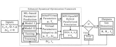
Figure 4. System overview of the enhanced dynamical

optimization framework.

We now describe an ML-based procedure to increase the efficiency and improve the stability of the dynamical optimization framework while retaining the simulation accuracy. We present an ML technique that uses the

aforementioned key features encoded in quantities R, fd,

and Rv to enhance the performance of the dynamical

optimization framework by 1) predicting and auto-tuning the

optimal virtual parameters µ and Tv, and 2) adapting the

timestep to the largest allowable value during the simulation. The ML technique is combined with MPI/OpenMP Hybrid

parallel programming model, described in Section3, to carry

out the simulation.

Figure4shows the overview of the enhanced framework.

ML-based parameter prediction was implemented using two

ML models (ML model I and II). First, the ion and NP

model attributes, as well as the initial timestep ∆ = ∆t0,

were fed to ML model I to predict the initial virtual system

parameters µ and Tv. The predicted parameters and ∆t0

were used to start the simulation that was parallelized using the MPI/OpenMP hybrid programming model. At

intermediate times tn during the simulation, ML model II

was used to predict the new timestep∆tn+1and associated

virtual parameters that continue the simulation for the subsequent time block(tn, tn+1). The ion distributions near the polarizable NP were sampled during the simulation run and the ion densities were stored as simulation output. ML model II also checks if the simulation is successful up to that point in time before dynamically tuning the parameters for next iterations to come. If simulation had failed due to

imposedR,fd, andRvcriteria, program will abort and call

the error handler to display appropriate error messages. In addition, during the simulation, the quantitiesR,fd, andRv

were computed and saved as output for retraining both ML models after a set number of simulation runs are executed. For every 1000 new simulation runs, both models were retrained.

After reviewing and experimenting with many ML techniques for parameter tuning and prediction including polynomial regression, support vector regression (SVR), decision tree regression, and random forest regression

(Section 2.3 and Section 5.1), the artificial neural

network (ANN) was adopted for enhancing the dynamical

optimization framework. Figure 5 shows the details of the

ANN-based ML model II employed to predict the virtual system parameters and the adaptive timestep for simulations based on the framework; the ANN was trained to select

the largest allowable ∆ that satisfies the tests of stability

and accuracy encoded in the ML features. ML model I exhibits a similar process but is trained without the time and timestep parameters. The data preparation and preprocessing techniques, feature extraction and regression techniques as well as their validation for both models are discussed below.

4.1

Data Preparation and Preprocessing

Counterion-only systems (no added electrolyte) were considered for generating the training set. The polarization effects are expected to be strongest in these systems as added electrolyte screens the ion-NP electrostatic interactions. Further, counterion-only systems are relatively smaller and enable a broader exploration of parameter space to train the ML models. Interestingly, as we discuss later, results from counterion-only systems were employed to successfully extract and infer ionic distributions associated

with electrolyte systems for up to O(0.1)M concentration,

exhibiting the transfer learning aspects of the ML-based procedure employed.

Prior domain experience and backward elimination using the adjusted R squared was considered for creating the training data set. Using this process, 5 input parameters that significantly affect the polarization charges on the

NP surface were identified: NP permittivity ǫNP, solvent

permittivity ǫS, NP charge Q, counterion valency v, and

NP mesh size M. While the temperature of the physical

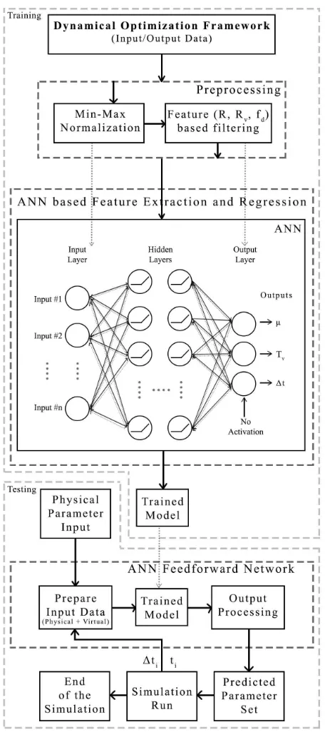
Figure 5. ML procedure (model II) for determining the parameters of the virtual system and the adaptive timestep defined in the dynamical optimization framework.

this initial study, these were considered fixed; NP diameter

was taken to be ≈7.5 times the ion diameter ( ≈

0.35 nanometers), and temperature was fixed at 298 K.

Despite the aforementioned potential for transfer learning associated with the ML procedure, additional parameters such as salt concentration and co-ion attributes should be included in the training set to predict the optimal parameters associated with the simulation of electrolyte systems; future work will explore the training with these additional input

parameters. Virtual parameter mass µ and virtual system

temperatureTvwere selected as the output parameters. Few

discrete values for each of the input/output parameters were experimented with and swept over to create and run 13600

simulations for training the ML model I. The range for different ionic system parameters were selected based on physically meaningful and experimentally-relevant values: ǫNP ∈(2,160);ǫs∈(2,160);Q∈(−20,−100);v∈1,2,3.

For the mesh size and the virtual system parameters, the range were chosen based on previous trial and error

procedure:M ∈(132,1692),µwas swept from 1 to 40 using

random discrete values to cover the range, andTvwas swept

from 0.001 to 0.005. All the simulations were performed for

≈1nanoseconds.

To support on-the-fly tuning of∆and associated selection

of µ, Tv during the simulation, ML model II was trained

with two additional parameters. Simulation time t≡tn

and timestep ∆≡∆tn+1 were added as input and output

parameters respectively to the system parameters explored

in ML model I. 20 discrete simulation time values tn ≈

0.1,0.2, . . . ,2 ns, and 4 discrete timestep values ∆ = 0.001,0.002,0.003,0.004, were swept to generate 54400 simulation configurations.

As described in Section 3.3, R, fd, and Rv encode the

key features of energy conservation and accurate tracking of the induced charges that measure the success of the dynamical optimization framework. Acceptable threshold

values 0.05, 1 percent, and 0.15 were identified for R,fd,

and Rv respectively for the range of systems included in

the training set. These quantities were treated as output features to filter the datasets to only keep the input parameter configurations resulting in successful simulation runs. From the data set for initial parameter prediction, 4530 input/output configurations were selected as successful. From the data set for adaptive timestep prediction, 15640 input/output configurations were selected. Each of these datasets were separated as training and testing using a ratio

of 0.7:0.3. Min−max normalization filter was applied to

normalize the input data in the data preprocessing stage.

4.2

Feature extraction and Regression

The ANN algorithm with two hidden layers (Fig. 5) was

implemented in Python for regression of two continuous variables in ML model I, and for regression of three continuous variables in ML model II. In both models, outputs

of the hidden layers were wrapped with therelufunction; the

latter was found to converge faster compared to the sigmoid function. No wrapping functions were used in the output layers of the algorithm.

By performing a grid search, hyper-parameters such as the number of first hidden layer units, second hidden layer units, batch size, and number of epochs were optimized to 13, 8, 25, and 150 respectively. Adam optimizer was used as the back propagation algorithm. The weights in the hidden layers and in the output layer were initialized to random values using a normal distribution at the beginning. The mean square loss function was used for error calculation in both ML models. To stop overtraining the network, a drop out mechanism for hidden layer neurons during the training time was employed. ANN implementation, training and testing was programmed

with the aid of keras and sklearn ML libraries (Chollet et al.

5

Results and Discussion

5.1

Initial Virtual Parameter Prediction

Several regression models were implemented and tested to

predict the initial virtual parametersµandTv. These models

were tested on 1359 input parameter sets comprising of values within the range for which the models were trained for. Additionally, the models were tested on 450 completely random input sets of parameters selected without any range

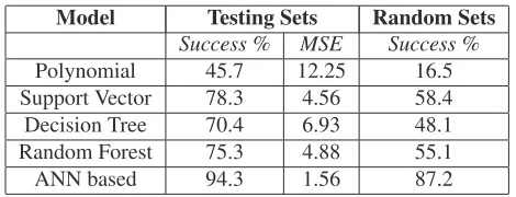
restrictions. Table1shows the success rate and mean square

error for testing data sets as well as random input data

sets. Success rate was calculated based onR, fd, andRv.

Reported mean square error (MSE) values are calculated

using k-fold cross-validation techniques withk = 10. ANN

based regression model was able to predict the initial virtual

system parameters correctly with94.3%success rate (MSE

of 1.56), outperforming other non-linear regression models

as evident from the Table1. ANN based regression model

was also able to achieve success rate of 87.2 on completely random input parameters. This ANN based regression model was adopted as ML model I.

Table 1. Comparison of the regression models for initial virtual

parameter prediction (numbers are percentages)

Model Testing Sets Random Sets

Success % MSE Success %

Polynomial 45.7 12.25 16.5

Support Vector 78.3 4.56 58.4

Decision Tree 70.4 6.93 48.1

Random Forest 75.3 4.88 55.1

ANN based 94.3 1.56 87.2

Table2shows the predictedµandTvfor selected systems

along with the quantities R, fd, and Rv that characterize

the key features of the framework, energy conservation and tracking of induced charges, that determine the accuracy and

stability of the simulation. The predictedµ andTv values

produced stable dynamics of ions near polarizable NP as

evidenced by the values ofR, Rv, and fd that lie within

allowed ranges (R <0.05,|fd|<1%,Rv<0.15).

Table 2. Predicted parameters by ML model I and simulation

accuracy and stability

Inputs Prediction Results

ǫNP,ǫS,Q, v µ Tv R fd Rv

2, 10, -60, 1 9 0.001 0.001 -0.01 0.12

2, 78.5, -30, 3 7 0.002 0.003 -0.6 0.13

50, 78.5, -60, 2 18 0.001 0.001 -0.4 0.06

80, 160, -90, 3 30 0.002 0.002 -0.7 0.09

100, 120, 30, 2 36 0.005 0.002 -0.1 0.10

5, 71, -24, 2 42 0.001 0.007 -0.6 0.13

44, 37, -114, 1 38 0.006 0.002 -0.11 0.11

30, 35, -108, 3 43 0.007 0.002 -0.12 0.05

15, 78, -102, 1 17 0.025 0.005 -0.27 0.11

We note that when the ANN was trained utilizing only

R and fd quantities, higher µ and lower Tv values were

predicted as expected from the arguments presented in

Section3.3. These virtual parameter choices are not optimal

for the stability of the simulation and will not be picked

by the experienced, in-domain expert. Inclusion of Rv as

another feature for training the model enabled the ANN to predict the virtual system parameters that were likely to enhance the stability of the simulation and be selected by a domain expert.

5.2

Auto-tuning CPMD Simulation Parameters

Similar to ML model I, ML model II employed the ANN based regression model trained with two additional

parameters: simulation timestep ∆ and timet. This model

was trained to select the largest allowed∆and auto-update

the associated optimal virtual parametersµ, Tvattnfor the

simulation during the interval (tn, tn+1) based on the ML

output featuresR, fd, andRvcomputed in the previous time

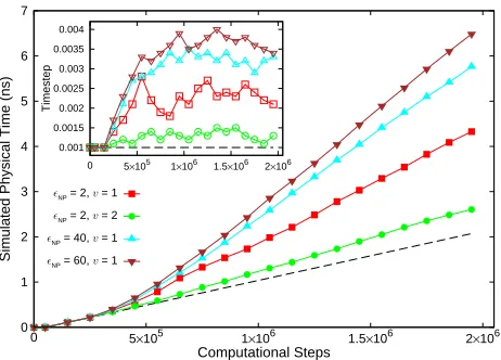
interval (tn−1, tn). Figure 6 illustrates the computational

gains resulting from the auto-tuning of∆using ML model

II for systems of counterions near a nanoparticle (NP). NPs

of different dielectric permittivity (2,40 and 60) in water

(dielectric permittivity 78.5) are considered. The effect of

varying ion valency (v= 1,2) is also probed. Other input

parameters are NP chargeQ=−100, NP mesh sizeM =

1272, andǫS= 78.5. Symbols indicate the gains associated

with the enhanced framework with adaptive timestep, dashed line is the result from the non-adaptive simulation with static timestep. Compared to the simulation with non-adaptive

∆, the auto-tuning of ∆ extended the simulation of the

ionic system to a longer physical time for the same number

of simulation steps; a speedup of 1.5−3× was observed

depending on the system configuration, also see Table3. For

the system with ǫNP= 2, v= 1, the auto-tuning yielded a

total simulated physical time of 4.5 ns compared to the 2.2

ns obtained with non-adaptive simulation. Figure 6 (inset)

shows the variation in∆as a function of the computational

steps for the same systems. The tuning of∆ changed with

the attributes of the ions and nanoparticle. Generally, longer

∆values (and associated higher speedup) were obtained for

systems exhibiting a weaker dielectric contrast.

Table3quantifies the speed by showing the performance

comparison of the aforementioned ion-NP systems for two million time steps on 4 MPI nodes each with 16 OMP threads

and a fixed walltime of ≈20 hours. ML-based adaptive

timestep tuning enabled the simulation of the system for a longer physical time under fixed compute resources and

walltime. A maximum speedup of 3.02×was achieved for

the ion-NP system defined with the input parameters:ǫNP =

60, ǫS= 78.5,Q=−100 ,v= 1 andM = 1272, without

adjusting any MPI or OpenMP parameters.

The ML-enhanced framework with adaptive timestep also

improved the overall stability of the MD simulation. Figure7

shows the key output features associated with the simulation

of the ion-NP system characterized with ǫNP= 2, v= 1

and other input parameters being the same as in Fig. 6.

Fluctuations in the output feature fd, which measures the

deviation of the on-the-fly optimized functional from the statically optimized functional, illustrate the stability of the simulation. Auto-tuning of parameters produced diminished

fluctuations infdcompared to the non-adaptive framework.

Figure7(inset) shows the variation of virtual parameter (µ)

0 1 2 3 4 5 6 7

0 5×105 1×106 1.5×106 2×106

Simulated Physical Time (ns)

Computational Steps

ǫNP = 2, v = 1

ǫNP = 2, v = 2

ǫNP = 40, v = 1

ǫNP = 60, v = 1

0.001 0.0015 0.002 0.0025 0.003 0.0035 0.004

0 5×105 _1×106 _1.5×106 _2×106

Timestep

Figure 6. Simulated physical timetassociated with the

dynamics of ions as a function of computational stepsSfor a system of counterions near a charged, polarizable NP. The legend denotes the dielectric permittivity of the NP and ion valency (ǫNP;v) associated with each system. Symbols (closed) are the results from using ML-enabled tuning of simulation timestep∆and dashed line is the result for the non-adaptive case. For a givenS, the adaptive framework yields a longer simulated physical time compared to the non-adaptive framework. (Inset) Simulation timestep (in units of≈1.09

picoseconds) for the same systems; open symbols correspond to the system denoted with the corresponding closed symbols in the outset legend. ML-enabled adaptive framework produces comparatively higher timestep values; black dashed line denotes∆ = 0.001associated with the non-adaptive case.∆ values represent the average timestep over a period of tn→tn+1.

Table 3. Performance comparison of different ion-NP systems

simulated for 2 million time steps (≈20 hrs walltime) on 4 MPI

nodes each with 16 OMP threads.

Physical System Time (ns) Speedup Stability

Non-adaptive

2, 78.5, -100, 1 2.18 1.00x 0.01552

ML-based Adaptive

2, 78.5, -100, 1 4.24 1.95x 0.00048

2, 78.5, -100, 2 2.87 1.35x 0.00088

40, 78.5, -100, 1 6.08 2.79x 0.00076

60, 78.5, -100, 1 6.57 3.02x 0.00063

definition, the non-adaptive model produced constantµ. On

the other hand, the adaptive model produced the auto-tuning

ofµwhich was correlated with the more stable dynamics (red

circles characterizingfdin the outset of Fig.7) generated by

the ML-enhanced adaptive framework. Indeed, the variance

in fd data for non-adaptive model (fd|σ2= 0.01552) was

much higher than that for adaptive model (fd|σ2 = 0.00048).

Table 3 shows the variance of fd for the same ion-NP

systems analyzed above; in all cases, variance was found to be significantly smaller (indicating higher stability) for the adaptive model compared to the non-adaptive case. This enhanced stability can be attributed to the optimal updates

of parameters µ, Tv during the intermediate times of the

simulation.

-0.6 -0.5 -0.4 -0.3 -0.2 -0.1 0 0.1

0 0.5 1 1.5 2 2.5 3 3.5 4 4.5

Key Framework Features

Simulation Time (ns)

fd (adaptive)

R (adaptive)

R_v (adaptive)

f_d (non-adaptive)

20 25 30 35 40 45

0 0.5 1 1.5 2 2.5 3 3.5 4 4.5

Virtual Parameter

µ

Adaptive Non-adaptive

Figure 7. Key output featuresR, fd, Rvas a function of

simulated physical timetfor the counterion-NP system characterized with NP chargeQ=−100, ion valencyv= 1,

NP permittivityǫNP= 2, solvent permittivityǫS= 78.5, and mesh sizeM = 1272. ML-enabled auto-tuning of∆and virtual parameters produces enhanced stability (diminished

fluctuations infd) compared to the non-adaptive case (strong

fluctuations infd). (Inset) ML-enabled auto-tuning of the virtual

parameterµfor the same system (closed circles) and fixedµfor the non-adaptive case (closed diamonds).

In addition to increasing the efficiency and stability of the simulation, the framework with ML-enabled auto-tuning of parameters (adaptive framework) retained the accuracy associated with the framework with non-adaptive timestep and virtual parameters (non-adaptive framework). The accuracy can be assessed by comparing the density profiles of the ions computed using the two approaches.

For different ǫNP values (other input parameters same as

above), the peak densities computed using simulations based on adaptive framework were found to be in agreement with those calculated using the non-adaptive framework as shown

in Figure8; data from either approach falls on the dashed line

which indicates linear correlation. Top-left inset of Figure

8 shows the variation of the counterion density (in σ−3

,

whereσ= 0.357nm is the ion diameter) as a function of the

distance from the NP (of radius 7.5σ) for the specific case

ofǫNP= 2. The density profiles extracted from the adaptive

and non-adaptive frameworks were found to be in good agreement (relative error in either distributions was found to

be≈1%). Bottom-right inset of Fig.8shows the variation of

the peak density of counterions as a function of the dielectric

permittivity ǫNP of the NP. Both approaches yield similar

peak densities. Lowering ǫNP leads to an increase in the

repulsive force on the counterions due to the induced charges on the surface of the NP, leading to the reduction in the peak density of counterions near the NP surface.

5.3

Benchmarking ML-enhanced Simulations

0.02 0.03 0.04 0.05 0.06 0.07

0.02 0.03 0.04 0.05 0.06 0.07

Peak Density (

σ

-3; Adaptive)

Peak Density (σ-3; Non-adaptive) Adaptive Non-adaptive

0 0.005 0.01 0.015 0.02 0.025

6 7 8 9 10 11 12 13 14 15

Ion Density (

σ

-3)

r (σ)

Adaptive Non-adaptive

0.02 0.03 0.04 0.05 0.06 0.07

0 10 20 30 40 50 60 70

Peak Density (

σ

-3)

ǫNP

Figure 8. Correlation between the peak densities associated

with the distribution of counterions for ion-NP systems characterized by different NP permittivityǫNP; other parameters are the same as listed in the caption of Figure7. Blue squares are values from non-adaptive simulation, red circles are results from ML-enabled adaptive simulation. (Top-left inset) Density distribution of counterions for the system withǫNP= 2; symbols are the results from adaptive model, line corresponds to the non-adaptive case. (Bottom-right inset) Peak densities from the two models as a function ofǫNP.

Dhabi x86 64 CPUs and 64 GB of RAM; each XK7 node has one AMD Opteron 16-core Interlagos x86 64 CPU, and 32 GB of RAM.

0 50 100 150 200

0 100 200 300 400 500

Speedup

Number of Processes or Threads

ML + Hybrid

ML + Hybrid

Hybrid Only

Hybrid Only 60 ions (adaptive)

60 ions (non-adaptive) 2908 ions (adaptive) 2908 ions (non-adaptive)

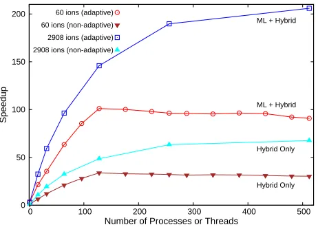
Figure 9. Strong scaling plot of the performance of

MPI/OpenMP hybrid method with and without ML-enabled adaptive timestep enhancement. Data is shown for 60 and 2908 ions; in both systems, NP is meshed with 1082 mesh points (induced charges). For both systems, ML + hybrid method outperforms hybrid-only implementation.

Figure 9 compares the strong scaling plot of the

performance of the dynamical optimization framework parallelized using the MPI/OpenMP hybrid model with and without adaptive timestep enhancement. The reported speedup is defined as the ratio of serial run-time to the time taken by the parallelized simulations (with and without

ML-enabled auto-tuning of timestep) to simulate a set tb

nanoseconds of physical system dynamics. In Figure 9,

results are shown for simulation of a system of 60 ions and 1082 mesh points as well as a larger system of 2908 ions and

1082 mesh points fortb≈2nanoseconds. The larger system

of 2908 ions is comprised of both positive and negative

ions characterized by an electrolyte concentration c≈0.2

M (with 60 counterions, 1424 positive electrolyte ions, and 1424 negative electrolyte ions). While the ML models were

not trained withcas an input parameter, simulations of the

electrolyte systems using ML-predicted timestep and optimal virtual parameters associated with counterion-only systems

were successful for over c≈0.2 M (see Section 5.4),

enabling the benchmarking of simulations of larger systems. With non-adaptive timestep, the hybrid model produced the maximum speedup of 33.80 with 128 processes (8 MPI nodes and 16 OpenMP threads inside each MPI node) for the smaller system. For the same configuration, the hybrid model with ML-enabled auto-tuning of the simulation timestep was able to achieve a maximum speedup of 101.07 with 128 processes. Thus, the runtime for the this system was reduced from 55 hours to 30 minutes (68 minutes without adaptive time-stepping). We note that the maximum speedup was calculated without considering the execution time reduction gained from the memory optimization techniques. For the hybrid model, we found that the optimal configuration of OpenMP threads is socket bound as noted in the literature (Rabenseifner et al. 2009). As a result, the number of optimal OpenMP threads in our experiment was 16 for any number of MPI processes.

When implemented to a larger system with a total number of 2908 ions and 1082 mesh points exhibiting induced charges, the combination of the hybrid methodology and the ML-based selection of adaptive timestep reduced the execution time of simulation for 2 nanoseconds from 88 days to 10.2 hours (32 hours without adaptive time-stepping) with a speedup of over 200. Clearly, the optimum number of MPI processes are proportional to the problem size when OpenMP thread affinity is set to the socket resulting in a well weak scaling system. The maximum speedup of 620.76 was obtained for 1024 processes (threads) executing a simulation

of 5816 ions and 1272 mesh points fortb ≈0.5nanoseconds.

5.4

Application: Concentrated Electrolytes

near an Oil-Water Emulsion Droplet

The ML-enhanced framework was applied to compute the distribution of monovalent electrolyte ions outside a

charged oil-in-water emulsion droplet (de Graaf et al. 2008;

Bier et al. 2008) at room temperature T = 298 K. Positive and negative ions were considered to be of the same size to simplify the system and focus on analyzing the effects of polarization charges on the density distributions. Such model systems have been considered in previous numerical studies

of electrolyte ions near polarizable nanospheres (Messina

2002;dos Santos et al. 2011;Shen et al. 2017). All ions were

modeled as Lennard-Jones (LJ) spheres of diameter σ=

0.357nm. The oil-water emulsion droplet was modeled as a

spherical, dielectric interface with surface chargeQ=−60e

and radius a= 7.5σ≈2.7 nm. The whole system of ions

and the droplet was taken to be in a large spherical simulation

cell of radius b= 40σ≈14nm. The emulsion surface and

the simulation cell boundary were modeled as spherical LJ walls. All excluded-volume interactions were modeled using

the repulsive 6-12 LJ potential withǫLJ = 1kBT and cutoff

The dielectric permittivity of oil was taken to beǫo = 2,

while water was associated withǫw= 78.5. The difference

in the polarizable properties of oil and water lead to surface polarization charges. Electrostatic interactions arising from the bare and induced charge interactions in the system were modeled using the forces originating from the functional described in Eq. (4). The oil-water dielectric interface (which can be considered as the surface of the NP) was meshed withM = 1082mesh points; higherM values were found to

yield similar densities indicating thatM = 1082was large

enough to obtain converged density profiles. In addition to

the system with no added electrolyte, systems with c≈

0.02,0.1,0.2 M were considered to analyze the effects

of changing the electrolyte concentration c on the ionic

distributions. Together with the 60 counterions (associated with the charged oil-water droplet), these concentrated

electrolytes correspond to systems with a total of350,1514,

and2968ions respectively. Simulation of the smallest system

(60 ions) assuming non-polarizable NP surface was also

performed for assessing the role of surface polarizability. It should be noted that the ML procedure was only trained

for smaller systems with counterions (c= 0, thus in the

absence of co-ions). Further the training was performed for relatively smaller computational time (up to 2 million). With the application of the ML-enhanced framework to the aforementioned systems, we are elucidating the transferability of the features learned for the smaller system

to different but related physical systems (with finite c,

presence of co-ions, and long-time dynamics). Such an extended application of the developed ML models is possible, in part, because addition of electrolytes weaken the effective interaction between counterion and oil-water surface as a result of the screened electrostatic forces.

The aforementioned attributes of the physical system supply the input parameters for the enhanced dynamical optimization framework. Following the process elucidated

in Fig.4, these system inputs were first passed to the ML

model I to predict the required virtual system parameters to kickstart the simulation. Then, ML model II was employed to auto-tune the timestep and virtual parameters during the simulation executed using the hybrid OpenMP/MPI method up to 2 million time steps. For the rest of the simulation run, ML model II was disabled and ML model I was

used. The total number of steps S were selected based

on the convergence of the density distributions; S was

system-dependent and converged results were obtained after

≈5−20 nanoseconds (14−60 hours) depending on the

electrolyte concentration.

In all simulations, regardless of system sizes and presence/absence of electrolytes, good energy conservation

was observed withR <0.05. Similarly, the induced charges

on the oil-water dielectric interface were accurately tracked by the on-the-fly optimization framework (fd <1%; inset in

Figure10shows the accurate tracking on the functional for

thec= 0.02M case). These two key features demonstrated

the success of the ML-based virtual parameter selection

process. As noted before, the bound onRvis system-size and

system-feature-dependent that is informed by prior domain

experience; for counterion-only systems,Rv<0.15 as per

the expected limit while for electrolyte systems the bound

on Rv was higher and increased with increasing c. These

0 0.2 0.4 0.6 0.8 1 1.2 1.4 1.6 1.8

2.5 3 3.5 4 4.5 5 5.5

Density of Positive Ions (M)

Distance from Emulsion Droplet Surface (nm) 0.0 M

0.02 M 0.1 M 0.2 M

-470 -460 -450 -440 -430 -420 -410 -400

2×106 4×106 6×106 8×106 1×107

Potential Energy (k

B

T)

Simulation Steps Dynamic Optimization

Static Optimization

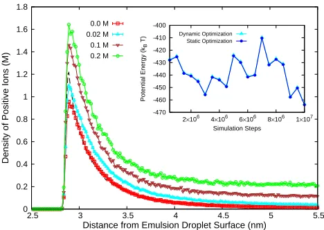
Figure 10. Ionic density profiles extracted from ML-enhanced

MD simulations based on the dynamical optimization framework. Outset shows the density of positive ions for electrolytes of concentrationc≈0.0,0.02,0.1,0.2M near

negatively-charged oil-water emulsion with dielectric permittivity of oil and water as 2 and 78.5 respectivley. Black dashed line refers to the result for the emulsion assumed to be

unpolarizable (with oil permittivity as 78.5). (Inset) Comparison of the functional optimized dynamically (diamonds) and the functional optimized at regular intervals keeping the ionic configuration static during the optimization process (circles) for c≈0_.02_{M system.}

findings demonstrated that ML models could be trained on smaller systems and applied to larger systems to obtain efficient and stable dynamics of ions in the latter case.

Figure 10shows the density profiles of the positive ions

associated with the four systems. For all concentrations, the densities reach a constant value in the bulk away from the polarizable oil-water surface (negative ion densities, not shown, also reach a constant value in the bulk). Positive ions are found to accumulate near the dielectric interface,

with the peak density increasing withc. Similarly, negative

ions are depleted near the interface due to the repulsion from the bare charge on the oil-water surface as well as the induced charge. Comparison of the no electrolyte result with the case where the surface is considered to be unpolarizable (with a permittivity equal to that of water) is also shown. The polarization charges on the surface lead to depletion of ions from the interface. Increasing concentration leads to the rise in the peak density; the overall behavior is determined by the competition between the ion-induced charge repulsion near the surface and the ion-ion electrostatic and steric correlations. The position of the peak

density remains relatively unaltered regardless of c value,

as observed previously for monovalent electrolytesMessina

(2002).

The inset in Fig.10shows the comparison of the potential

energy functional optimized dynamically with the energy obtained after optimizing at regular intervals keeping the ionic configuration static during the optimization process

for the c≈0.02 M system. The potential energy and the

associated induced charges it characterizes were accurately tracked at all times for up to 10 million time steps

(≈20 ns). The stability and accuracy evident from this