Prediction of Diesel Fired Power Plant Feeder Performance using First Order Fuzzy Time Series

Abstract— Power outages caused by factors outside the established policy will have an impact on the decline in electricity supply services and other cost related impacts. The reliability of the power plant feeder, in this case, is very important to monitor and maintain. The performance of power plant feeder can be reviewed based on the variable duration of power outage and power which fails to distribute. In this study, 1st order FTS (Fuzzy Time Series) is used to predict the feeder's performance through the predictive activity of both those variables in the actual year and the following year. The prediction results state that in 2017 there was a 20.54% decrease in performance.

Keywords— feeder, power outages, undistributed power, 1st order FTS.

I. INTRODUCTION

Reliability has been a problem for scientists and power engineers in the last decade due to costly shutdowns and downtime. Power outages caused by factors outside the established policy will have an impact on the decline in electricity supply services and other cost related impacts. Reliability is the probability that the device / system will function correctly while operating. Availability is that, the system will be able to perform its function for a certain period of time. Analyzing reliability, maintenance along with availability will be able to determine the equipment's ability to achieve a desired task [1]. Improving distribution reliability is key to improving customer reliability because distribution systems account for approximately ninety percent (90%) of all customer reliability issues. One of the most effective ways is how to perform fault detection on the distribution network through monitoring system and controlling the power system. This will improve the fault detection system and reduce response time to minimize outages and losses energy [2]. Related to the reliability of the feeder, the feeder periodically needs to be tested through various methods and techniques, including how to perform the necessary data acquisition. In general, the feeder test aims to generate actual network characteristics, including particular specificities within a particular region. This feature is called representativeness. In other words, the

Revised Manuscript Received on September 10, 2019.

Mohammad Zainuddin, Department of Electrical Engineering, State Polytechnic of Samarinda, East Kalimantan, Indonesia

(E-mail: zainuddin011062@gmail.com)

Arbain, Department of Electrical Engineering, State Polytechnic of Samarinda, East Kalimantan, Indonesia.

(E-mail: arbain4_polnes@yahoo.com)

Bustani, Department of Electrical Engineering, State Polytechnic of Samarinda, East Kalimantan, Indonesia.

(E-mail: bustani27@gmail.com)

Verra Aullia, Department of Electrical Engineering, State Polytechnic of Samarinda, East Kalimantan, Indonesia.

(E-mail: verra_aullia@yahoo.co.id)

feeder test is the representative of a certain actual networks located in certain regions or countries. Use of an important test feed is a benchmark that gives researchers an opportunity to evaluate the performance of their algorithm [3].

The power system network is expected to remain in a state of equilibrium under normal conditions and requires it to restore the system status to an acceptable condition after a disturbance, ie the voltage after disturbance is returned to a value close to the pre-disturbance situation. Voltage instability on the power system network occurs when a network failure causes a gradual and uncontrolled voltage drop. Contingencies such as lines or generator outages due to errors, increased loads, external factors, or improper operation of voltage control devices are the cause of voltage instability. If action is not taken to check for this voltage instability, this will cause a gradual decrease in system voltage and consequently a voltage collapse resulting in a partial or total system blackout [4]. Various studies have been conducted to measure the occurrence of power outages as in [5-9].

The reliability of the power plant feeder, in this case, is very important to monitor and maintain. One practical way to measure the reliability of a power plant feeder is through its performance measurement. The performance of power plant feeder can be reviewed based on the variables duration of power outage and power which fails to distribute. There are many methods and techniques to measure the performance of a power plant feeder, one of which is to predict both variables, based on historical data. There are many methods that can be used to perform predictive activities, both based on statistical methods and machine learning methods. One of them is by using First order Fuzzy Time Series (1st order FTS) as it has been done in [10-13].

This study applies the 1st order FTS to predict the outages duration and undistributed power in the following year based on historical data in the actual year. The aim of this study is to predict the performance of power plant feeder based on the predicted results of both those variables.

II. METHODS 2.1 Fuzzy Time Series

FTS (Fuzzy time series) is a data forecasting method that uses Fuzzy logic principles. Some of the FTS concepts are as follows:

Prediction of Diesel Fired Power Plant Feeder

Performance using First Order Fuzzy Time

Series

2.1.1 Fuzzy Time Series (FTS).

Given is a subset of real numbers, as the universe of discourse from the fuzzy set of

. If is collection of then is referred to

as Fuzzy Time Series on

2.1.2 Fuzzy Relation.

If there is a fuzzy relation, , such that

where “×” is an operator, then

is said to exist because of , and expressed by:

(1)

The “×” operator may be a max-min fuzzy operator, min-max, or arithmetic operator. If and

then logical relationships between and can be expressed by where is left side and is right side of fuzzy relations. The variable t denotes time.

2.1.3 First Order Fuzzy Relation.

Given is FTS. If caused by

then its fuzzy relation is expressed by:

(2)

and called n-order FTS. From Eq. (2), then it can be obtained for First Order FTS stated with Eq. (1).

2.1.3 Time-invariant FTS.

If it is assumed that is only caused by

denoted by Eq. (1) then its fuzzy relation can be expressed by the equation:

(3)

The relation R is called the 1st order relation model

of . If is independent against time “t”

(time-invariant) then for different time t1 and t2,

, then called time-invariant FTS.

2.2 Prediction using First Order FTS

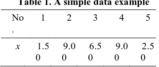
The prediction using 1st order FTS is based on Eq. (1). As an example: states that the fuzzy value of 2nd month is determined by the fuzzy value of 1st month. The following description will describe the prediction steps using the 1st order FTS with a simple data example as shown in Table 1.

Table 1. A simple data example No

.

1 2 3 4 5

x 1.5 0

9.0 0

6.5 0

9.0 0

2.5 0 2.2.1 Determining the universe of discourse, (U).

From the sample data in Table 1 obtained the minimum data = 1.50 and maximum data = 9.00. In order that the data within the interval of universe of discourse then the range of U need to be set to {0, 10}.

2.2.2 Determining the fuzzy sets.

If A is a fuzzy set and is a membership function of A, then:

(4)

is the degree of membership of x in the fuzzy set A. There are many types of membership functions (MF). In this study used trapezoidal MF which stated by:

(5)

Trapezoidal MF is shown in Fig. 1(a). Trapezoidal MF is modified to be as shown in Fig. 1(b).

a b c d

mA

X 1

a, b c, d

mA

X 1

(a) (b)

Figure 1. Trapezoidal MF

The crisp data fuzzyfication process (historical data) to output defuzzyfication is shown in Fig. 2.

Input fuzzyfication

First Order FTS Rule-based

Aggregation Output defuzzyfication Input

(crisp)

Output (crisp) Fuzzy Inference

Figure 2. Fuzzy inference using 1st order FTS There are many output defuzzyfication functions, including: centroid, bisector, mom (mean value of maximum), lom (largest value of maximum), and som (smallest value of maximum). In this study used centroid. For example from Fig. 1(a) it appears that the highest degree (mA = 1) is at the interval {b c}, so that:

(6)

2.2.3 Apply fuzzy set on universe of discourse (U).

Given U = {0, 10} then obtained: . If 5 fuzzy sets are used then obtained . The application of fuzzy set on U is shown in Fig. 3.

2.2.4 Historical dat fuzzyfication.

Referring to Table 1 and Fig. 3, for x= 6.5 are at intervals {6 8}, so that . The results of fuzzyfication process are shown in Table 2

Table 2. The results of fuzzyfication of Table 1

T x fuzzyfication center point

1 1.50 1.00

2 9.00 9.00

3 6.50 7.00

4 9.00 9.00

5 2.50 3.00

2.2.5 Building 1st order FTS relation.

Referring to Eq. (1) then obtained the relations as shown in Table 3. These relations are used as Rule-based.

Table 3. Fuzzy relations using 1st order FTS

t X fuzzyfication 1st _order FTS

Fuzzy relation

1 1.50

2 9.00

3 6.50

4 9.00

5 2.50

2.2.6 Aggregation and output defuzzyfication.

Each fuzzy relation will be implied on each data that has been fuzzyfied . All the implications for each of the fuzzyfied data then aggregated to obtain fuzzy output. As an example for . First order FTS:

. Because then the implications of

all fuzzy relationships of the crisp data are shown in Fig. 4. It is found that for only implied

in Rule 1

. The result of the aggregation is . Defuzzification of fuzzy output is obtained by using the centroid function on , so that it is obtained:

It can be seen that the predicted result of using 1st order FTS is 9 (same as crisp data).

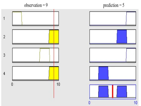
For then and 1st order FTS

is . Because then the implications of

all fuzzy relationships of the crisp data are shown in Fig. 5.

observation = 1.5 prediction = 9

Figure 4. Rule viewer for x=1.5 using Fuzzy Inference System Editor MATLAB

observation = 9 prediction = 5

Figure 5. Rule viewer for x=6.5 using Fuzzy Inference System Editor MATLAB

It is found that for implied in Rule 2 and Rule 4 . The result of the aggregation

is . Defuzzification of fuzzy output is obtained by

using the centroid function on , so that it is obtained:

It can be seen that the predicted result of using 1st order FTS is 5 (the crisp data is 6.5).

2.2.7 Validation of predicted results,

Validation of predicted results is done using MAPE (Mean Absolute Percentage Error) and RMSE (Root Mean Square Error) as expressed by:

(7)

(8)

respectively. For large data can be used MSE approach as follows:

( 9) In the same way, predicted results of all the data from Table 1 using 1st order FTS are shown in Table 4.

Table 4. The results of prediction using 1st order FTS from Table 1

No. Observat ion

prediction APE (%) SE

1 1.5 1 33.33 0.25

2 9 9 0.00 0.00

3 6.5 5 23.08 2.25

4 9 9 0.00 0.00

5 2.5 5 100.00 6.25

MAPE 31.28

MSE 1.75

Predictive results are said to be good when MAPE and MSE / BMSE are very small (close to zero). To improve predicted results until a small enough MAPE and MSE can be performed by increasing the number of fuzzy sets used.

2.3 Dataset

This study uses the dataset of the performance of diesel power plant feeder Keledang, East Kalimantan - Indonesia in 2016 as shown in Table 5. The average data calculation is using the following formula:

(10)

For standard deviation calculation is using the following formula:

(11)

Referring to Table 1, it can be seen that the average data is smaller than the standard deviation. The high deviation of data distribution can lead to significant prediction errors if existing data is used as predictive historical data. To anticipate the occurrence of a significant prediction error then the data needs to be modified by utilizing the standard deviation, expressed by:

(12)

Where is the modified data. The results of data modifications are shown in Table 6.

.Table 5. Performance of Diesel Power Plant Feeder – Keledang – East Kalimantan – Indonesia in 2016 No. Month

Outages duration (hour)

Power is not distributed (kWh)

1. January 49.13 221,960

2. February 53.40 97,661

3. March 22.88 64,171

4. April 6.75 34,418

5. May 8.40 20,234

6. June 4.98 10,887

7. July 5.53 22,210

8. August 1.78 5,563

9. September 1.45 7,238

10. October 10.47 28,618

11. November 1.22 4,989

12. December 5.47 35,376

Total 171.47 653,325

Average 14.29 54,444

Standard deviation 18.23 74,632

Table 6. The results of data modification

No.

1. 49.13 2.69 221,960 33.97 2.97

2. 53.40 2.93 97,661 30.25 2.65

3. 22.88 1.26 64,171 9.82 0.86

4. 6.75 0.37 34,418 5.27 0.46

5. 8.40 0.46 20,234 3.10 0.27

6. 4.98 0.27 10,887 1.67 0.15

7. 5.53 0.30 22,210 3.40 0.30

8. 1.78 0.10 5,563 0.85 0.07

9. 1.45 0.08 7,238 1.11 0.10

10. 10.47 0.57 28,618 4.38 0.38

11. 1.22 0.07 4,989 0.76 0.07

12. 5.47 0.30 35,376 5.41 0.47

Total 171.47 653,325

Standard

deviation 18.23

11.42

Because the data of power not distributed, in numbers tens of thousands, it needs to be converted into the percent. The results of data modification are shown in Table 6.

III. RESULTS AND DISCUSSION

3.1 The outages duration and undistributed power prediction by using 1st order FTS

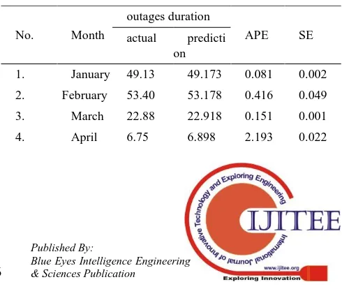
In this study, the prediction using 1st order FTS was done by using M-File program MATLAB. The first step, the prediction is done for the operating period of 2016. The prediction results are shown in Tables 7 and 8, and Fig. 6.

Table 7. The prediction results of outages duration in 2016

No. Month

outages duration

APE SE actual predicti

on

1. January 49.13 49.173 0.081 0.002

2. February 53.40 53.178 0.416 0.049

3. March 22.88 22.918 0.151 0.001

5. May 8.40 8.232 2.000 0.028

6. June 4.98 5.118 2.702 0.018

7. July 5.53 5.563 0.536 0.001

8. August 1.78 2.002 12.262 0.048

9. September 1.45 1.558 7.448 0.012

10. October 10.47 10.458 0.115 0.000

11. November 1.22 1.113 8.521 0.011

12. December 5.47 5.563 1.700 0.009

Average 14.29 14.31

MAPE 3.177

MSE 0.017

The number of fuzzy set 120

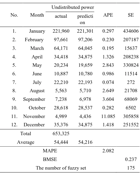
Table 8. The prediction results of undistributed power in 2016

No. Month

Undistributed power

APE SE actual predicti

on

1. January 221,960 221,301 0.297 434606

2. February 97,661 97,206 0.230 207187

3. March 64,171 64,045 0.195 15637

4. April 34,418 34,875 1.326 208238

5. May 20,234 19,659 2.843 330824

6. June 10,887 10,780 0.986 11514

7. July 22,210 22,193 0.074 272

8. August 5,563 5,710 2.649 21708

9. September 7,238 6,978 3.604 68069

10. October 28,618 28,537 0.282 6502

11. November 4,989 4,436 11.085 305858

12. December 35,376 34,875 1.418 251552

Total 653,325

Average 54,444 54,216

MAPE 2.082

BMSE 0.237

The number of fuzzy set 175

Figure 6. Graph of predicted outages duration and undistributed power in 2016

Referring to Tables 7 and 8, both MAPE and MSE/BMSE for these predictions can be considered small enough. In this case it can be said that 1st order FTS is good enough to describe the pattern of historical data.

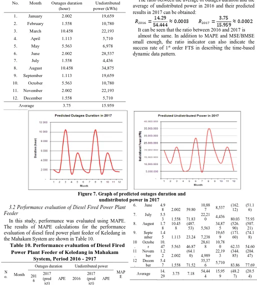
Table 9. The prediction results in 2017 No. Month Outages duration

(hour)

Undistributed power (kWh)

1. January 2.002 19,659

2. February 1.558 10,780

3. March 10.458 22,193

4. April 1.113 5,710

5. May 5.563 6,978

6. June 2.002 28,537

7. July 1.558 4,436

8. August 10.458 34,875

9. September 1.113 19,659

10. October 5.563 10,780

11. November 2.002 22,193

12. December 1.558 5,710

Average 3.75 15.959

The ratio between the average of outages duration and the average of undistributed power in 2016 and their predicted results in 2017 can be obtained:

It can be seen that the ratio between 2016 and 2017 is almost the same. In addition to MAPE and MSE/BMSE small enough, the ratio indicator can also indicate the success rate of 1st order FTS in describing the time-based dynamic data pattern.

Figure 7. Graph of predicted outages duration and undistributed power in 2017

3.2 Performance evaluation of Diesel Fired Power Plant Feeder

In this study, performance was evaluated using MAPE. The results of MAPE calculations for the performance evaluation of diesel fired power plant feeder of Keledang in the Mahakam System are shown in Table 10.

Table 10. Performance evaluation of Diesel Fired

Power Plant Feeder of Keledang in Mahakam

System, Period 2016 - 2917

N

o. Month

Outages duration Undistributed power MAP E 201 6 2017 (pred ict)

APE 2016 2017 (pred ict)

APE

1. Januar y

49.

13 2.002 95.93 221,9

60 9,659 91.14 93.53 2. Februa

ry 53.

4 1.558 97.08 197,6

61 0,780 94.55 95.81 3. March 22.

88 10.45

8 54.29 64,17

1 2,193 65.42 59.85 4. April 6.7

5 1.113 83.51 34,41

8 5,710 83.41 83.46 5. May

8.4 5.563 33.77 20,23

4 6,978 65.52 49.64

6. June 4.9

8 2.002 59.80 10,88

7 8,537 (162.

12) (51.1

6) 7. July 5.5

3 1.558 71.83 22,21

0 4,436 80.03 75.93 8. August 1.7

8 10.45

8

(487. 53) 5,563

34,87 5 (526. 90) (507. 21) 9. Septe

mber 1.4

5 1.113 23.24 7,238 19,65 9 (171. 60) (74.1 8) 10 . Octobe r 10.

47 5.563 46.87 28,61

8

10,78

0 62.33 54.60 11

.

Novem ber

1.2 2 2.002

(64.1 0) 4,989

22,19 3 (344. 85) (204. 47) 12 . Decem ber 5.4

7 1.558 71.52 35,37

6 5,710 83.86 77.69

Average 14.

29 3.75 7.18 54,44 4 15,95 9 (48.2 7) (20.5 4)

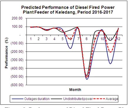
From Table 10 the MAPE calculation for the outages duration is 7.18%. For undistributed power obtained MAPE of -48.27%. Average performance gained -20.54%. Negative MAPE states performance degradation. This mean the diesel fired power plant feeder of Keledang in the Mahakam system is predicted to a 20.54% decrease in performance in 2017. Graphically, the performance is shown

Figure 8. Performance of Diesel Fired Power Plant Feeder of Keledang Period 2016-2017

IV. CONCLUSION

In this study has proven the ability of 1st order FTS to predict the performance of diesel fired power plant feeder through prediction activity of outages duration and undistributed power in actual year and next year. The outages duration and undistributed power prediction results in 2016 resulted in a small MAPE and MSE. This mean the model is good enough used to predict outages duration and undistributed power in 2017. Based on predicted results in 2017, the feeder performance is predicted to decrease by 20.54%. Future work is how to improve feeder performance prediction results by using higher order FTS.

V. ACKNOWLEDGMENTS

The authors would like to express their heartfelt thanks to The Modern Computing Research Center, Department of Information Technology, State Polytechnic of Samarinda for providing all their support.

VI. REFERENCES

1. B. O. lkhine, E. A. Ogujor, and A. E. Airoboman, "Analysis and Development of a Reliability Forecasting Model for Injection Substation," IOSR Journal of Electrical and Electronics Engineering (IOSR-JEEE), vol. 12, pp. 34-38, 2017.

2. T. T and S. K. R, "Smart Grid with Integrating SCADA, GIS and Call Center System for Power Distribution," International Journal of Emerging Research in Management &Technology, vol. 6, pp. 522-527, 2017. 3. F. Postigo Marcos, C. Mateo Domingo, T. Gómez San

Román, B. Palmintier, B.-M. Hodge, V. Krishnan, F. de Cuadra García, and B. Mather, "A Review of Power Distribution Test Feeders in the United States and the Need for Synthetic Representative Networks," Energies, vol. 10, p. 1896, 2017.

4. I. A. Samuel, J. Katende, C. O. A. Awosope, and A. A. Awelewa, "Prediction of Voltage Collapse in Electrical Power System Networks using a New Voltage Stability Index," International Journal of Applied Engineering Research, vol. 12, pp. 190-199, 2017

5. A. M. Al-Shaalan, "Investigating Practical Measures to Reduce Power Outages and Energy Curtailments," Journal of Power and Energy Engineering, vol. 05, pp. 21-36, 2017.

6. T. Cole, D. Wanik, A. Molthan, M. Román, and R. Griffin, "Synergistic Use of Nighttime Satellite Data,

Electric Utility Infrastructure, and Ambient Population to Improve Power Outage Detections in Urban Areas," Remote Sensing, vol. 9, p. 286, 2017.

7. D. H. Didane, N. Rosly, M. F. Zulkafli, and S. S. Shamsudin, "Evaluation of Wind Energy Potential as a Power Generation Source in Chad," International Journal of Rotating Machinery, vol. 2017, pp. 1-10, 2017. 8. I. O. Ogundari, Y. O. akinwale, A. O. Adepoju, M. K.

Atoyebi, and J. B. Akarakiri, "Suburban Housing Development and Off-Grid Electric Power Supply Assessment for North-Central Nigeria," International Journal of Sustainable Energy Planning and Management, vol. 12, pp. 47-64, 2017.

9. P. N. Osakwe, "Unlocking the potential of the power sector for industrialization and poverty alleviation in Nigeria," presented at the United Nations Conference on Trade and Development, 2017.

10. K. A’yun, A. M. Abadi, and F. Y. Saptaningtyas, "Application of Weighted Fuzzy Time Series Model to Forecast Trans Jogja’s Passengers," International Journal of Applied Physics and Mathematics, vol. 5, pp. 76-85, 2015.

11. Z. Abdullah, Z. A. Zakaria, and N. Zamri, "A Comparative Study of Fuzzy Time Series for Rainfall Forecasting," World Applied Sciences Journal, vol. 35, pp. 2119-2123, 2017.

12. N. F. Azahari, M. Othman, and R. Saian, "An enhancement of sliding window algorithm for Rainfall Forecasting," in The 6th International Conference on Computing and Informatics (ICOCI), Kuala Lumpur, 2017, pp. 23-28.