Abstract: Leaf disease detection algorithm using Centroid Distance Neighbourhood Features (CDNF) and Genetic Algorithm (GA) optimization is presented in this paper. This method initially segment the disease affected regions from the leaf. The disease affected region is applied for identifying the best feature points using SURF (Speeded Up Robust Feature) algorithm. From a single SURF point four features are extracted by forming a 5×5 neighbourhood across the SURF feature point. The feature extracted using Centroid Distance Neighbour (CDN) is optimized using genetic algorithm to find best features that are able to classify multiple diseases. During testing phase, the disease region is identified and features points are selected using the SURF points. The features are extracted using the CDN and the necessary features that are optimized by genetic algorithm are sorted out as test features. The test features are classified from the trained features using K-Nearest Neighbour (KNN) algorithm. Performance of the proposed leaf disease detection algorithm is evaluated using metrics such as specificity, sensitivity and accuracy. Experimental results shows that the proposed leaf detection algorithm outperforms the state of-the-art methods and it can be used in real time disease detection.
Keywords: Genetic algorithm, Speeded Up Robust Features, KNN algorithm, Leaf Disease Detection, Centroid Distance Neighbourhood Features (CDNF).
I. INTRODUCTION
The economy of a country highly depends on agricultural productivity. The leaf of a plant or tree usually first expose the diseases present in it. Therefore it is essential to identify the diseases of a tree by diagnosing the disease present in leaf [1]. Early detection of disease in tree or plant avoids the death of tree and increases its life span. Manual identification of leaf diseases is tedious, if the number of plants in a farm is large in number. It also requires experts to identify the plant diseases. Large numbers of experts are required for continuous monitoring of diseases which increases the cost of production. Therefore it is necessary to have an automatic detection system that detects the diseases of the plant by observing the plant leaves. This can be achieved by using computer vision which automatically identifies the disease of plant easily, which makes the diagnosis process easier and cheaper.
To detect plant leaf diseases, the two major processes involved are segmentation [2] and classification [3]. The segmentation process separates the disease affected area of a leaf from the non-affected area.
Revised Manuscript Received on September 03, 2019
Swapna C, Department of Computer Science and Engineering, Noorul Islam Centre for Higher Education, Kumaracoil, Tamilnadu, India.
R.S. Shaji, Department of Computer Science and Engineering, St. Xavier’s Catholic College of Engineering, Chunkankadai, Kanyakumari, India.
The classification process classifies or identifies the type of diseases present in the segmented results. The segmentation algorithm includes edge detection, thresholding, region growing [4], region splitting and merging [5] and snake model such as greedy Snake algorithm [6] and active contour model [7]. Neural networks [8] are also used for the segmentation of the Region of Interest (ROI) from the background. The classification algorithm classifies the different categories of diseases. The classification algorithm includes algorithm such as K-nearest neighbour algorithm (KNN), Fuzzy C-means algorithm (FCM) [9], support vector machines (SVM) [10], convolutional neural networks (CNN) [11] etc.
Hyper-spectral imaging [12] is commonly used in remote sensing where the hyper-spectral sensors capture the image from the near infrared range electromagnetic spectrum. Leaf disease can be detected based on spectral based sensor. In [13], detection of Downy Mildew Disease Fuzzy set theory from Grape Leaves has been proposed. In [14], diseased leaf image classification based on deep neural networks was implemented. This model recognizes 13 different types of diseased plant leaves.
In [15], the gray leaf spot of maize was predicted using recursion and artificial neural networks. It selects the potentially useful predictor variables with the help of correlation and recursion analysis. Nine best predictors are extracted from the leaf and recursion model where used to develop artificial neural networks. They have used 60% of images for training the neural network and 20% of the images for testing and validation. In [16], the wetness of leaf was analyzed and Generalized Recursion Neural Network (GRNN) was proposed to identify plant disease. The leaf wetness was predicted using the micro-meteorological parameters such as wind speed, solar radiation, temperature, precipitation and relative humidity.
The remaining portion of this paper is arranged as follows. Section II explains the proposed leaf disease detection method. Section III displays results and analysis of the proposed work. Finally, conclusion is provided in section IV.
II. METHODOLOGY
This section shows the proposed automatic leaf disease detection algorithm. Fig 1 shows the block diagram of proposed leaf diseases detection algorithm that uses centroid distance neighbourhood algorithm and genetic algorithm optimization. There are two phase involved in this proposed leaf disease classification such
as training phase and testing phase.
Centroid Distance Neighbourhood Features and
Genetic Algorithm Optimization for Leaf
Disease Detection
Fig.1. Block diagram of proposed leaf disease detection method
A. Disease Region Segmentation
The green channel of the leaf image contains more information about the healthy part of the leaf. Let iR, iG, iB be
the Red, Green and Blue channel of the image. The green channel iG is used to detect the diseased region. The disease
region is segmented using thresholding and dilation. The pixels in the green channel iG are iG (x,y). The threshold output
for the image pixels iG (x,y) be IG (x,y) and is given by,
,
1 ,
,
0
G G
if i x y w T I x y
Otherwise
(1)The thresholded image IG (x,y) is a binary image and w is
the weighting factor for threshold T. The threshold T is estimated by using Otsu’s threshold for the image IG (x,y). The
value of w usually lies between 0.5 and 1. The resultant image
IG (x,y) is then dilated using a 3x3 structuring element.
B. Feature Point Identification
In SURF feature extraction, box filters are used, where the scale of box filters is represented as G. For a leaf image u with scale G, the differential operator in x and y direction is represented as DxG and DGy respectively. The size of box filter is l G
[0.8 ]G . The SURF detector is used to detect the feature point in an image. Hessian matrix has good feature detection capability represented as H(x, y, σ).
, ,
,
,
, ,
xx xy yx yy
L x L y
H x y
L x L y
(2)where, σ is the scale and Lxx
x,
is the second order derivative convolution results of Gaussian filter. Let (X,Y) be a SURF feature point. The 5x5 pixel around the SURF feature point at location (X,Y) is used to extract the feature.C. Feature Extraction
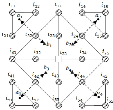
Let (X,Y) represents the position of a SURF featurepoint. The 5×5 neighbourhood of the SURF feature point centered at location (X,Y). From the 5×5 neighbourhood, four features are extracted in diagonal directions. The features are extracted by estimating the distance between the centroid of pixel intensities in diagonal directions as depicted in Fig 2. This proposed feature extraction uses corner centroid and corner facing centroid. The distance between these two centroids is used to extract the feature at a SURF feature point.
Fig. 2. Centroid distance neighbourhood based feature extraction
The four corner centroids are estimated from the corner pixel intensities. Let the four centroids be a1, a2, a3 and a4. For
example, the three top left corner pixels are represented as i11, i12 and i21. The centroid of three top left corner pixel
intensities a1 can be calculated as,
11 12 21 1
3
i
i
i
a
(3) Similarly the centroid for top right corner, bottom left corner and bottom right corner a2, a3 and a4 can be calculatedusing the following equations,
14 15 25 2
3
i
i
i
a
(4)41 51 52 3
3
i
i
i
a
(5)45 54 55 4
3
i
i
i
a
(6) After estimating the corner centroids a1, a2, a3 and a4, thecentroids of intensities facing towards the corner centroids are estimated as b1, b2, b3 and b4.. For example, the Centroid of
intensity b1 facing towards the top left corner intensity a1 can
be calculated using the equation,
13 22 31 32 33 23 1
6
i
i
i
i
i
i
b
(7) Similarly, the centroid of intensities facing towards the top right corner, bottom left corner and bottom right corner a2, a3and a4 can be calculated using the following equations, 13 24 35 34 33 23
2
6
i
i
i
i
i
i
b
(8)31 32 33 43 53 42 3
6
i
i
i
i
i
i
b
(9)33 34 35 44 53 43 4
6
i
i
i
i
i
i
b
(10) The distance between the corner centroid and the centroid facing the corner gives four features, f1, f2, f3 and f4 for the [image:2.595.58.282.68.204.2]1 1 1
f
a
b
(11)2 2 2
f
a
b
(12)3 3 3
f
a
b
(13)4 4 4
f
a
b
(14) D. Feature SelectionThe steps involved in feature selection based on genetic algorithm are initial population, chromosome decoding and design of fitness function. The feature matrix is used to set the initial population. Chromosome decoding provides the permutation of gene and fitness function in an equation that can be used to check the superiority of the given solution. Let
L be the total number of test images and the total features extracted from the a single image is fk,n which is represented as fk,n,l. Where l is the test image number, l=1,2,3……L. The
number of features extracted from one image is given by Eqn.(15).
4
E
N K (15) Let the best feature index b contains B number of elements represented as,
1 2
{ ,
B}
b
b b
b
(16) Therefore the best features are represented by,1 2
1 2
1 2
,1 ,1 ,1
,2 ,2 ,2
,
, , ,
B B
B
b b b
b b b
b l
b L b L b L
F
F
F
F
F
F
F
F
F
F
(17)
The best index b is stored to select the feature from the test image. The feature selection in testing phase is done based on the best index b. During the testing phase, the diseased region is segmented using the segmentation algorithm. The features are extracted from the segmentation image using the proposed feature extraction process.
E. KNN Classification
K-nearest neighbour algorithm stores the features of all training images and classifies the features of test image based on the measurement of similarity. It estimates the distance between the test feature and training features and in the training set that has lowest distance is called nearest neighbour. The distance between the testing feature and a training feature is represented as dist (Fb, Fb,l) ) where Fb is
the set of features selected from the set of features extracted from the test image and Fb,lis the set of features extracted
from the trained image. The distance between the features Fb
and Fb,l can be expressed as,
2,
1
,
,
B
l b b l
b
b b l
d
dis
t
F
F
F
F
(18)1 2 3
{ ,
,
..
}
l L
d
d d d
d
(19)
{ ,
1 2,
3.. }
L
c
argmin d d d
d
(20)The category that belongs to lowest distance features c is retrieved at the KNN output.
III. EXPERIMENTALRESULTS
The performance of the proposed algorithm is evaluated using the plant village dataset [19]. Fig 3 shows some of the leaf disease image samples and healthy image samples from the dataset.
Fig.3. Sample images (a) apple scab, (b) bacterial spot, (c) cercospora leaf spot, (d) common rust, (e) black rot, (d) healthy leaf
We performed classification on leaf diseases such as apple scab, bacterial spot, cercospora leaf spot, common rust, black rot and healthy leaves. In each category, we have classified the complete dataset images into two categories such as training and testing images. The training image consists of 50 images from each categories and testing image consists of 50 images from each categories. The performance was evaluated using metrics such as accuracy, specificity and sensitivity. These metrics can be calculated using the following expressions.
Accuracy(%) tp tn 100
tp tn fp fn
(21)
(%) tn 100
Specificity
tn fp
(22)
(%) tp 100
Sensitivity
tp fn
(23) where,
t
p,t
n,f
pandf
n represents the number of true positive,Fig.4. Results for apple scab affected leaf (a) Original image, (b) Segmented image, (c) Feature point selection using SURF, (d) Pixels used for feature
extraction
[image:4.595.309.544.69.235.2]Various stages of outputs are displayed in Fig. 4. The corner pixels of the SURF points which are used for feature extraction are shown in Fig. 4 (d). Blue color represents the corner pixel on the top left region and green color represents corner pixel on the top right region. Yellow color indicates the bottom left corner and magenta color represents the bottom right corner of the 5×5 neighbourhood. The pixels within this 5x5 region are used to extract the features.
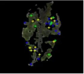
Fig.5. Optimized feature points
Feature points optimized through genetic algorithm are shown in Fig. 5. Blue color indicates that the optimized feature corresponds to top left. Green color indicates that the optimized feature corresponds to top right. Yellow color indicates that the optimized feature corresponds to bottom left. Magenta color indicates the optimized feature corresponds to bottom right.
The genetic algorithm uses population size of 50, number of generations as 100, cross over rate as 0.8 and mutation rate as 0.1. The genetic algorithm converges if the fitness function value is not improved during 100 iterations. The parameters such as sensitivity, specificity and accuracy were evaluated for each category of test images such as apple scab, bacterial spot, cercospora leaf spot, common rust, black rot and healthy leaves. Table 1 shows the percentage of sensitivity, specificity and accuracy for each category of test images.
Table 1 Performance comparison for different categories of leaf diseases with Number of features NE=400
Category Specificity (%)
Sensitivity (%)
Accuracy (%)
Apple Scab 91.99 93.01 96.01
Bacterial Spot 93.76 94.76 96.67
Cercospora Leaf
Spot 92.45 94.88 97.45
Common Rust 93.78 95.12 98.45
Black Rot 94.43 95.34 96.87
Healthy 95.11 95.78 97.67
Overall 93.59 94.82 97.19
Specificity and sensitivity are maximum values for healthy leaf images, while minimum values are obtained for the disease type apple scab. Accuracy is high for the disease type Common Rust and it is low for the disease type apple scab. The overall specificity, sensitivity and accuracy of the proposed classification algorithm are 93.59%, 94.82% and 97.19% respectively. Fig. 6 shows the graphical comparison of sensitivity, Specificity and accuracy for proposed algorithm.
Fig. 6. Performance comparison for different categories of leaf diseases
The performance of the proposed leaf disease detection algorithm is compared with state-of-the-art methods such as Deep Neural Network [14], Hyperspectral Imaging [12], Transfer Learning [17] and Machine Learing [18]. The specificity, Sensitivity and Accuracy of the proposed method was higher than the State of the art methods. The overall Specificity, Sensitivity and accuracy of the proposed method was found to be 93.59%, 94.82% and 97.19% respectively. A performance comparison is provided in Table 2.
Table 2. Performance comparison of proposed method with existing methods
Method Specificity
(%)
Sensitivity (%)
Accuracy (%)
Deep Neural Network
[14] 88.34 89.54 93.42
Hyperspectral Imaging
[12] 89.57 90.03 94.43
Transfer Learning [17] 91.12 92.54 95.56
Machine Learing [18] 91.57 93.12 96.12
[image:4.595.313.543.364.497.2] [image:4.595.99.240.431.555.2]IV. CONCLUSION
A novel automatic leaf disease detection method using Centroid distance neighbourhood features and genetic algorithm optimization is proposed in this paper. Four features are extracted for a single SURF point in diagonal direction. The four features are extracted from the 5×5 neighbourhood of the SURF point. The extracted features are optimized using genetic algorithm. The number of features reduces after optimizing the features. The experimental results were evaluated using the plant village dataset on different types of diseased leaves such apple scab, bacterial spot, cercospora leaf spot, common rust, black rot and healthy images. The overall specificity, sensitivity and accuracy of the proposed leaf disease detection algorithm have been calculated as 93.59%, 94.82% and 97.19% respectively. The experimental results show that the proposed leaf disease detection algorithm outperforms other traditional leaf disease detection algorithms.
REFERENCES
1. Desai, M., Jain, A. K., Jain, N. K., & Jethwa, K. (2016). Detection and classification of fruit disease: A review. Int Res J Eng Technol, 3(3), 727-729.
2. Shijin Kumar P.S and V. S. Dharun." A Study of MRI Segmentation Methods in Automatic Brain Tumor Detection " International Journal of Engineering and Technology 8(2) (2016): pp.609-614.
3. Quirita, V. A. A., da Costa, G. A. O. P., Happ, P. N., Feitosa, R. Q., da Silva Ferreira, R., Oliveira, D. A. B., & Plaza, A. (2016). A new cloud computing architecture for the classification of remote sensing data. IEEE Journal of Selected Topics in Applied Earth Observations and Remote Sensing, 10(2), 409-416.
4. Zhang, Y. J., 1997. Evaluation and comparison of Different segmentation algorithms. Pattern Recognition Letters, 18(10). Pp. 963-974.
5. S.K Somasundaram, P.Alli,” A Review on Recent Research and Implementation Methodologies on Medical Image Segmentation”, Journal of Computer Science 8(1): 170-174, 2012.
6. C. Jaspin Jeba Sheela, G. Suganthi. (2019). Automatic Brain Tumor Segmentation from MRI using Greedy Snake Model and Fuzzy C-means Optimization, Journal of King Saud University -Computer and Information Sciences.
7. E. Ilunga-Mbuyamba, J.G. Avina-Cervantes, A. Garcia-Perez, R. de J. Romero-Troncoso, H. Aguirre-Ramos, I. Cruz-Aceves, C. Chalopin, Localized active contour model with background intensity compensation applied on automatic MR brain tumor segmentation, Neurocomputing. 220 (2017) 84-97.
8. Shijin Kumar P.S and Sudhan M.B. "A Hybrid Framework for Brain Tumor Detection and Classification using Neural Network" ARPN Journal of Engineering and Applied Sciences 13(24) (2018): pp.9631-9636.
9. Shijin Kumar P.S and V. S. Dharun. "Combination of Fuzzy C-means Clustering and Texture Pattern Matrix for Brain MRI Segmentation." Biomedical Research 28(5) (2017): pp.2046-2049.
10. Hari Babu Nandpuru, Dr. S. S. Salankar, Prof. V. R. Bora, “MRI Brain Cancer Classification Using Support Vector Machine, IEEE Students' Conference on Electrical, Electronics and Computer Science, 2014. 11. Chen Y, Jiang H, Li C, Jia X, Member S. Deep feature extraction and
classification of hyperspectral images based on convolutional neural networks. IEEE Trans Geosci Remote Sens 2016; 54(10):6232–51. 12. Lowe A, Harrison N, French AP. Hyperspectral image analysis
techniques for the detection and classification of the early onset of plant disease and stress. Plant Methods 2017;13(1):80.
13. Kole DK, Ghosh A, Mitra S. Detection of downy mildew disease present in the grape leaves based on fuzzy set theory. Advanced computing, networking and informatics. Switzerland: Springer; 2014. p. 377–84. 14. Sladojevic S, Arsenovic M, Anderla A, Culibrk D, Stefanovic D. Deep
neural networks based recognition of plant diseases by leaf image classification. Comput Intell Neurosci 2016;2016:1–11.
15. Paul PA, Munkvold GP. Regression and artificial neural network modeling for the prediction of gray leaf spot of maize. Phytopathology 2005;95(4):388–96.
16. Chtioui Y, Panigrahi S, Francl L. A generalized regression neural network and its application for leaf wetness prediction to forecast plant disease. Chemom Intell Lab Syst. 1999;48(1):47–58.
17. Hasan, Mosin and Tanawala, Bhavesh and Patel, Krina J., Deep Learning Precision Farming: Tomato Leaf Disease Detection by Transfer Learning (March 9, 2019). Proceedings of 2nd International Conference on Advanced Computing and Software Engineering (ICACSE) 2019.
18. Puspha Annabel, L. S., Annapoorani, T., & Deepalakshmi, P. (2019). Machine Learning for Plant Leaf Disease Detection and Classification – A Review. 2019 International Conference on Communication and Signal Processing (ICCSP).
19. https://github.com/spMohanty/PlantVillage-Dataset/tree/master/data_d istribution_for_SVM.
AUTHORSPROFILE
C. Swapna obtained her MCA degree from Annamalai University, Chidambaram. She is pursuing her PhD in Computer Science and Engineering at Noorul Islam Centre for Higher Education, Kumaracoil, Tamilnadu. Her area of research interest includes, pattern recognition, machine learning and image processing. She is currently working as Assistant Professor in the University Institute of Technology, University of Kerala. She is having 26 years of experience in teaching and 3 years experience in software industry.