A model for assessing iceberg hazard

White Rose Research Online URL for this paper:

http://eprints.whiterose.ac.uk/129330/

Version: Published Version

Article:

Bigg, G.R. orcid.org/0000-0002-1910-0349, Cropper, T.E., O’Neill, C.K. et al. (7 more

authors) (2018) A model for assessing iceberg hazard. Natural Hazards. ISSN 0921-030X

https://doi.org/10.1007/s11069-018-3242-x

[email protected] https://eprints.whiterose.ac.uk/

Reuse

This article is distributed under the terms of the Creative Commons Attribution (CC BY) licence. This licence allows you to distribute, remix, tweak, and build upon the work, even commercially, as long as you credit the authors for the original work. More information and the full terms of the licence here:

https://creativecommons.org/licenses/

Takedown

If you consider content in White Rose Research Online to be in breach of UK law, please notify us by

O R I G I N A L P A P E R

A model for assessing iceberg hazard

Grant R. Bigg1 •T. E. Cropper1•Clare K. O’Neill2•Alex K. Arnold2• A. H. Fleming3•R. Marsh4•V. Ivchenko4•Nicolas Fournier2• Mike Osborne5•Robin Stephens6

Received: 17 June 2016 / Accepted: 22 February 2018

Ó_{The Author(s) 2018. This article is an open access publication}

Abstract With the polar regions opening up to more marine activities but iceberg numbers more likely to increase than decline as a result of global warming, the risk from icebergs to shipping and offshore facilities is increasing. The NW Atlantic iceberg hazard has been well monitored by the International Ice Patrol for a century, but many other polar regions have little detailed climatological knowledge of the iceberg risk. Here, we develop a modelling approach to assessing iceberg hazard. This uses the region of the Falklands Plateau and its shipping routes for a case study, but the approach has general geographical applicability and can be used for assessing iceberg hazard for routes or fixed locations. The iceberg risk for a number of locations selected from the main shipping routes in the SW Atlantic is assessed by using an iceberg model, forced by the output from a high-resolution ocean model. The iceberg model was seeded with icebergs around the edge of the modelled region using a number of scenarios for the seeding distribution, based on a combination of idealised, modelled and observed iceberg fluxes from the Southern Ocean. This enabled us to determine measures of iceberg risk linked to a mix of starting location and the likelihood of icebergs being encountered in such a position. For our study area, the main area of iceberg risk is linked to the East Falklands Current, but small, yet nonzero, risk covers much of the east and north of the region.

Electronic supplementary material The online version of this article (https://doi.org/10.1007/s11069-018-3243-x) contains supplementary material, which is available to authorized users.

& _{Grant R. Bigg}

[email protected]

1 _{Department of Geography, University of Sheffield, Winter Street, Sheffield S10 2TN, UK}

2

Met Office, Fitzroy Road, Exeter, Devon, UK

3 _{British Antarctic Survey, High Cross, Madingley Road, Cambridge, UK}

4

National Oceanography Centre, University of Southampton, European Way, Southampton, UK

5 _{Premier Oil plc, 23 Lower Belgrave Street, London, UK}

6

Keywords IcebergModellingRisk assessmentFalklandsIceberg

hazard

1 Introduction

Icebergs have been a hazard to shipping for centuries, ever since the first voyages of Euro-peans to Greenland, NE America and Svalbard. From the first recorded sinking due to an iceberg, of the North West Fur Company’sHappy Returnin the Hudson Strait in 1686 (Hill

2000), sailing into the Labrador Sea, in spring and early summer in particular, has been hazardous. As maritime trade increased through the nineteenth and early twentieth centuries, collisions with icebergs steadily increased, with 26% of such incidents leading to sinkings or abandoned vessels (Hill2015). The tragic disaster of the sinking of RMSTitanicon 14 April 1912, with the loss of over 1500 lives, was a catalyst for the creation of the International Ice Patrol (IIP). This has now accumulated a century of observational and ice hazard warning experience in the NW Atlantic (Murphy and Cass2012), reducing the number of iceberg collisions drastically to an average of between 0 and 2 a year (Hill2015), despite the level of global shipping now being 8 times that in 1912 (Bigg2016). Such long-term monitoring has resulted in an experienced observational and prediction service (Koonar et al.2004).

However, other parts of the globe have an iceberg hazard (Berz et al.2001), but do not have such a good observational base concerning past iceberg numbers and distributions, nor a long-established ice hazard service. A few regions have collections of ship or drift buoys’ observations of icebergs, such as the Barents Sea (Abramov1992; Eik2009), West Greenland (Valeur et al.1996; Fournier et al.2013; Larsen et al.2015), the Grand Banks (Verbit et al.

2006) or parts of the Southern Ocean (Jacka and Giles2007; Romanov et al.2008). Others have satellite-derived records. The Southern Ocean has a scatterometer-derived series of giant icebergs (length,Li[10 nautical miles or 18.5 km), continuous since 1992 (Stuart and

Long2011), and an altimeter-derived distribution of small-sized icebergs (Li, 100–2800 m)

north of 70°_{S since 1992 (Tournadre et al.2016). However, neither the ship-based}

obser-vations nor the satellite data provide long timeseries of the full iceberg distribution over the Southern Ocean or the Arctic. Therefore, in most parts of the polar regions subject to an iceberg hazard there is insufficient past information for there to be a good understanding from climatology of the risk of iceberg presence. Those companies working in polar or sub-polar waters subject to potential iceberg collision risk beyond the NW Atlantic are increasingly using external services to monitor, and if necessary, track icebergs entering danger zones for their operations. Synthetic aperture radar (SAR) satellite information provides the ability to resolve individual icebergs down to a few tens of metres in size from recently flown sensors. Nevertheless, monitoring current iceberg movement in limited regions does not provide a measure of the long-term iceberg risk, particularly during a changing climate.

A climatological view of ocean basin-scale to global iceberg distributions has been provided from past iceberg modelling simulations. A North Atlantic and Arctic modelling perspective of iceberg distribution was provided in the mid-1990s (Bigg et al.1996), with horizontal resolution down to 0.25° _{in the NW Atlantic (Bigg et al. 1997). A similar}

sheets, to produce distributions from sets of trajectories; all of the above used climato-logical forcing. Only one global simulation has attempted to use a long-term atmospheric reanalysis—the imperfect Twentieth Century Reanalysis—as forcing to produce a century-long temporally varying iceberg distributions (Bigg et al.2014; Wilton et al.2015). This simulation reproduces the annual IIP timeseries of iceberg numbers crossing 48°_{N in the}

Labrador Sea reasonably well and has the same decadal-scale variability as ice-rafted debris in marine cores in the Denmark Strait (Andrews et al.2014). However, this veri-fication is only for these two distinct locations and cannot be guaranteed to extend well beyond the NW Atlantic, or into near-shore and high-polar regions where tidal oscillations and inertial oscillations have a strong impact on iceberg drift patterns.

Thus, a method to determine the iceberg risk for a region outside the NW Atlantic is still awaited. In this paper, we provide a methodology to tackle this problem, using a range of iceberg distribution scenarios along the perimeter of a study area. For the latter we chose the Falklands Plateau, because of the combination of a known, if low, iceberg risk in the area, a significant, and varied range of exposed shipping routes, the likely future deployment of offshore marine platforms, and the availability of a very-high-resolution 20-year ocean simulation which can be used to force our set of iceberg scenarios. However, the general approach presented here is generic and could be applied anywhere.

2 Data and methods

2.1 Region of study

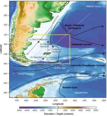
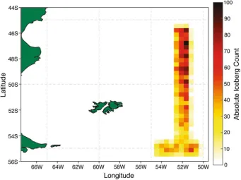
Historically, the SW Atlantic (Fig.1) was a region of major maritime trade routes, with vessels travelling from Europe and NE America to the west coast of the Americas or the Pacific Islands having to pass through the Strait of Magellan, or around Cape Horn, before the Panama Canal opened in 1914. During the latter half of the nineteenth century, there were frequent references to significant regions of ice and icebergs in the Southern Ocean north of latitudes where they are commonly encountered today (Brett1924). During the 1890s, ice was frequently encountered off Cape Horn and into the seas up to a week’s sailing north of the Falkland Islands (Lubbock2008). These sightings included icebergs described as 20 miles and 40–50 miles in length, respectively. Admiral Von Spee’s battle squadron encountered a ‘‘huge iceberg’’ just off Cape Horn in December 1914, on their way to the Battle of the Falklands (Hough2003). Occasional giant icebergs calved from the Amundsen Sea will track through the Drake Passage, as iceberg B10a did in late 1999. These can potentially enter the East Falklands Current. There remain occasional sightings of icebergs in Falkland Islands waters, and even a past grounding on Burdwood Bank, 150 km south of the islands. It is also noteworthy that there are extensive records of iceberg scour in sediments dating from the last glacial period west and north of the Falklands (Brown et al.2017).

mean location represents the low traffic routes south-east towards the Antarctic and South Georgia. These specific locations are given in Table1.

2.2 Ocean model

The ocean model used in this study is a regional Nucleus for European Modelling of the Ocean (NEMO; Madec (2008)) configuration that was set up by the Met Office to cover the Patagonian Shelf region, here referred to as the PS4 model. The PS4 model grid covers the region 70°_W–50°_{W, 56}°_S–44°_{S using a regular grid with horizontal resolution 1/12}°_in

longitude and 1/16°_{in latitude. This is equivalent to approximately 7 km at the considered}

latitudes and allows fine mesoscale features to develop.

The main set-up and parameterisations are based on the Met Office AMM7 configu-ration (O’Dea et al. 2012). This is a well-established model of the Northeast Atlantic region which has the same resolution and covers a similar latitude range as PS4 (albeit in the Northern Hemisphere). AMM7 is run operationally at the Met Office for forecasting in European Waters and is also used to provide multi-year reanalyses.

In the vertical, the PS4 model has 51 depth levels using the terrain-following hybrid coordinate system of Siddorn and Furner (2013). In this scheme, the model levels are evenly spaced throughout the water column in shelf regions, avoiding excessively thin layers, whereas in deeper regions they are spaced to retain increased resolution at the surface. In areas of very steep topography, the use of terrain-following coordinates can lead to errors in calculation of the horizontal pressure gradient (Mellor et al. 1994). This is reduced in PS4 by using a smoothed ‘‘envelope’’ bathymetry for the calculation of the model levels, reducing the steepness of the levels without distorting the shape of the bathymetry that is used by the model. The Siddorn and Furner scheme also allows the surface layer thickness to be kept constant across the domain, improving the treatment of air-sea fluxes. For the PS4 configuration, we specify a surface layer of 1 m.

The time-stepping scheme used is a time-splitting formulation where the free surface and barotropic velocity equations are solved with a shorter timestep than that used for baroclinic variables. The PS4 configuration uses a baroclinic timestep of 180 s with a barotropic sub-timestep of 6 s.

Lateral boundary forcing for the PS4 model was taken from the Met Office GloSea5 system (MacLachlan et al. 2014), a global coupled ocean–atmosphere seasonal forecast system. GloSea5 uses the°_{ORCA025 NEMO model as its ocean component, which is}

well established and validated (for example, Blockley et al.2014).

The variables that are specified at the open boundaries are daily temperature, salinity, sea surface height and barotropic velocity. Temperature and salinity are applied using a flow relaxation method (Martinsen and Engedahl1987), in which the boundary zone is specified as a region 10 grid points wide. The model variables in the boundary zone are relaxed to those Table 1 Location of points on

shipping routes where iceberg fluxes are considered in more detail

Shipping route Study point

Strait of Magellan (1) 47°_{S, 63}°_W Falkland Islands N (2) 47°_{S, 59}°_W Falkland Islands NE (3) 49°_{S, 57}°_W

Cape Horn (4) 54°_{S, 61}°_W

from the external model (i.e. GloSea5) such that values on the outer edge of the domain are entirely prescribed by the external model and its influence rapidly decreases as we move further inwards across the boundary zone. Barotropic variables are applied using the Flather (1976) radiation condition. This is a scheme in which the depth mean velocity normal to the boundary is set equal to that in the external model, but with an adjustment that allows gravity waves generated within the nested model to exit through the boundaries.

In addition, tidal forcing was included in the PS4 model by specifying tidal harmonics at the boundaries for eight harmonic constituents: K1, K2, M2, N2, O1, P1, Q1, S2 (Pugh and Woodworth 2014). The tidal forcing data are provided by the BMT ARGOSS in-house tidal model. The model has a spatial resolution of 0.1°_{and is based on the integration of}

approximately 5000 tidal stations and 13 years of satellite radar altimeter observations into depth average global and regional tidal models (2DH model).

Surface heat and salt fluxes were calculated using the CORE bulk formulation (Large and Yeager2004). Use of a bulk formulation allows model sea surface temperature (SST) feedback into the calculation of the fluxes and results in more physically accurate surface boundary conditions than possible when using direct flux forcing. The CFSR reanalysis data set (Saha et al.2010) was used to provide the required atmospheric parameters: wind, sea-level pressure, relative humidity, air temperature, precipitation and snowfall. This data set provides hourly data with a spatial resolution of 0.5°. An example of annual mean wind field across the PS4 model region is shown in Fig.2.

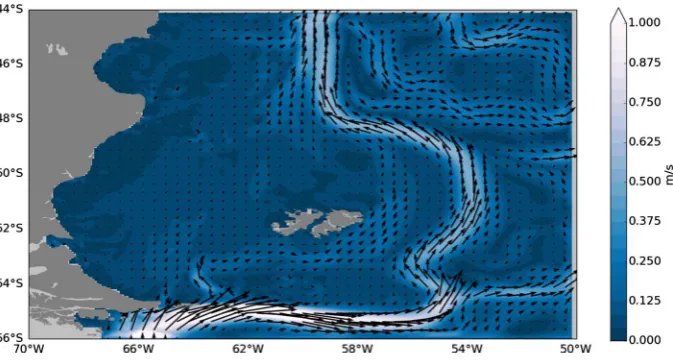
The PS4 model was run for a 20-year period, from 1993 to 2012. The initial density field was taken from GloSea5, and the model allowed to spin up for 2 years before beginning the main run. Hourly snapshot values were output for the whole 20-year period. Example of annual mean SST and surface current fields is shown in Figs.3and4, respectively.

2.3 Iceberg model

The iceberg trajectory model used here derives from that developed by Bigg et al. (1997) and modified by Gladstone et al. (2001) and Levine and Bigg (2008). It includes both

Fig. 2 Contour diagram of the annual mean wind strength for 2012, with the 5.2 ms-1

dynamical forces to move the icebergs and thermodynamics to provide melting during transit. Full details of the model formulation are provided in these references; however, the dynamical forces affecting the individual icebergs are ocean, atmospheric and (if present) sea-ice drags, the Coriolis force, pressure gradients in the surrounding ocean and a wave radiation force. The dominant force tends to be the water drag, but, particularly in strong winds, other terms such as the wave radiation stress and air drag may become as important at times (Bigg et al.1997). In our simulations, sea-ice is not present at any time due to the sea surface temperature always remaining above freezing point, so this force component is never applied. Note that icebergs may roll over if the Weeks–Mellor stability criterion (Weeks and Mellor1978) is not met.

Fig. 3 Contour diagram of the annual mean model sea surface temperature for 2012

The thermodynamical processes contributing towards changing the mass of each ice-berg are basal melting, buoyant convection, wave erosion, sublimation, latent heat transfer and the addition of mass through snowfall. In addition, if icebergs enter water shallower than their draught, then they ground and melt until their draught is reduced to below the local water depth. For simplicity of calculation, all icebergs simulated are rectangular in shape, with a width/length ratio of 1:1.5, this being similar to mean ratios found in both hemispheres. A ratio of draught to freeboard of 5:1 is assumed; again, this is more con-sistent with observations of the most common real icebergs of tabular and wedge shapes (Fequet 2002) than just assuming the buoyancy to be directly linked to the density dif-ference between ice and seawater (see Bigg et al. (1997) for a full discussion of these ratios). Again, for simplicity of calculation all icebergs are assumed to be travelling with their long axes parallel to the surrounding water flow, but with the atmospheric wind direction being 45°_{to the right of the iceberg. This is consistent with Ekman theory in the}

mean, but will not always be the case in reality. As icebergs melt, their loss of mass is redistributed after calculation at each time step so as to maintain the ratios given above over time. Once modelled icebergs approach growler size (*5 m), they are assumed to

instantaneously melt, for numerical stability.

Previous studies have used a range of time steps for the iceberg model, from order 1–200 s (Bigg et al.1997) to order 10,000 s (Levine and Bigg2008), depending on the timescales the respective models were considering. Here, to best estimate the iceberg hazard for a particular location, we wish to retain as much of the iceberg dispersion from short-term current variation as possible, while also minimising computational costs. The ocean model data used as forcing for the iceberg model were available as hourly snapshots, so 3600 s is the maximum time step we considered suitable. However, we tried a range of time steps (100, 200, 400, 600, 3600 s) to see whether more dispersive, and more realistic, iceberg distributions required shorter time steps. The resulting dependence of iceberg distribution on time step from a full 20-year run using seeding from scenario 2 (see the next section) is shown in Online Resource 1. This suggests that a maximum time step of 200 s both retains reasonable dispersion, while minimising computational cost. This is very similar to the 180-s time step of the ocean model. However, the simulations used here employ the 100-s time step (shown in Fig.5), so as to maximise the dispersion characteristics.

2.4 Experiment scenarios

We considered three scenarios for iceberg seeding of our model region, to give us measures of the ‘‘possible’’ iceberg hazard ranging to the ‘‘probable’’ hazard. Scenario 1, hereafter SC1, addresses the possible hazard question, giving us a maximal baseline against which to compare the more realistic scenarios. Icebergs of a uniform 200 m length and depth were released every 30 days at evenly spaced intervals of four ocean model grid points (*0.4°)

near both the southern and eastern boundaries of the ocean model domain. The width of the icebergs followed the width/length ratio of 1.5 noted earlier. The uniform release locations are shown in Fig.1; a total of 88 icebergs are released on each occasion. For numerical stability and to avoid the ocean model relaxation zone, the icebergs were released 10 ocean grid points in from the boundary (1°) and were initially at rest. By releasing icebergs frequently along the southern and eastern edges of the study area, SC1 gives a maximal measure of the possibility of an iceberg reaching a particular location.

Note, however, that this is not the actual probability of occurrence at a location, as the likelihood of an iceberg crossing the boundary of the study area is far from spatially uniform. This is known from the limited satellite observations (Tournadre et al.2016) and also from model simulations (Marsh et al.2015; Wilton et al.2015), both of which show that the likelihood of an iceberg entering along the southern boundary west of*55°W is

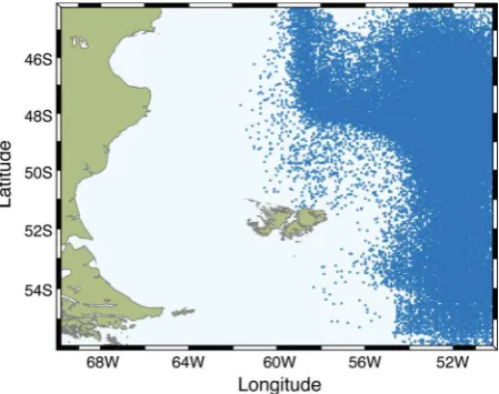
very small. Scenario 2, hereafter SC2, was created in order to provide a more realistic estimate of the probability of experiencing iceberg hazard. This scenario was guided by the iceberg distribution found from icebergs simulated during years 10–14 of the 0.25°

reso-lution simulation (ORCA025) of the coupled ocean-iceberg model NEMO-ICB discussed in Marsh et al. (2014). While a longer simulation of this model has since been run (Marsh et al.2015), the general results of the original simulation are compatible with this longer simulation and also with the iceberg distributions from the *1° resolution Twentieth

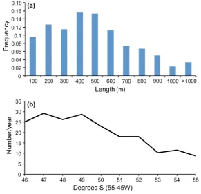
Century coupled ocean-iceberg simulation of Wilton et al. (2015). The icebergs calved from the coast of Antarctica in ORCA025 ranged in size from 50 to 1500 m in length, and up to 300 m in depth, and the simulations resulted in*240 icebergs reaching the eastern

edge of the study area each year, with horizontal sizes varying over 100–1100 m (Fig.6). These occurred most frequently in the northern half of eastern boundary. Only one of these icebergs reached the southern edge of the region during the simulation. SC2 takes this record into account by allowing 20 icebergs to enter the eastern part of the study area each month (i.e. 240 a year), with a random component altering the actual location and size of the icebergs seeded in any given month, although with a maximum depth of 300 m, while the overall distribution of seeded iceberg size was determined by the distributions shown in Fig.6. The resulting seed density over a typical 20-year simulation is shown in Fig.7, giving the equivalent of 240 icebergs crossing through the release zone each year, as was found in Marsh et al. (2014). In addition, a number of variants of SC2 were run, where the order of seeding of the 20-year set of iceberg seeds was shifted, so as to allow different ocean and atmospheric forcings to perturb the basic regional iceberg distribution.

variation in upper ocean forcing of the icebergs’ behaviour, and so is a supplement to SC2 rather than a radically different estimate.

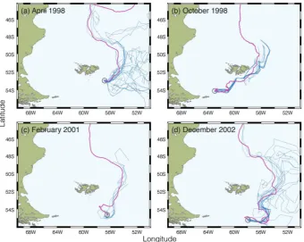
2.5 Model verification using surface drifters

we simulated the paths of drifters that entered our region, representing them as icebergs, through a range of months of the year over the decade of 1997–2006. The pseudo-icebergs were given the initial position and velocity of the drifter, but with a number of icebergs being released at the same time from slightly different start positions (between 0.06°_and

0.25°_{from the drifter location), so as to examine the sensitivity of the iceberg model to}

initial position. Drifters are, of course, not icebergs, with a much lower mass, depth and size, meaning that there are likely to be significant differences in the force balance between a drifter and iceberg released in the same location. The ocean model circulation will also not faithfully reproduce the small-scale flow turbulence that the drifter, in particular, will experience. Therefore, the paths of model icebergs of the standard 200 m size, which melt over time, will not exactly follow the drifter tracks. However, Fig.8shows that the drifter tracks typically lie within the envelope of the modelled iceberg swarm. This gives con-fidence in the iceberg hazard estimates given below. The degree of divergence in these examples is strongly linked to the wind field for the month. Both in April 1998 and in December 2002 (Fig.8a, d), the drifters moved through strong changes in wind speed, leading to more separation of the drifter and model icebergs. In contrast, in October 1998 and February 2001 (Fig.8b, c) the drifters remained in areas of similar, or rapidly decreasing wind field. Variation in the wind effects on iceberg motion would have therefore been less in these months.

3 Scenario results

3.1 Mean forcing on iceberg motion

The major two controls on iceberg movement are the ocean currents and near-surface winds. Typically, wind speeds of less than about 5.2 ms-1_{have little control on iceberg}

direction but sustained (at least 6 h) 10-min mean wind speeds[5.2 ms-1have a greater effect (Ettle1974; Turnbull and Fournier2015). There is a transition between mean wind speeds greater than this value to the south of a line extending roughly from the Strait of Magellan north of the Falklands to the NE corner of the domain (Fig.2), weaker winds being to the north-west. The major ocean current throughout the region is the Falkland Current (Fig.4). This current originates in the south-west corner of the domain below Staten Island and flows in an easterly direction along*55°S until it reaches*55°W.

There the flow changes direction and flows on a northerly route until*49°–50°S where it

then changes direction again and flows in a westerly direction until*48°S, 59°W where it

then flows northwards, out of the domain. There is another, weaker, current that takes a similar path, but much closer to the Falkland Islands. This bifurcates from the major Falkland Current flow around 55°_{S, 63}°_{W. This current will be referred to as the Inner}

65°_{W (the daily tidal regime) and in the north-eastern corner (east of 55}°_{W, equatorward}

of 48°_{S), where the Brazil–Falkland Confluence occurs.}

Throughout the year, the SST across the whole region is above *3°C, allowing

significant melting of icebergs to occur (Fig.3). The SST approaches 15°_{C widely across}

the northern half of the domain during summer and autumn, ensuring few seeded icebergs reach the northern edge of the study area. However, the Falkland Current transports sig-nificantly colder surface water from the Southern Ocean in a narrow band northwards, along which many of the icebergs observed in the past will have travelled (e.g. Lubbock

2008), minimising the melting along the major iceberg zone.

In the remainder of the results section, we consider the trajectories and densities of icebergs seeded into the model using the scenarios discussed in Sect.2.4.

3.2 Scenario 1

An iceberg density map for SC1 is shown in Fig.9, derived from the full set of monthly releases over 1993–2012. The darker colours, indicating a higher iceberg density, are spread linearly around the edge corresponding to the iceberg seed positions, as would be expected. A high iceberg density is also shown for the Falkland Current, which is the feature dominating the iceberg density count. Note that modelled icebergs are grounded off the Falkland Islands and the Argentine coast around 48°_{S. In the grounded cases, a high}

density exists as the icebergs may remain in the same position for weeks to months before melting, meaning that the same iceberg is repeatedly counted. It should be remembered

that SC1 is a baseline study, showing where icebergs could possibly travel within the study area from an unrealistic, but maximal, release strategy.

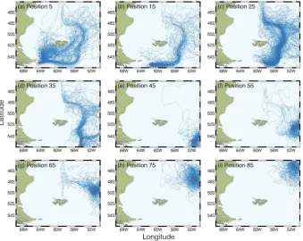
Iceberg tracks from various release positions from SC1 are shown in Fig.10. The majority of icebergs from the southern seed positions end up within the main Falkland Current. Modelled icebergs from release positions along the southern boundary from Cape Horn to*63°W can, on occasion, be entrained within the Inner Falkland Current that

passes much closer to the Islands, or can even be found west of the Falkland Islands. Modelled icebergs along the eastern boundary are occasionally entrained within the main Falkland Current; this is particularly likely from releases around both 54° _{and 49}°_S.

Variability on the sub-monthly temporal scale, which can come from short-term wind and current changes, will be the major cause of icebergs escaping the major currents and crossing onto the Shelf.

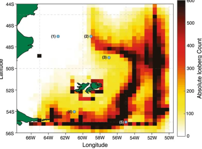
To determine the risk of an iceberg from any possible entry point into our domain reaching a given internal location, we examine the number, and properties, of icebergs from SC1 that reach the five locations on the main shipping routes, as given in Table1. The total number of unique icebergs reaching these locations from all entry points is listed in Table2. Remembering that SC1 is about what is possible, rather than what is probable, there are distinct differences between the threat of icebergs reaching these five locations. Only 11 of the 21,120 icebergs released during this experiment pass within 1°of location 1, and none within 10 km. Both the Falkland Island shipping route locations, and that for the Cape Horn route (2–4), had 6–8% of the released icebergs reaching within 1°_{of the sites,}

with just a few dozen approaching within 10 km. In contrast, the Antarctic route example (5) had 25% of the released icebergs pass within 1°_{. This route crosses the Falkland}

Current; many model icebergs are entrained into this current, leading to the high numbers. The closeness of the locations to the release points leads to dramatically different changes in size of the icebergs en route (Fig.11). Those few reaching location 1 have travelled a long way, having had both their length and depth more than halved, with over 50% reduced to a quarter or less of their original dimensions. This is more so for the depth, on which the major, basal, melting term acts. The Falkland route locations (2, 3) have shorter travel paths, but in warmer waters. Thus, their modal response is to lose half their depth from melting, but all lengths possible are found, depending on the details of indi-vidual trajectories. Both the Cape Horn and Antarctic routes (4, 5) are close to the release lines, so the modelled icebergs reaching these locations have only small decreases in both their mean depth (Fig.11b) and length (Fig.11a). Only very few, having taken unusual paths to reach these locations, lose 50% or more of their mass.

3.3 Scenario 2

SC2 iceberg seed positions and number density are given in Fig.7. A set of nine ensembles of SC2 were run, with positions and sizes of seeded icebergs varying randomly but in overall accordance with the distributions in Fig.6. The SC2 ensemble average iceberg density and standard deviation are both shown in Fig.12. The ensemble mean shows the highest density around the seed positions and immediately to the east, where the majority of seeded icebergs rapidly leave the domain. Within the main domain, the principal density peak follows the northern branch of the Falkland Current, but with some dispersion around 48°_{S, 58}°_{W, where the current is guided by the continental slope in a sharp transition from}

a zonal to meridional configuration. Eddies tend to be shed from the current in this region, as suggested by the bifurcation of the mean model ocean current shown in Fig.4, the simulations of Hallberg and Gnanadesikan (2006) and satellite altimetry observations (Ducet et al.2000). This tendency for mesoscale variability lies behind the high ensemble standard deviation on the shelf side of the Falkland Current in this general region (Fig.12b). This arises because of high iceberg counts in one or two ensemble runs, and Table 2 Number of unique model icebergs from different scenarios found in the vicinity of the five shipping route locations of Table1over 20-year simulations

Location SC1 SC2 SC3

B1° radius

B50 km B10 km B1° radius

B50 km B10 km B1° radius

B50 km B10 km

1 11 6 0 0 0 0 0 0 0

2 1245 960 62 242 212 11 337 271 21

3 1720 525 39 253 34 2 332 47 5

4 1430 396 37 0 0 0 0 0 0

5 5334 3261 65 161 60 0 175 63 1

low/zero counts in others, depending on the precise release positions and sizes of seeded icebergs in different runs making up the ensemble.

Each of the other locations has *150 to 250 icebergs approach within 1° over the

20 years of the simulation, with site 2 (Falkland Islands—North) being more likely to have icebergs approach more closely. This is because site 2 is very near the sharp veering of the Falkland Current from westwards to northwards near 48°_{N, 60}°_{W (Fig.1), this current}

carrying the majority of the icebergs that enter the Falklands area (Fig.5). Nevertheless, the risk, while finite, is low. An average of*10 icebergs approaches this site per year in

the simulation, but only one every other year approaches within 10 km.

Only three of the locations of Table2have icebergs approach them in SC2, so Fig.13, showing the distribution of the SC2 icebergs’ length and depth, has only three bars per category. All three of the locations 2, 3 and 5 are relatively close to the release zone for SC2 (Fig.7). Thus, the depth of 50% of the icebergs changes by less than 10%, with smaller proportions of icebergs reducing by greater amounts. Those losing more mass will have travelled further since release in the Falkland Current, further south. There is a similar relatively small loss in length in each region, remembering that initial icebergs in SC2 varied randomly in length between 100 and 1100 m, but driven by the distribution shown in Fig.6a. There is greater erosion in both length and depth for those icebergs reaching

location 5, in the Antarctic route. Icebergs here will have been entrained into the Falkland Current near the south-east corner of the domain and thus travelled further than those released on the eastern side further north and travelling to locations 2 and 3.

3.4 Other scenarios

Experiment SC3 is a sensitivity study of SC2, where the iceberg seeding is identical, but the icebergs’ dynamics and thermodynamics were driven by sub-surface velocities and temperatures. However, this has relatively little impact on the mean characteristics of the trajectories compared to those of SC2. This is particularly true of the mean dimensions of the icebergs reaching the general area of each of the three locations (2, 3 and 5); these are shown in Fig.14and are very similar to those for SC2 in Fig.13. However, more icebergs do reach the three locations, as shown in Table2, mostly because the melting is reduced by the lower mean ocean temperature affecting the submarine faces of the icebergs. The risk of a location having an iceberg pass within 10 km thus roughly doubles, to around one iceberg per year on average.

Other scenarios were examined, for example, varying the flux through the year by having the majority of the icebergs seeded in either the winter or summer. However, the impact of these scenarios on the results of SC2 was minimal in terms of the numbers and dimensions of icebergs encountered near the selected locations and will not be considered further.

4 Measuring and monitoring risk

The results of SC1-3 can be used to estimate an encounter rate of each fixed location given in Table1. As we have seen, there are a range of possible dimensions of icebergs that may reach each location. Only the length is of interest here. To calculate an encounter rate, it is assumed that all icebergs modelled to approach within 10 km of the location are of a maximum likely horizontal size (10009667 m, to follow the 1.5:1 size ratio (Bigg et al.

1997)). A more typical encounter rate, reflecting the dimensions of the SC1 releases, and the smaller quarter of the icebergs reaching the locations in SC2 (Fig.13), of 2009133 m are also calculated. The encounter rate is calculated by dividing the area of the icebergs entering a 10-km-radius circle around the location on average each year of the simulation by the area of the 10-km circle. The results of these calculations are given in Table3.

The largest likely encounter rate (from SC2 or SC3) for the more typical length icebergs (200 m) is at site 2, being*1 in 11,000 years. This is reduced by a factor of 4 for site 3,

and 20 for site 5, to much less than 1 in 100,000 years. If all icebergs reaching the fixed locations were of a maximum size (1000 m), then the encounter rate is much higher, with the greatest being 1 in 330 years at site 2. Of course, the realistic encounter rate is somewhere in between these extremes and, given that *5% of icebergs reaching our

locations (Figs.13and14) are of the maximum size; then, this will be*1 in 4200 years

at site 2 and much less at sites 3 and 5.

The encounter rates calculated from the implausible baseline SC1 are significantly higher, and taking into account that the maximum length of a released iceberg here was 200 m then the rate is *1 in 3500 years, and 1 in 130 years if 1000 m in length.

However, icebergs are not, in reality, released from all places along the eastern and southern boundary each month, so the encounter rate calculations from SC2 or SC3 are more realistic.

As well as an estimate of an encounter rate, this approach to investigating iceberg risk provides a basis for its monitoring. The likely origin of icebergs that may affect given shipping routes or fixed locations can be determined by the trajectory modelling, including

Table 3 Encounter rate for icebergs at the five locations given in Table1, using iceberg lengths of 200 and 1000 m. Units are icebergs year-1

and rounded to three significant figures

Location SC1 SC2 SC3

Length 200 1000 200 1000 200 1000

1 0 0 0 0 0 0

2 2.6910-4

0.007 0.44910-4

0.001 0.93910-4

0.003 3 1.7910-4

0.004 0.09910-4

0.000 0.17910-4

0.001 4 1.6910-4

0.004 0 0 0 0

5 2.8910-4

0.008 0 0 0.04910-4

the likely time of transit. Thus, monitoring of key sections of ocean by Synthetic Aperture Radar (SAR) could be guided by this technique. This possibility will be illustrated by examining the likely seed locations, and transit times, for icebergs in SC2 that approach location 2, one of the busier shipping routes.

Figure15shows a map of the release sites for all those icebergs entering the 50-km-radius circle around site 2 over the 20 years of simulation for a typical ensemble run from SC2. The vast majority are from the eastern boundary. Although there is a somewhat higher concentration from the band 48–52°_{S than the generic seeding ratio (Fig.7)}

sug-gests, there are icebergs that reach the region of site 2 being released from all along the eastern boundary. From the southern release zone, almost all icebergs reaching the area around site 2 come from the narrow band of 53.5–54.5°_{W, which is where the Falkland}

Current enters the region (Fig.1). Although a few modelled icebergs take up to 6 months to reach site 2 (Fig.15b),*80% arrive within a month of release, and approximately a

third within 15 days. Those that enter the study area directly east quickly enter the

Falkland Current, taking them westwards. The occasional iceberg is then spun off in an eddy where the current veers north to move towards site 2. Examining the trajectories in detail could be used to determine where monitoring of the Falkland Current was required to ensure at least a week’s advance warning of an iceberg threat, for instance.

5 Conclusions

In this study, we have used an iceberg modelling approach to assess, for the shipping routes in the SW Atlantic, both the possibility of an iceberg encounter, using SC1, and a more realistic probability, using SC2, and its sensitivity test SC3. The iceberg model has been validated using surface drifter track comparisons over the region of study. While the maximal baseline scenario, SC1, shows that it is feasible for an iceberg to reach all bar the western extremities of the SW Atlantic (Fig.10), SC2, an iceberg release scenario con-trolled by a combination of altimetric observations and global-scale iceberg modelling, shows that the main iceberg risk is in the east of the study area. This risk is strongly linked to the Falkland Current and regions along it with high eddy energy (Fig.12).

Guided by SC2, encounter rates were calculated for given locations. This could be generalised to cover shipping lanes in general using maps of probability developed from Fig.12. Some of the shipping routes in the area do not see any icebergs from SC2, but those that do have encounter rates for specific sites estimated to be between 1 in 4200 years to over 1 in 100,000 years, depending on location. In addition, it was shown that moni-toring locations and time windows for detection could be found using this approach, with the Falkland Current being the key area of interest.

The methodology described in this paper for assessing iceberg risk in the SW Atlantic could be applied elsewhere, with the availability of both iceberg density information from in situ or remote sensors and a sufficiently high-resolution ocean model for an area of interest. It can be used for both assessing navigation hazards on new polar and sub-polar shipping routes, but also for assessing encounter rates for fixed platforms or installations. As global warming continues, transport through and into the polar regions, and polar economic exploitation, will become more common, yet iceberg risk will remain, and quite possible increase (Bigg2016), as ice sheets and glaciers respond to these new conditions. These sorts of iceberg modelling developments, already used to some extent in the NW Atlantic (Turnbull et al.2015), have a clear future within ice hazard warning systems.

Acknowledgements The authors thank Premier Oil for funding this study. We would like to thank NOAA for providing the surface drifter data (available fromwww.aoml.noaa.gov/envids/index.php).

Open Access This article is distributed under the terms of the Creative Commons Attribution 4.0 Inter-national License (http://creativecommons.org/licenses/by/4.0/), which permits unrestricted use, distribution, and reproduction in any medium, provided you give appropriate credit to the original author(s) and the source, provide a link to the Creative Commons license, and indicate if changes were made.

References

Abramov VA (1992) Russian iceberg observations in the Barents Sea, 1933–1990. Polar Res 11:93–97 Andrews JT, Bigg GR, Wilton DJ (2014) Holocene ice-rafting and sediment transport from the glaciated

Berz G, Kron W, Loster T, Rauch E, Schimetschek J, Schmieder J, Siebert A, Smolka A, Wirtz A (2001) World map of natural hazards—a global view of the distribution and intensity of significant exposures. Nat Haz 23:443–465

Bigg GR (2016) Icebergs: their science and links to global change. Cambridge University Press, Cambridge Bigg GR, Wadley MR, Stevens DP, Johnson JA (1996) Prediction of iceberg trajectories in the North

Atlantic and Arctic Oceans. Geophys Res Lett 23:3587–3590

Bigg GR, Wadley MR, Stevens DP, Johnson JA (1997) Modelling the dynamics and thermodynamics of icebergs. Cold Reg Sci Technol 26:113–135

Bigg GR, Wei H, Wilton DJ, Zhao Y, Billings SA, Hanna E, Kadirkamanathan V (2014) A century of variation in the dependence of Greenland iceberg calving on the ice sheet surface mass balance and regional climate change. Proc R Soc Ser A.https://doi.org/10.1098/rspa.2013.0662

Blockley EW, Martin MJ, McLaren AJ, Ryan AG, Waters J, Lea DJ, Mirouze I, Peterson KA, Sellar A, Storkey D (2014) Recent development of the Met Office operational ocean forecasting system: an overview and assessment of the new Global FOAM forecasts. Geosci Model Dev 7:2613–2638 Brett H (1924) White wings: immigrant ships to New Zealand 1840–1902. Brett Printing Company,

Auckland

Brown CS, Newton AMW, Huuse M, Buckley F (2017) Iceberg scours, pits, and pockmarks in the North Falkland Basin. Mar Geol 386:140–152

Ducet N, Le Traon PY, Reverdin G (2000) Global high-resolution mapping of ocean circulation from TOPEX-POSEIDON and ERS-1 and -2. J Geophys Res Oceans 105:19477–19498

Eik K (2009) Iceberg drift modelling and validation of applied metocean hindcast data. Cold Reg Sci Technol 57:67–90

Ettle RE (1974) Statistical analysis of observed iceberg drift. Arctic 27:121–127

Fequet D (ed) (2002) MANICE: manual of standard procedures for observing and reporting ice conditions, 9th edn. Canadian Ice Service, Environment and Climate Change Canada, Ottawa

Flather RA (1976) A tidal model of the northwest European continental shelf. Mem Soc R Sci Liege 10:141–164

Fournier NR, Nilsen I, Turnbull D, McGonigal D, Fosnaes T (2013) Iceberg management strategy for Baffin Bay 2012 scientific coring campaign. In: Proceedings of 22nd international conference Port Ocean Engineering Arctic Conditions (POAC), http://www.poac.com/Papers/2013/pdf/POAC13_217.pdf. Accessed 26 May 2016

Gladstone R, Bigg GR, Nicholls KW (2001) Icebergs and fresh water fluxes in the Southern Ocean. J Geophys Res Oceans 106:19903–19915

Hallberg R, Gnanadesikan A (2006) The role of eddies in determining the structure and response of Southern Hemisphere overturning: results from the Modeling Eddies in the Southern Ocean (MESO) Project. J Phys Oceanogr 36:2232–2252

Hill BT (2000) Database of ship collisions with icebergs. Institute for Marine Dynamics, St. John’s Hill BT (2015) Ship Collision with iceberg database. ICETECH06-17-RF. National Research Council of

Canada, pp 1–7. http://nparc.cisti-icist.nrc-cnrc.gc.ca/npsi/ctrl?action=rtdoc&an=8895095&lang=en. Accessed 6 Jan 2015

Hough R (2003) Falklands 1914. The pursuit of Admiral Von Spee. Periscope Publishing, Penzance Jacka TH, Giles AB (2007) Antarctic iceberg distribution and dissolution from ship-based observations.

J Glaciol 63:341–356

Jongma JI, Driesschaert E, Fichefet T, Goosse H, Renssen H (2009) The effect of dynamic-thermodynamic icebergs on the Southern Ocean climate in a three-dimensional model. Ocean Model 26:104–113 Koonar A, Ou ZQ, Scarlett B (2004) A real-time geo-spatial information system: an integration of GIS

technologies for ice forecasting. In: Li ZL, Zhou QM, Kainz W (eds) Advances in spatial analysis and decision making, vol 1. The International Society for Photogrammetry and Remote Sensing, Hannover, pp 221–227

Large W, Yeager S (2004) Diurnal to decadal Global forcing for ocean and sea-ice models: the data sets and flux climatologies. NCAR Technical Note: NCAR/TN-460? STR.CGD Division of the National Center for Atmospheric Research

Larsen P, Overgaard Hansen M, Buus-Hinkler J, Harnvig Krane K, Sondersko C (2015) Field tracking (GPS) of ten icebergs in eastern Baffin Bay, offshore Upernavik, northwest Greenland. J Glaciol 61:421–437

Levine RC, Bigg GR (2008) The sensitivity of the glacial ocean to Heinrich events from different sources, as modelled by a coupled atmosphere-iceberg-ocean model. Paleoceanogr. https://doi.org/10.1029/ 2008PA001613

MacLachlan C, Arribas A, Peterson KA, Maidens A, Fereday D, Scaife AA, Gordon M, Vellinga M, Williams A, Comer RE, Camp J, Xavier P, Madec G (2014) Global Seasonal forecast system version 5 (GloSea5): a high-resolution seasonal forecast system. Quart J R Meteorol Soc 141:1072–1084 Madec G (2008) NEMO ocean engine. Note du Pole de mode´lisation. Institut Pierre-Simon Laplace, France,

No. 27 (v. 3.4).http://www.nemo-ocean.eu/About-NEMO/Reference-manuals. Accessed 01 Mar 2018 Marsh R, Ivchenko VO, Skliris N, Alderson S, Bigg GR, Madec G, Blaker AT, Aksenov Y (2014) NEMO-ICB (v1.0): interactive icebergs in the NEMO ocean model globally configured at course and eddy-permitting resolution. Geosci Mod Dev Disc 7:5661–5698

Marsh R, Ivchenko VO, Skliris N, Alderson S, Bigg GR, Madec G, Blaker AT, Aksenov Y, Sinha B, Coward AC, Le Sommer J, Merino N, Zalesny VB (2015) NEMO-ICB (v1.0): interactive icebergs in the NEMO ocean model globally configured at course and eddy-permitting resolution. Geosci Mod Dev 8:1547–1562

Martin T, Adcroft A (2010) Parameterizing the fresh-water flux from land ice to ocean with interactive icebergs in a coupled climate model. Ocean Model 34:111–124

Martinsen EA, Engedahl H (1987) Implementation and testing of a lateral boundary scheme as an open boundary condition in a barotropic ocean model. Coastal Eng 11:603–627

Mellor GL, Ezer T, Oey L-Y (1994) The pressure gradient conundrum of sigma coordinate ocean models. J Atmos Ocean Technol 11:1126–1134

Murphy DL, Cass JL (2012) The International Ice Patrol—safeguarding life and property at sea. In: Coast Guard Proceedings of Marine Safety Security Council, vol 69, pp 13–16

O’Dea EJ, Arnold AK, Edwards KP, Furner R, Hyder P, Martin MJ, Siddorn JR, Storkey D, While J, Holt JT, Liu H (2012) An operational ocean forecast system incorporating NEMO and SST data assimi-lation for the tidally driven European North-West shelf. J Oper Oceanogr 5:3–17

Pugh D, Woodworth P (2014) Sea-level science: understanding tides, surges, tsunami and mean sea-level changes. Cambridge University Press, Cambridge

Romanov YA, Romanova NA, Romanov P (2008) Distribution of icebergs in the Atlantic and Indian Ocean sectors of the Antarctic region and its possible links with ENSO. Geophys Res Lett.https://doi.org/10. 1029/2007GL031685

Saha S, Moorthi S, Pan H-L, Wu X, Wang J, Nadiga S, Tripp P, Kistler R, Woollen J, Behringer D, Liu H, Stokes D, Grumbine R, Gayno G, Wang J, Hou Y-T, Chuang H-Y, Juang H-MH, Sela J, Iredell M, Treadon R, Kleist D, Van Delst P, Keyser D, Derber J, Ek M, Meng J, Wei H, Yang R, Lord S, Van Den Dool H, Kumar A, Wang W, Long C, Chelliah M, Xue Y, Huang B, Schemm J-K, Ebisuzaki W, Lin R, Xie P, Chen M, Zhou S, Higgins W, Zou C-Z, Liu Q, Chen Y, Han Y, Cucurull L, Reynolds RW, Rutledge G, Goldberg M (2010) The NCEP climate forecast system reanalysis. Bull Am Meteorol Soc 91:1015–1057

Siddorn JR, Furner R (2013) An analytical stretching function that combines the best attributes of geopo-tential and terrain-following vertical coordinates. Ocean Model 66:1–13

Stern AA, Adcroft A, Sergienko O (2016) The effects of iceberg calving-size distribution in a global climate model. J Geophys Res Oceans 121:5773–5788

Stuart KM, Long DG (2011) Tracking large tabular icebergs using the SeaWinds Ku-band microwave scatterometer. Deep Sea Res II 58:1285–1300

Tournadre J, Bouhier N, Giaud-Ardhuin F, Remy F (2016) Antarctic icebergs distributions, 1992–2014. J Geophys Res Oceans 121:327–349

Turnbull I, Fournier N (2015) Prediction of localized ocean currents from an Acoustic Doppler Current Profiler for use in operational iceberg drift forecasting Offshore Northwest Greenland. In: Proceedings of the 23rd international conference on Port and Ocean Engineering under Arctic Conditions (POAC), Trondheim, Norway, 14–18 June 2015

Turnbull ID, Fournier N, Stolwijk M, Fosnaes T, McGonigal D (2015) Operational iceberg drift forecasting in Northwest Greenland. Cold Reg Sci Technol 110:1–18

Valeur HH, Hansen C, Hansen KQ, Rasmussen L, Thingvad N (1996) Weather, sea and ice conditions in eastern Baffin Bay, offshore Northwest Greenland. Technical Report 96-12, Danish Meteorological Institute, Copenhagen

Verbit S, Comfort G, Timco G (2006) Development of a Database for Iceberg sightings off Canada’s East Coast. In: Proceedings of 18th IAHR international symposium ice, vol 2, pp 89–96

Weeks WF, Mellor M (1978) Some elements of iceberg technology. In: Husseiny AA (ed) Proceedings of the first conference on iceberg utilization for freshwater production. Iowa State University, Ames, pp 45–98