This is a repository copy of
A spectrometer for ultrashort gamma-ray pulses with photon
energies greater than 10 MeV
.
White Rose Research Online URL for this paper:
http://eprints.whiterose.ac.uk/142914/
Version: Accepted Version
Article:
Behm, K. T., Cole, J. M., Joglekar, A. S. et al. (22 more authors) (2018) A spectrometer for
ultrashort gamma-ray pulses with photon energies greater than 10 MeV. Review of
Scientific Instruments. 113303. ISSN 0034-6748
https://doi.org/10.1063/1.5056248
eprints@whiterose.ac.uk https://eprints.whiterose.ac.uk/ Reuse
Items deposited in White Rose Research Online are protected by copyright, with all rights reserved unless indicated otherwise. They may be downloaded and/or printed for private study, or other acts as permitted by national copyright laws. The publisher or other rights holders may allow further reproduction and re-use of the full text version. This is indicated by the licence information on the White Rose Research Online record for the item.
Takedown
If you consider content in White Rose Research Online to be in breach of UK law, please notify us by
greater than 10 MeV
K. T. Behm,1
J. M. Cole,2
A. S. Joglekar,3, 4
E. Gerstmayr,2
J. C. Wood,2
C. Baird,5
T. G. Blackburn,6
M. Duff,7 C. Harvey,6
A. Ilderton,6, 8
S. Kuschel,9
S. P. D. Mangles,2
M. Marklund,6
P. McKenna,7
C. D. Murphy,5 Z. Najmudin,2
K. Poder,2
C. Ridgers,5
G. Sarri,10
G. M. Samarin,10
D. Symes,11
J. Warwick,10
M. Zepf,10, 9 K. Krushelnick,1 and A. G. R. Thomas1, 12
1)Center for Ultrafast Optical Science, University of Michigan, Ann Arbor, Michigan 48109-2099, USA 2)The John Adams Institute for Accelerator Science, Imperial College London, London, SW7 2AZ, UK 3)Physics and Astronomy, University of California - Los Angeles, Los Angeles, CA 90095
4)Electrical Engineering, University of California - Los Angeles, Los Angeles, CA 90095 5)York Plasma Institute, Department of Physics, University of York, York, YO10 5DD 6)Department of Physics, Chalmers University of Technology, SE-41296 Gothenburg, Sweden 7)SUPA Department of Physics, University of Strathclyde, Glasgow G4 0NG, UK
8)Centre for Mathematical Sciences, Plymouth University, UK
9)Institut f¨ur Optik und Quantenelektronik, Friedrich-Schiller-Universit¨at, 07743 Jena, Germany 10)School of Mathematics and Physics, The Queen’s University of Belfast, BT7 1NN, Belfast, UK 11)Central Laser Facility, Rutherford Appleton Laboratory, Didcot OX11 0QX, UK
12)Physics Department, Lancaster University, Bailrigg, Lancaster LA1 4YW, UK
(Dated: 31 August 2018)
We present a design for a pixelated scintillator based gamma-ray spectrometer for non-linear inverse Compton scattering experiments. By colliding a laser wakefield accelerated electron beam with a tightly focused, intense laser pulse, gamma-ray photons up to 100 MeV energies and with few femtosecond duration may be produced. To measure the energy spectrum and angular distribution, a 33×47 array of cesium-iodide crystals was oriented such that the 47 crystal length axis was parallel to the gamma-ray beam and the 33 crystal length axis oriented in the vertical direction. Using an iterative deconvolution method similar to the YOGI code1,2, modeling of the scintillator response using GEANT43 and fitting to a quantum Monte-Carlo
calculated photon spectrum, we are able to extract the gamma ray spectra generated by the inverse Compton interaction.
PACS numbers: Valid PACS appear here Keywords: Suggested keywords
I. INTRODUCTION
Since the first observations of quasimonoenergetic elec-tron beams generated by laser wakefield acceleration (LWFA) 4–6, one application of such beams that has
been vigorously researched is for drivers of compact, high-energy photon sources7. Inverse-Compton
scatter-ing as a laboratory tool has been a useful technique for decades,8,9 however it has only been recently that
tech-nology has progressed to the point that high power lasers can be used to generate MeV-level gamma rays through inverse Compton scattering using LWFA generated elec-trons10–13. It is desirable to study the creation of bright,
multi-MeV photons from a laser-plasma source because they have the potential to be smaller and cheaper than conventional accelerators technology. One of the chal-lenges of using these large devices for real-world appli-cations such as cancer radiotherapy14,15, radiography of
dense objects9,16, isotope identification by nuclear
reso-nant fluorescence17, and active interrogation for
home-land security18,19 is that every material being
investi-gated must be brought to one of the few facilities world-wide. Development of an all-optical source opens the door for a greater degree of location flexibility while still having a tunable photon source.
While some applications require inverse Compton scat-tering in the linear regime, nonlinear inverse Compton scattering experiments can serve to provide an empirical foundation to the physics that govern strong-field quan-tum electrodynamic (QED) phenomena such as radiation reaction20,21 or electron-positron pair cascades22,23. In
our recent experiments24,25, a relativistic electron beam
produced by laser wakefield acceleration was collided with a counter-propagating laser having a peak focused intensity exceeding 1021 Wcm−2. The goal was to
mea-sure the radiation reaction of the electron beam due to the extreme acceleration it was subjected to at the focus of the intense laser pulse. Measurement of the gamma ray spectrum provides important information for correlating with the electron signal.
There are numerous standard methods for the detec-tion of such high-energy photons, including: gas de-tectors, scintillators and solid state detectors26. Other
detection methods for very high energy photons are Cherenkov radiation27 or Compton scattering and pair
creation28. For spectroscopy applications, all of these
2
f/40
f/2
Gas jet Magnets
Scintillating screen
Kapton
window Lead collimator
∅ 15 mm CsI array
ANDOR camera
a
b
300 mm 200 mm
2200 mm
FIG. 1. (a) Experimental setup of the Compton scattering experiment, including theγ-ray spectrometer. (b) Photograph of the CsI scintillator array used as the detector.
spectroscopy of high energy photons from laser plasma interactions, for example in non-linear inverse Compton scattering experiments, one issue is that the photons are generated in a pulse that is much shorter than the detec-tor time resolution. This means that obtaining a spec-trum in a single shot is more challenging. One proposed method is to use Compton scattering, which essentially converts the photon spectrum into an electron spectrum that may be measured by magnetic deflection29. Here,
we describe the use of a cesium iodide (CsI) crystal ar-ray for as a primary diagnostic for detection of gamma ray photons in this work and its analysis. A description of the radiation reaction measurement and analysis using the methods described in this paper can be found in Cole et al.24.
II. METHODS
This section details the various techniques employed in calculating a gamma ray spectrum in this inverse Comp-ton scattering experiment. The experimental setup is covered as well as the analysis methods for converting the data into reliable spectra.
A. Experimental Setup
This work was carried out on the twin-beam Astra-Gemini laser system at the Rutherford Appleton Labo-ratory in the UK. Both beam lines were used in this work; one of the pulses was collided with a relativistic electron beam produced by the second laser pulse. The “south” beam line was focused to the edge of a 15 mm diameter gas jet using anf /40 spherical mirror to a peak intensity ofI= (7.7±0.4)×1018W/cm2. This beam drove plasma
waves through the gas target produced by the 15 mm noz-zle, resulting in the acceleration of electrons up to 1 GeV. The “north” beam line was focused to the opposite edge of the 15 mm nozzle by anf /2 off-axis parabola reaching
a peak intensity of (1.3±0.1)×1021 W/cm2 to collide
head-on with the relativistic electron beam. A schematic of the experimental setup is presented in Figure1. The spatial overlap of the electron beam with the scattering beam was optimized by performing a raster scan of the scattering beam and measuring the signal in the gamma ray detector.
The gamma rays that were produced by the strong os-cillations of the electrons in the intense electric field of the counter-propagating laser were measured using a CsI(Tl) crystal array detector that was housed in a lead enclosure with a 15 mm diameter aperture, as in Figure1. Exam-ples of the electron beams and corresponding gamma ray spectra can be found in Figures 2 and 4 of the radiation reaction paper by Cole et al24. The detector consists of
[image:3.612.62.562.54.205.2]refor-S
ca
tt
e
ri
n
g
Be
am
O
ff
S
ca
tte
ri
n
g
Be
am
O
n
(a)
(b)
(c) (d) (e)
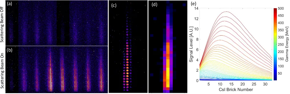
FIG. 2. (a) CsI scintillator raw data without the counter-propagating scattering beam. The signal is due to bremsstrahlung. (b) Raw data with the scattering beam on. The increase is due to gamma ray production through inverse Compton scattering of the electron beam with the counter-propagatingf /2 beam. (c) Single image of the CsI detector array obtained by imaging the scintillator with a camera. (d) The processed image with the individual pixels in each circle summed for spectral analysis. (e) Energy deposition curves of a monoenergetic photon beam impinging on a CsI detector array from 47 different Monte Carlo simulations performed in GEANT4.
matted data can be seen in Figure2(c) & (d).
B. GEANT4 Simulations
In order to analyze the data obtained from the crys-tal array, it is imperative to know how gamma rays will interact with CsI at various energies. Several 3D simula-tions were carried out in GEANT4 with various monoen-ergetic photon beams irradiating a slab of CsI, as shown in Figure 2(e), to generate response curves for the pho-ton energies relevant to this experiment. For this work, it was necessary to carry out 3D simulations due to sig-nificant amounts of side scatter and electron cascading that took place within the crystal array. Two dimsions were necessary to account for scattering and en-ergy transfer between neighboring CsI crystals and the third dimension was necessary to properly capture the geometry of the array so that light yield calculated by the simulations could be accurately compared to data. The incident photon energy in the simulations was var-ied from 0.1 MeV to 500 MeV with finer steps at low energy and larger steps at high energy. The lower limit was chosen because photons less than 0.1 MeV would not contribute any significant signal through the 9 mm thick steel detector housing. The simulations were stopped at 500 MeV as calculations indicate that the interaction would produce photons above this threshold in negligible quantities, well below the noise floor of the measurement.
C. Image Processing
The first step in analyzing the data files before the pix-els were summed together was to perform a background
subtraction. In this data, there are two types of back-ground that must be accounted for: the dark noise of the camera that provides a signal level of roughly 100
±2 counts even when the laser is turned off, and the background bremsstrahlung signal that appears when the scattering beam is turned off but electrons are still pro-duced. This signal is likely the result of stray electrons hitting the spectrometer magnets, shielding or chamber walls. These two types of background signal can be seen in Figure3(a) and (b).
To account for the dark noise of the camera, the region of the image containing CsI signal was cropped out and a background map was created from the remaining part of the image. This was done by performing a linear fit across each column of the remaining image and smooth-ing the result to generate a 1024×1024 “heat map” of the background so that areas of slightly higher or lower dark noise were properly accounted for. This dark noise background subtraction was done for each of the data shots and background bremsstrahlung shots.
[image:4.612.57.564.54.219.2]4
Brem Simulated Brem Data Data Signal
BG Signals
(a) (b) (c) (d)
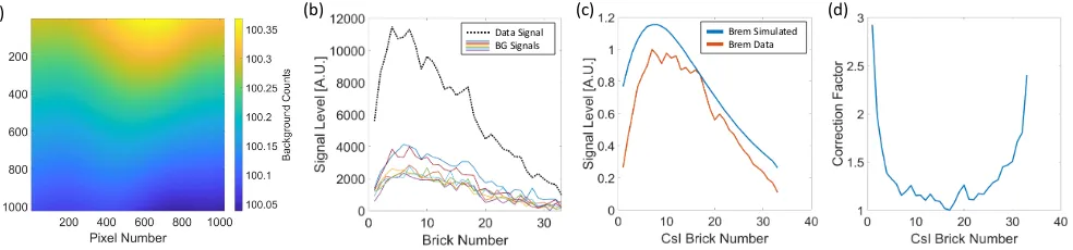
FIG. 3. (a) A “heatmap” of the dark noise background that was calculated and subtracted from each shot. (b) Seven different bremsstrahlung background curves plotted below an example data signal. The seven curves were subtracted from each data signal in the analysis. (c) Comparison of theoretical bremsstrahlung signal to actual bremsstrahlung data obtained during the experiment. The background data is normalized to the maximum value and the simulated background is normalized to the point of first overlap with the data. (d) Camera correction factor generated by dividing the theoretical signal by the actual signal.
Lastly, it was important to account for the
bremsstrahlung signal generated in addition to the gamma ray photons produced through the inverse Comp-ton scattering interaction. The level of this background varied from shot to shot as shown in Figure2(a). Since it was impossible to know the exact level of non-inverse Compton gamma photons that contributed to the signal on every shot, this variable background was a source of error in the spectrum calculations. Further discussion of how the background was accounted for in the calculations is covered in SectionII E.
D. Correction Factor
During the experiment, calibration shots were per-formed by colliding the electron beam with a 9 mm thick piece of lead to measure the CsI signal resulting from a bremsstrahlung interaction. By comparing this signal to a simulated bremsstrahlung signal, it was possible to con-firm the reliability of the detector and determine if the CsI detector system responded as expected to the gamma ray beam. The signal comparison between the data and simulation can be seen in Figure3(c). The curves in this figure were generated by summing the signal of the CsI crystals down the columns to compare the total signal generated from experiment and simulation.
The theoretical bremsstrahlung signal was generated in GEANT4 by simulating the collision of an electron beam with a energy spectrum typical of the experiment with a 9 mm thick piece of lead. The resulting gamma ray beam interacted with a simulated detector to generate a CsI signal that could be compared with experimental signal. This comparison required the assumption that the detector response to bremsstrahlung radiation was very similar in shape for slightly varying electron spectra; this was verified through simulation and the experimental data. The difference between the actual signal and the theoretical signal indicated a problem with the detector, most notably in the first few and last few crystals. The
discrepancy between the measured bremsstrahlung sig-nal and the theoretical sigsig-nal along with verification of consistent CsI signal resulted in the creation of a sin-gle “camera correction” curve to be applied to all the data during the analysis; this correction is shown in Fig-ure3(d).
Along with correcting for the low light yield of the first and last few crystals, likely caused by poor crys-tal quality or inadequate capture of the CsI fluorescence due to the optics used for the camera (vignetting), it was important to correct for the non-uniformity of the crystal light yield. This ensured that the calculations were performed with a more accurately represented sig-nal curve. While the correction factor accounted for the shape of the signal along with some of the inherent non-uniformity, it was not complete and applying a smooth fit to the noisy data to obtain an ideal signal level could fully account for the residual noise. The simulated sig-nal in Figure 3(c) and the detector response curves in Figure2(e) indicate that the CsI signal should not vary from one crystal to the next as significantly as the experi-mental data indicates. The non-uniformity of the crystal light output was a source of error in the spectral calcu-lations as the noise allowed for several different best-fit lines to the same data.
For this work, we defined a few different parameters to aid in describing the quality of the fit. We define
theexperimental error as the standard deviation of the
difference between the measured dataSi and the smooth best fit curvefi, normalized by the summed signal level of the best fit curve,
Experimental Error =σ(SPi−fi) ifi
. (1)
[image:5.612.64.556.52.167.2]The best fit to the data was calculated by performing 6th, 7th, and 8th degree polynomial fits to the data and
choosing the curve with the best fit quality.
E. Iterative Calculations
An algorithm was written to calculate the input spec-trum that would match the data after simulating its in-teraction with the CsI array in GEANT4. The algorithm is similar to the YOGI code1,2 in which the spectrum is
calculated by introducing perturbations to an assumed exponential shape and checking the result of those per-turbations against the data curve. The form of the ex-ponential spectrum used in this algorithm is
dN
dE =A×E
−2/3×e− E
Ecrit . (2)
This form was the best fit equation to a spectrum pro-duced by a simulated inverse nonlinear Compton scatter-ing interaction21,24. In this equation,Ais the amplitude
of the spectrum, E is the photon energy, and Ecrit is a characteristic energy of the spectrum with 49% of the photon energy radiated belowEcritand the mean photon energy isEcrit/3.
A single gamma ray of energyE incident on the scin-tillator array will generate a responseρi(E), wherei de-notes the ith element in the array. The response of the CsI scintillator to deposited energy is linear, and so for a distribution of photons, the total signal measured on the scintillator array will be Si = R
∞
0 ρi(E)f(E)dE, where
f(E)dE is the number of photons with energies in the rangeE toE+dE.
Using GEANT4, we calculated responses for a series of photon distributions fcalc(E, Ecrit) = (dN/dE)/A, given
by Eq. 2, over a range of values ofEcritj , wherejis thejth
calculated spectrum. This yielded a series of simulated scintillator array signals
Σi(Ecritj ) =
Z ∞
0
ρicalc(E)fcalc(E, Ecritj )dE
=
Z ∞
0
ρicalc(E)E
−2/3exp − E
Ecritj
!
dE ,(3)
whereρi
calc(E) is the simulated response function, i.e. the
signal calculated in the simulated array by GEANT4 for a photon of energyE.
For the iterative calculation of the experimental spec-trum, starting with a guessed spectrum fcalc(E, Ecrit0 ),
the measured signal for a particular shot Si was com-pared with Σi(Ecrit0 ). A new guessed spectrum was
cal-culated by adding a random perturbation to Aj and Ecritj to generate new spectra with Aj+1 = Aj +δA,
Ecritj+1=E
j
crit+δEcrit for a number of perturbations in a
generationj, and the quality of the fit between the data
and calculated signal was characterized by theR2 value
R2= 1−
P
i(Si−Σi)2 P
i(Si−S¯i)2
, (4)
where ¯Si is the average ofSi. The valuesAj+1andEcritj+1
corresponding to the largest R2 value for the different
perturbations in the generation was then taken as the starting point for the next iteration and when the algo-rithm converged, the spectrumAj+1E−2/3exp
− E
Ejcrit+1
was taken to best represent the real photon spectrum. Similar to the experimental error, we define the calcu-lated error as
Calculated Error =σ(ΣPi−fi| ifi
, (5)
as illustrated in Figure4(b). The calculated signal comes from the iterative perturbation method described previ-ously and the ideal signal is the same signal as listed in Equation (1). Characterizing the fit of the calculated signal this way is useful because it can be compared di-rectly to the inherit error of the detector through the experimental error. An example of the calculated signal with the raw data and the calculated spectrum can be seen in Figure5(a) – (f).
As mentioned previously, determining the proper back-ground subtraction was challenging in this work as it had a significant effect on the resulting fit and spectrum. Starting with a [1×33] vector of data,s, having the cor-rection factor applied, seven different background shots, b, were subtracted such thats′
is a matrix derived from the concatenation of the vectors s−b of size [7×33]. Now there are seven different data curves for each shot, each with its own potential background subtraction. The fitting algorithm was run to calculate a critical energy (Ecrit), amplitude (A), fit quality (R2), and ratio be-tween the first point of the data and first point of the fit for each of the seven options. Seven background shots were chosen as they were consecutive shots that were rep-resentative of the potential background produced by the wakefield beam only. The CsI signal of these seven shots can be found in Figure 4 in Cole et al24. An example of
these numbers for a data shot is shown in TableI. The relationship between the first point of the data and the fit is important as the fit quality of the first few points has a much higher effect on the calculated critical energy than the last few points. Figure4(c) shows that when the ratio of the first point of the data to the first point of the calculated signal is greater than 1, the algorithm over-estimates the critical energy and when it is less than 1, the critical energy is under-estimated. Figure4(d) shows that the fit quality of the last point does not affect the critical energy.
To define which background subtraction was the “cor-rect” subtraction, the R2 value was averaged with the
6
(c) (d)
(a) (b)
FIG. 4. (a) Comparison between the data signal and the ideal signal obtained by a best fit. The red arrows show some of the amplitude differences that were measured in calculating the experimental error. (b) Comparison between the calculated signal and the ideal signal for the same shot as (a). The difference between the two signals is used to calculate the relative error. (c) Relationship between the critical energy and the ratio of the last data point and last point of the calculated signal. (d) Relationship between the critical energy and the ratio of the first data point to the first point of the calculated signal. Each color ‘×’ represents the 7 background
subtractions of a single shot.
Parameter BG 1 BG 2 BG 3 BG 4 BG 5 BG 6 BG 7
R2 0.997 0.992 0.986 0.989 0.988 0.993 0.969
FPR 0.991 1.003 1.035 1.030 0.977 0.991 1.015
Ec[MeV] 21.22 52.26 98.63 44.71 60.12 50.61 33.84
[image:7.612.317.562.51.409.2]A 2.11 1.43 0.98 1.68 1.33 1.47 1.62
TABLE I. Table showing the values returned by running the fitting algorithm to the seven background subtracted data curves. The results show that the fit with the highestR2does not always correspond to the fit with the highest first point ratio (FPR), which is why both needed to be considered in choosing the background that resulted in the best fit.
background subtraction. Averaging the two values to-gether proved to be the best way to equally weigh each of the two measurements. This method took into account both the quality of the fit and accuracy of the first point fit as it was possible to have background subtraction with a high fit quality overall but poor fit on the first point resulting in a heavily over- or under-estimated critical energy.
Upon determining the correct background subtraction for each shot, a noise analysis was performed to
deter-(a) (b)
(c) (d)
(e) (f)
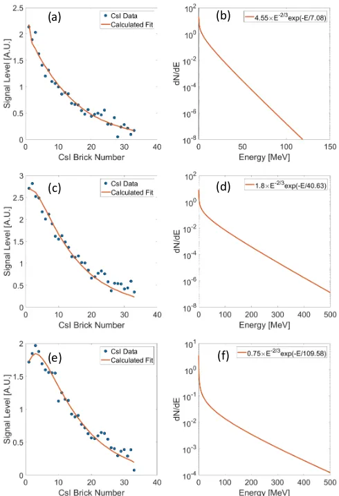
FIG. 5. Data and calculated fit plotted with corresponding spectra. The data obtained from the CsI detector is marked with the blue dots and the calculated fit is plotted as the solid line among the dots. (a) + (b) Example of a low critical en-ergy fit and spectrum ofEcrit= 7.08 MeV. (c) + (d) Example of a moderate critical energy fit and spectrum withEcrit= 40.63 MeV. (e) + (f) Example of a high critical energy fit and spectrum withEcrit= 109.58 MeV.
mine the sensitivity of the critical energy calculations to noisy data. For each shot, the experimental error was used as the amplitude metric and random noise was added to each bin of the ideal signal ranging from1/2to
2×the experimental error. Once new signal was
[image:7.612.55.293.52.276.2] [image:7.612.54.299.435.513.2]III. RESULTS
Comparing thecalculated errorto theexperimental er-ror is a good way to quantify the quality of the fit with respect to the original data. To determine how well the calculated signal fits the data, therelative error is
Relative Error = σ(Σi−fi)
σ(Si−fi) . (6)
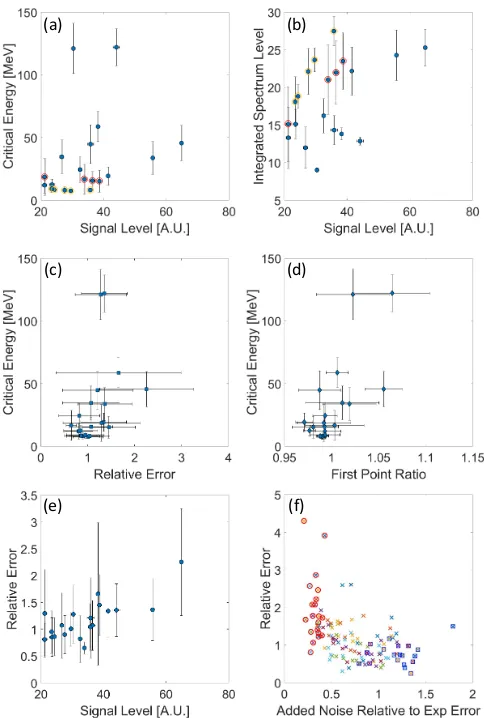
The integral of the ideal signal (from the denominator) cancels when these two errors are divided by one another. Figure 6 compares the critical energy, detector signal level (the summation of the ‘counts’ in each crystal), in-tegrated spectrum level and fit quality parameters to one another. In (a) and (b) of the figure, are plots that de-scribe the physics of the inverse Compton scattering in-teraction and in (c) - (f) are plots that describe the suc-cess of the iterative algorithm. Figure 6(a) shows the critical energy plotted against the signal level of the de-tector. There appears to be a very weak positive trend between the CsI signal level and the calculated critical energy if a few of the higher, outlier signals are ignored. This is somewhat to be expected as a more successful overlap of the electron beam with the scattering laser should produce more photons and higher energy pho-tons. If the trend were stronger, it would indicate that the number of electrons interacting with the laser pulse on each shot remained constant. The rather weak trend, indicates that the number of electrons scattered by the laser on each shot was not constant, likely due to the charge variability in the electron beam and fluctuations in the laser-electron beam overlap. In Figure 6(b), the relationship between the integrated signal on the detec-tor and integrated reconstructed spectrum is compared. If the critical energy was the same for all spectra, all the points on this plot would lie on a straight line. The increasing trend is expected, however, because higher en-ergy photons deposit more signal into the detector than lower energy photons, (see Figure 2(e)). For shots with the same critical energy, there is a direct, linear relation-ship between number of photons and CsI signal level that can be extracted. The highlighted shots in Figure 6(a) and (b) show some of these shots with a similar critical energy.
The trends shown in Figure6(c) - (f) are more telling of the fitting algorithm than the physics of the interaction. In (c), the critical energy is plotted against the first point ratio for the noise analysis data as opposed to the back-ground subtracted data as is the case with Figure 4(a). This now shows that the relationship between the first point and the critical energy is much weaker and that most of the points are very close to unity. This indicates that the critical energy measurement is more trustworthy and the over- or under-estimation is within a reasonable error. The plot in (d) shows that there is no relationship between critical energy and relative error. This is desir-able as a relationship between the energy of the photons and the fit quality would imply that there were errors
(c) (d)
(e) (f)
(a) (b)
FIG. 6. Measurements of various trends across 20 shots. (a) The integrated signal level on the CsI detector plotted against the measured critical energy. (b) Shows the relationship be-tween the CsI detector signal level and the area under the curve of the calculated spectrum. (c) The relationship be-tween the first point ratio and critical energy after the correct background was subtracted. (d) Shows there is not a rela-tionship between the relative error (defined in Section II E) and the critical energy. (e) Relative error plotted against the detector signal level showing a slight positive trend. (f) Rela-tive error plotted against the added noise. The minimum and maximum added noise are highlighted with red circles and blue squares respectively.
[image:8.612.318.560.55.414.2]8
the relationship between the relative error and the added noise. As expected, the relative error decreases with in-creasing noise because higher noise means higher exper-imental error, which is the denominator of Equation 6. The highlighted red and blue points show the minimum and maximum added noise respectively. As expected, the minimum noise resulted in higher discrepancies between the calculated fit quality and the ideal signal.
IV. CONCLUSIONS
In conclusion, we developed a CsI gamma ray spec-trometer by placing an array of CsI crystals parallel to the gamma beam propagation direction in order to mea-sure penetration depth. The meamea-surements of CsI scin-tillation were made with the counter-propagating beam turned on and off as shown in Figure2. The figure shows that on average, the CsI bricks produced a higher light yield when the scattering beam was turned on indicating that the counter-propagating laser pulse caused the cre-ation of high energy gamma rays. Since the increase in signal above the background bremsstrahlung signal was the result of only turning on the scattering beam, we are confident that the source of gamma rays is from inverse Compton scattering. With many of the shots producing spectra with critical energies higher than 30 MeV, this represents highest energy gamma rays produced through inverse Compton scattering on an all-optical source to date.
We were able to use this detector as a spectrometer by perturbing an assumed exponential spectrum and us-ing GEANT4 simulations to match the detector response to the data30,31. The resulting fit between the data and
signal produced by calculated spectra was overall very good with the majority of the shots having a lower er-ror than the inherent erer-ror of the CsI fluorescence. With GEANT4 simulations performed in advance, this detec-tor setup along with the algorithm could be implemented in future experiments as a gamma ray spectrometer ca-pable of producing a spectrum on a shot-by-shot basis. To improve the detector design, it would be beneficial to change the 9 mm thick steel side plate to a thinner, lower-Z material to mitigate the absorption of gamma rays in the housing. It would also be helpful to remove the faceplate of the detector that restricts the fluores-cence to circular holes so that each crystal’s fluoresfluores-cence can be captured entirely.
V. ACKNOWLEDGEMENTS
We acknowledge funding from the U.S. NSF CA-REER Grant No. 1054164, U.S. DOD under Grant No. W911NF-16-1-0044 and the U.S. DOE under Grant No. DE-NA0002372. EPSRC Grants No. EP/ M018555/1, No. EP/M018091/1, and No. EP/M018156/1, STFC
Grants No. ST/J002062/1 and No. ST/P000835/1,
Horizon 2020 funding under the Marie Sklodowska- Curie Grant No. 701676 and the European Research Council (ERC) Grant Agreement No. 682399, the Knut & Alice Wallenberg Foundation, the Swedish Research Council, Grants No. 2012-5644 and No. 2013-4248, Simulations were performed on resources provided by the Swedish National Infrastructure for Computing at the HPC2N. We would like to thank the CLF for their assistance in running the experiment.
REFERENCES
1G. Carlson, D. Fehl, and L. Lorence, “A differential absorption
spectrometer for determining flash x-ray spectra,” Nuclear In-struments and Methods in Physics Research Section B: Beam Interactions with Materials and Atoms, vol. 62, no. 2, pp. 264– 274, 1991.
2S. G. Gorbics and N. Pereira, “Differential absorption
spectrome-ter for pulsed bremsstrahlung,”Review of scientific instruments, vol. 64, no. 7, pp. 1835–1840, 1993.
3K. A. J. A. H. A. P. A. M. A. D. A. S. B. G. B. e. a. S. Agostinelli,
J. Allison, “Geant4a simulation toolkit,”Nucl. Instrum. Methods Phys. Res., Sect. A, vol. 506, p. 250, 2003.
4C. Geddes, C. Toth, J. Van Tilborg, E. Esarey, C. Schroeder,
D. Bruhwiler, C. Nieter, J. Cary, and W. Leemans, “High-quality electron beams from a laser wakefield accelerator using plasma-channel guiding.,”Nature, vol. 431, no. 7008, pp. 538–541, 2004.
5J. Faure, Y. Glinec, A. Pukhov, S. Kiselev, S. Gordienko,
E. Lefebvre, J.-P. Rousseau, F. Burgy, and V. Malka, “A laser-plasma accelerator producing monoenergetic electron beams.,”
Nature, vol. 431, no. 7008, pp. 541–544, 2004.
6S. Mangles, C. Murphy, Z. Najmudin, A. Thomas, J.
Col-lier, A. Dangor, E. Divall, P. Foster, J. Gallacher, C. Hooker, D. Jaroszynski, A. Langley, W. Mori, P. Norreys, F. Tsung, R. Viskup, B. Walton, and K. Krushelnick, “Monoenergetic beams of relativistic electrons from intense laser-plasma inter-actions.,”Nature, vol. 431, no. 7008, pp. 535–538, 2004.
7F. Albert and A. G. Thomas, “Applications of laser wakefield
accelerator-based light sources,”Plasma Physics and Controlled Fusion, vol. 58, no. 10, p. 103001, 2016.
8P. Lale, “The examination of internal tissues, using gamma-ray
scatter with a possible extension to megavoltage radiography,”
Physics in medicine and biology, vol. 4, no. 2, p. 159, 1959.
9R. Clarke and G. Van Dyk, “Compton-scattered gamma rays
in diagnostic radiography,” in Medical Radioisotope Scintigra-phy. VI Proceedings of a Symposium on Medical Radioisotope Scintigraphy, 1969.
10K. T. Phuoc, S. Corde, C. Thaury, V. Malka, A. Tafzi, J.-P.
God-det, R. Shah, S. Sebban, and A. Rousse, “All-optical compton gamma-ray source,”arXiv preprint arXiv:1301.3973, 2013.
11S. Chen, N. Powers, I. Ghebregziabher, C. Maharjan, C. Liu,
G. Golovin, S. Banerjee, J. Zhang, N. Cunningham, A. Moorti,
et al., “Mev-energy x rays from inverse compton scattering with laser-wakefield accelerated electrons,” Physical review letters, vol. 110, no. 15, p. 155003, 2013.
12G. Sarri, D. Corvan, W. Schumaker, J. Cole, A. Di Piazza,
H. Ahmed, C. Harvey, C. H. Keitel, K. Krushelnick, S. Man-gles, et al., “Ultrahigh brilliance multi-mev γ-ray beams from
nonlinear relativistic thomson scattering,” Physical review let-ters, vol. 113, no. 22, p. 224801, 2014.
13W. Yan, C. Fruhling, G. Golovin, D. Haden, J. Luo, P. Zhang,
14V. Malka, J. Faure, Y. A. Gauduel, E. Lefebvre, A. Rousse,
and K. T. Phuoc, “Principles and applications of compact laser-plasma accelerators,”Nat Phys, vol. 4, pp. 447–453, June 2008.
15T. Fuchs, H. Szymanowski, U. Oelfke, Y. Glinec, C. Rechatin,
J. Faure, and V. Malka, “Treatment planning for laser-accelerated very-high energy electrons,”Physics in Medicine & Biology, vol. 54, no. 11, p. 3315, 2009.
16Y. Glinec, J. Faure, L. Le Dain, S. Darbon, T. Hosokai, J. Santos,
E. Lefebvre, J.-P. Rousseau, F. Burgy, B. Mercier,et al., “High-resolutionγ-ray radiography produced by a laser-plasma driven
electron source,”Physical review letters, vol. 94, no. 2, p. 025003, 2005.
17F. Albert, S. Anderson, G. Anderson, S. Betts, D. Gibson,
C. Hagmann, J. Hall, M. Johnson, M. Messerly, V. Semenov, M. Shverdin, A. Tremaine, F. Hartemann, C. Siders, D. Mc-Nabb, and C. Barty, “Isotope-specific detection of low-density materials with laser-based monoenergetic gamma-rays,”Optics Letters, vol. 35, no. 3, pp. 354–356, 2010.
18R. T. Klann, J. Shergur, and G. Mattesich, “Current state of
commercial radiation detection equipment for homeland security applications,” Nuclear Technology, vol. 168, no. 1, pp. 79–88, 2009.
19C. Moss, C. Hollas, G. McKinney, and W. Myers,
“Compari-son of active interrogation techniques,” inIEEE Nuclear Science Symposium Conference Record, 2005, vol. 1, pp. 329–332, IEEE, 2005.
20A. G. R. Thomas, C. P. Ridgers, S. S. Bulanov, B. J. Griffin, and
S. P. D. Mangles, “Strong radiation-damping effects in a gamma-ray source generated by the interaction of a high-intensity laser with a wakefield-accelerated electron beam,”Phys. Rev. X, vol. 2, p. 041004, 2012.
21T. G. Blackburn, C. P. Ridgers, J. G. Kirk, and A. R. Bell,
“Quantum radiation reaction in laser˘electron-beam collisions,”
Phys. Rev. Lett., vol. 112, p. 015001, Jan 2014.
22E. Nerush, I. Kostyukov, A. Fedotov, N. Narozhny, N.
Elk-ina, and H. Ruhl, “Laser field absorption in self-generated electron-positron pair plasma,”Physical Review Letters, vol. 106, p. 035001, 2011.
23N. Elkina, A. Fedotov, I. Kostyukov, M. Legkov, N. Narozhny,
E. Nerush, and H. Ruhl, “QED cascades induced by circularly polarized laser fields,”Physical Review Accelerators and Beams, vol. 14, p. 054401, 2011.
24J. M. Cole, K. T. Behm, E. Gerstmayr, T. G. Blackburn, J. C.
Wood, C. D. Baird, M. J. Duff, C. Harvey, A. Ilderton, A. S.
Joglekar, K. Krushelnick, S. Kuschel, M. Marklund, P. McKenna, C. D. Murphy, K. Poder, C. P. Ridgers, G. M. Samarin, G. Sarri, D. R. Symes, A. G. R. Thomas, J. Warwick, M. Zepf, Z. Naj-mudin, and S. P. D. Mangles, “Experimental evidence of radia-tion reacradia-tion in the collision of a high-intensity laser pulse with a laser-wakefield accelerated electron beam,”Phys. Rev. X, vol. 8, p. 011020, Feb 2018.
25K. Poder, M. Tamburini, G. Sarri, A. Di Piazza, S. Kuschel, C. D.
Baird, K. Behm, S. Bohlen, J. M. Cole, D. J. Corvan, M. Duff, E. Gerstmayr, C. H. Keitel, K. Krushelnick, S. P. D. Mangles, P. McKenna, C. D. Murphy, Z. Najmudin, C. P. Ridgers, G. M. Samarin, D. R. Symes, A. G. R. Thomas, J. Warwick, and M. Zepf, “Experimental signatures of the quantum nature of ra-diation reaction in the field of an ultraintense laser,”Phys. Rev. X, vol. 8, p. 031004, Jul 2018.
26G. F. Knoll,Radiation detection and measurement; 4th ed.New
York, NY: Wiley, 2010.
27T. Ypsilantis and J. Seguinot, “Theory of ring imaging cherenkov
counters,” Nuclear Instruments and Methods in Physics Re-search Section A: Accelerators, Spectrometers, Detectors and As-sociated Equipment, vol. 343, no. 1, pp. 30 – 51, 1994.
28V. Sch¨onfelder and G. Kanbach,Imaging through Compton
scat-tering and pair creation, pp. 225–242. New York, NY: Springer New York, 2013.
29D. J. Corvan, G. Sarri, and M. Zepf, “Design of a compact
spec-trometer for high-flux mev gamma-ray beams,”Review of Scien-tific Instruments, vol. 85, no. 6, p. 065119, 2014.
30J. H. Jeon, K. Nakajima, H. T. Kim, Y. J. Rhee, V. B. Pathak,
M. H. Cho, J. H. Shin, B. J. Yoo, C. Hojbota, S. H. Jo, K. W. Shin, J. H. Sung, S. K. Lee, B. I. Cho, I. W. Choi, and C. H. Nam, “A broadband gamma-ray spectrometry using novel unfolding al-gorithms for characterization of laser wakefield-generated beta-tron radiation,”Review of Scientific Instruments, vol. 86, no. 12, p. 123116, 2015.
31J. H. Jeon, K. Nakajima, H. T. Kim, Y. J. Rhee, V. B. Pathak,