Expert knowledge elicitation using item response theory

(1)

This is a repository copy of

Expert knowledge elicitation using item response theory

.

White Rose Research Online URL for this paper:

http://eprints.whiterose.ac.uk/128337/

Version: Accepted Version

Article:

Andrade, JAA and Gosling, JP orcid.org/0000-0002-4072-3022 (2018) Expert knowledge

elicitation using item response theory. Journal of Applied Statistics, 45 (6). pp. 2981-2998.

ISSN 0266-4763

https://doi.org/10.1080/02664763.2018.1450365

This is an Accepted Manuscript of an article published by Taylor & Francis in Journal of

Applied Statistics on 16 March 2018, available online:

https://doi.org/10.1080/02664763.2018.1450365

Reuse

Items deposited in White Rose Research Online are protected by copyright, with all rights reserved unless indicated otherwise. They may be downloaded and/or printed for private study, or other acts as permitted by national copyright laws. The publisher or other rights holders may allow further reproduction and re-use of the full text version. This is indicated by the licence information on the White Rose Research Online record for the item.

Takedown

If you consider content in White Rose Research Online to be in breach of UK law, please notify us by

(2)

Expert knowledge elicitation using item response theory

J. A. A. Andradea _{and J. P. Gosling}b

a

Dept. of Statistics and Applied Mathematics, Federal University of Ceara, 60455-670, Fortaleza-Ce, Brazil.;b

School of Mathematics, University of Leeds, Leeds, LS2 9JT, UK.

ARTICLE HISTORY

Compiled February 15, 2018

Abstract

In an expert knowledge elicitation exercise, experts face a carefully constructed list of questions that they answer according to their knowledge. The elicitation process concludes when a probability distribution is found that adequately captures the experts’ beliefs in the light of those answers. In many situations, it is very difficult to create a set of questions that will efficiently capture the experts’ knowledge, since experts might not be able to make precise probabilistic statements about the parameter of interest. We present an approach for capturing expert knowledge based on item response theory, in which a set of binary response questions is proposed to the expert, trying to capture responses directly related to the quantity of interest. As a result, the posterior distribution of the parameter of interest will represent the elicited prior distribution that does not assume any particular parametric form. The method is illustrated by a simulated example and by an application involving the elicitation of rain prophets’ predictions for the rainy season in the north-east of Brazil.

Keywords: Subjective probability, item response theory, latent trait, prior information, nonparametric elicitation, rain prophets.

1. Introduction

In Bayesian analyses, we combine data and prior information in order to obtain the posterior distribution about the quantities of interest. Prior knowledge is typically represented by some probability distribution that will encapsulate all we know about the quantity before observing the data. When the prior information is obtained from experts, we need some robust and defensible method to translate their knowledge into a probability distribution. Therefore, expert knowledge has a substantial role to play in statistical inference and decision making (Cooke, 1991; Morgan and Henrion, 1992; O’Hagan et al., 2006) and has formed the basis of policy making for many years (Jungermann and Zeeuw, 1977; Morgan et al., 1984; Weible, 2008; Gosling et al., 2012). In order to have confidence in using expert judgements, structured expert knowledge elicitation (EKE) methods have been developed that are designed to improve reliability and improve transparency in the process. Given certain quantities of interest to a decision maker, EKE attempts to extract, as reliably as possible, relevant knowledge from experts. This process is usually conducted by a facilitator, a person responsible for the EKE process: their role is to design the questions, get

(3)

judgements from the experts and convert those judgements into a probability distribution. These tasks have many challenges: overconfidence on the experts’ part, experts’ lack of knowledge about probability and language barriers to name a few. An EKE protocol should aim to deal with the biases inherent in the process. O’Hagan et al. (2006) gives a detailed discussion about the problems faced in the application of EKE and some strategies that have been proposed for dealing with them.

There are EKE processes designed to deal with different situations that depend on the quantity of interest and the experts. We may have quantities that are easily measured: for example, the average level of cholesterol of a certain risk group. However, EKE becomes particularly difficult when the quantities of interest are not easily observed, in the sense that they cannot be directly measurable by any instrument. For instance, aspects related to the human mind are difficult to measure: depression in children (see De Roos and Allen-Meares, 1998), degree of xenophobia in a society, students abilities, and so on. These are called latent traits (or variables) that cannot be observed directly. Instead, we measure a quantity that provides a surrogate for the variable. In spite of the difficulties, in many real world problems, we do need to quantify latent variables.

From the Bayesian point of view, a latent variable is seen as a parameter in a statistical model; thus, EKE may need to be applied to obtain a prior probability distribution for a latent quantity of interest. However, it can be difficult to build an EKE protocol that is able to capture accurate quantitative judgements regarding an unobservable quantity (Kadane and Wolfson, 1998). Prob-abilistic inversion techniques have been used in the past to relate latent variables to observables, but these methods depend on the availability of a model of the real world process to reconstruct beliefs about the latent quantity (see Du et al., 2006; Kurowicka et al., 2010, for example).

A statistical tool that tries to make indirect measurements of latent traits is based upon item response theory (IRT) or latent trait theory. The method uses a dichotomous (or polytomous) response logistic (or probit) model that is associated with the latent quantities of interest. The way in which the latent trait and the items are related is that each positive answer to the items will indicate a high value of a latent trait. Although item response theory has been mostly applied in educational tests, it shares elements with logistic models and has a wide range of applications. There is a fundamental difference between logistic regression and IRT: in the first, the regressor variables are observed; whereas, in IRT, the regressor variables are non-observable parameters. Most of the applications of the theory are devoted to educational and psychological testing. For instance, in educational tests, IRT can help to calibrate questions so that a correct answer will signify certain abilities of some candidate. In this case, the probability of a correct answer for

candidate j (j= 1, ..., n) to the itemi(i= 1, ..., I) may be given by

P(Uij = 1|θj) =

1

1 +e−ψ(θj,ai,bi), (1)

where in the traditional IRT applications ψ(θj, ai, bi) = ai(θj −bi), Uij = 1 if the answer is

cor-rect and Uij = 0 otherwise, θj is the ability (latent trait which we want to measure), ai is the

discrimination parameter, which indicates the capability of the itemito discriminate between the

examinees with low and high ability; and bi is the difficulty parameter, which represents the

diffi-culty to answer correctly the item i. The model in (1) establishes that, for a given discrimination

and difficulty, a student with high abilityθj will have a higher probability of a correct answer. In

general, the scale of the ability and the item parameters are arbitrary.

(4)

ques-tionnaire (with a large number of questions) that will give some idea of the person’s height. For instance, the questions:

(1) “Do you need a chair to clean the top of your fridge?”

(2) “Do you need help to stow your hand luggage in an aeroplane?”

may help to capture the trait which represents the height of the person. See Hambleton et al. (1991) and Baker (2001) for a complete description of IRT.

In the present article, we propose an approach to EKE using item response theory in which we consider the quantity of interest in the EKE as the latent trait. In other words, the expert is asked to answer a questionnaire with dichotomous questions that are directly related with the parameter that we are to measure. Alternatives to this approach include the ranking of possibilities that can be translated into information about the quantity of interest and the use of imprecise probability models. Rank-based methods have been in use for many years to help derive subjective probability distributions (Smith, 1967; Kirkwood and Sarin, 1985). Recently, these methods have been applied in the context of horizon scanning for nanotechnologies (Flari et al., 2011) and the assessment of threats to animal health (Jaspersen and Montibeller, 2015). We propose the IRT-based approach as an alternative method when it is more straightforward to devise yes/no questions rather than pos-sibilities to rank. Of course, the relative utility of the two approaches will depend on the application area and the ability of the experts. A ranking method may be more suitable when the experts have a clear understanding of the proposed possibilities; in our application, the range of knowledge was such that the experts would not have a good appreciation of such scenarios. Imprecise probabilities have also been used to capture the ineffectiveness of traditional EKE techniques (Walley, 1996; O’Hagan and Oakley, 2004; Kriegler et al., 2009), but, in our approach, we can directly model the uncertainty using simple questions and straightforward probability modelling rather than adding an extra layer of mathematical complexity.

In Section 2, we define the problem and the IRT model to be used in the EKE. In particular, we

propose two models for parameters defined within the (0,1) interval. In Section 3, we illustrate the

method through a simulated example and we revisit the model proposed by Andrade and Gosling (2011) (using updated data) in which we compare the prior information obtained from Brazilian rain prophets by EKE and by IRT methods.

2. Expert elicitation through IRT

Let θ be a latent trait that we wish to capture expert knowledge about. In order to assess the

magnitude ofθ, suppose a dichotomous response questionnaire withI questions is created, in such

a way that, for several scenarios (events) directly associated with θ, an expert answer of “yes” will

indicate large values ofθ and “no” will be associated with small values. Let

Yij = (

1 if the jth expert responds “yes” to the ith question,

0 if the jth expert responds “no” to theith question,

for theI questions and nexperts. A linear IRT logistic model is of the form:

Pij =P(Yij = 1|θj, ai, bi) =

eψ(θj,ai,bi)

(5)

where i = 1, ..., I and j = 1, ..., n; the parameter θj represent the latent trait that led expert j

to respond “yes/no” to questions relating to θ; ai, bi are the item parameters, which are used to

assess the items in the same sense as in (1). In this set-up, we are allowing different experts to have

different beliefs aboutθusing the individualθj; combination of these separate beliefs to an overall

distribution forθ is discussed in Section 3.2.1.

In the following sections, we propose two models for θ that is constrained to be in (0,1). The

first model considers the item discrimination and difficulty parameters (ai, bi) which may be useful

to assess the IRT questionnaire itself, that is, in the case when it is possible, perhaps through a long ran repeated process, to judge the effectiveness of each item in capturing the latent trait. In contrast, the second model assumes that there is no information available about the discrimination and the difficulty involving the answer of the items.

2.1. Model with item parameters

The function ψ(θj, ai, bi) defines the type of IRT model. There are many plausible alternatives for

ψ(.), the most common are:ψ(θj, ai, bi) =ai(θj−bi) (two-parameter model),ψ(θj, ai, bi) = (θj−bi)

(one-parameter model or Rasch model) and the three parameters model, which takes in to account

the possibility that an expert, who believes in low values of θ, may answer “yes” to the item by

chance. All these models can be used in an EKE process. In the present work, we propose a new

functional form specially designed for a latent trait 0< θj <1:

ψ(θj, ai, bi) =ai

1

1−θj

− 1

θj −bi

, (3)

where the item parameters have similar interpretation as in the traditional models. We adapt the

interpretation to the EKE perspective where ai is the capability of the item i to discriminate

between those experts who believe in large values ofθj from those who believe in small values ofθj.

Also, the parameter,bi, will indicate the difficulty in responding positively to the itemiunder the

latent trait θj; that is, how unlikely is the scenario proposed by the itemi. For the purpose of this

work, the specific choice of the function in (3) provides a correspondence between the latent trait

θj and the probability of responding positively to some item i. For instance, for item parameters

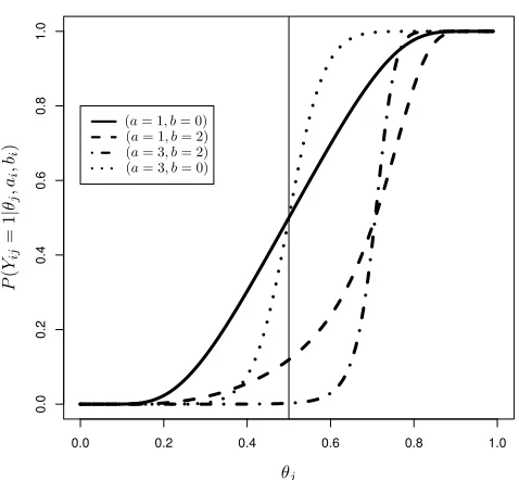
ai= 1 andbi = 0, a latent trait ofθj = 0.5 will lead to a probability of 0.5 of responding positively

to a certain item. In other words, an expert, who feels that the quantity of interest might be in the central point of the scale, will have a probability of 0.5 of answering “yes” to the proposed item. Of course, depending on the item parameters, this correspondence can be different, which is natural when we consider the nature (discrimination and difficulty) of each item.

The relation between the latent trait and item responses are shown in Figure 1. Large values ofai

mean that the item can efficiently discriminate between those experts who believe in large values

of θj and those who believe in low values of θj. In this model, the scale of ai must be positive,

otherwise the model would indicate that the probability of responding positively to some item

would be small when the expert holds a high latent trait θj. The parameterbi gives an indication

of how large the latent trait should be to respond positively to the item i, large values of bi will

require a high latent trait; that is, in order to respond “yes” to a given item, the expert should be

very confident ofθj being large.

(6)

0.0 0.2 0.4 0.6 0.8 1.0

0.0

0.2

0.4

0.6

0.8

1.0

θj

P

(

Yij

=

1

|

θj

,a

i

,bi

)

[image:6.595.180.419.101.322.2]

(a= 1, b= 0) (a= 1, b= 2) (a= 3, b= 2) (a= 3, b= 0)

Figure 1.: Item curve: solid line represents (ai = 1, bi = 0), compared to other

values of the parameters: (ai = 1, bi = 2) gives the curve of an item which is

more difficult to answer “yes”, (a = 3, b = 2) reflects a highly discriminative

and with high difficulty, whereas (a= 3, b= 0) expresses a highly discriminative

item but with low difficulty.

about the latent trait as well as the item parameters. Formally,

Yij|θj, ai, bi ∼Ber(Pij) (i.i.d.),

θj ∼πj, ai ∼pi, bi∼p∗i,

(4)

where Pij is given by (2) and πj, pi and p∗i are prior distributions, which should encode some

relevant information about the quantity of interest and the items characteristics (discrimination and difficulty). This information may be obtained from past studies or by eliciting qualitative information from experts involved in the formulation of the items. We assume independence among experts and local independence among the items; that is, given a certain ability of the experts, the responses are independent. Independence amongst items is not easy to assure because it depends on the IRT questionnaire itself. Some psychological strategies can be used to reduce dependence, such as possibly inserting other questions to avoid biased answers from one item to the next one. For further details of independence in IRT models, see Lee (2004) and Wang and Wilson (2005).

The likelihood function is given by

l(θ,a,b;y)∝ n Y

j=1

Y

i∈Ij

Pyij

ij (1−Pij)1−yij, (5)

where θ = (θ1, ..., θn), a = (a1, ..., aI), y = {yij}, b = (b1, ..., bI) and Ij is the set of indexes i

(7)

Due to the assumed inter-independence among experts and items, the posterior distributions will be given by

p(θ,a,b|y)∝ n Y

j=1 πj(θj)

I Y

i=1 pi(ai)

I Y

i=1 p∗

i(bi) n Y

j=1

Y

i∈Ij

Pyij

ij (1−Pij)

1−yij_,

fori= 1, ..., I and j= 1, ..., n.

In the traditional IRT tests, the model considers the discrimination and the difficulty aspects of each

item. The process of estimating (ai, bi) is called calibration, in which the items are calibrated by

submitting them to real word tests (pre-test), that is a large bank of items is sent to several schools and applied to the students, then based on their performance, the discrimination and the difficulty of each item are estimated; then, the estimation of the latent trait will take the point estimates of

ai andbi in consideration. Note that in order to achieve a good precision in the estimation process

we need both a large sample and a large number of items, that is we need as many respondents as possible for a good calibration and a large number of items in order to measure the abilities as accurately as possible. Note that this process can be very expensive and time demanding, also it carries a lot of uncertainty itself, due to the natural variance among students. Alternatively, as discussed by Fox et al. (2015), in a Bayesian framework, instead of treating the parameters as fixed quantities, we assign prior distributions to the item parameters. This eliminates the expensive stage of pre-testing the items and the prior distributions will express the item parameters (discrimination or difficulty) and the uncertainty about them. In addition, the introduction of informative prior information makes the IRT analysis less dependent on the sample size, which is a powerful tool since in many applications we have only a small number of respondents. The relation between sample size and the IRT estimation process in the Bayesian framework is explored in more detail by Torre and Hong (2010) and Matteucci et al. (2012).

2.2. Model without item parameters

Usually, the IRT theory may involve either three, two or one item parameters model, depending on the information available. In some situations, no prior information about any of the item parameters is available, this lack of information can be expressed by: (1) assigning diffuse prior distributions for the item parameters or (2) assuming the difficulty and discrimination are the same for all items. Note that in the first situation, although not knowing much about the difficulty and discrimination parameters, it is assumed that they may be different from one item to another, while the second scenario is more restrictive, the difficulty and discrimination parameters are the same for each item. Observe that the theory is flexible in allowing to build up different scenarios depending on the information available. In our case, we consider the second scenario, since in our application we preferred to assume that the item parameters are the same for all items. Thus we consider the a simplified version of the IRT logistic model (3), that is

Pj =P(Yj = 1|θj) =

e

1 1−θj−

1 θj

1 +e

1 1−θj−

1 θj

. (6)

With this model, the experts’ responses will not depend on the item parameters.

(8)

(correct or incorrect/NA), here the expert can respond “yes”, “no” or “NA” (no response), the latter is feasible since, in practice, the expert may not be able to respond to some of the questions. Nevertheless, the experts’ knowledge expressed in answers to the other questions should still be regarded as a valid source of information about the latent parameter. The missingness mechanism may vary with the application, we may have completely at random missingness (MCAR), where the missing answers does not follow any pattern; some missing data might depend only on some observed data (MAR) and; in a more complex setting the missingness follows some pattern involving both the observed and unobserved data (MNAR). A model of missingness could be incorporated to data model (Rubin, 1987), however this approach will require a rather deep knowledge of the data generating mechanism. In the proposed theory, missingness is assumed either MCAR or MAR, although the MAR assumption would require large datasets in order to be justified. It follows that the likelihood function is given by

l(θ;y)∝ Y j∈Ij

Pyj

j (1−Pj)1

−yj_, ₍₇₎

whereθ= (θ1, ..., θn) and Ij is the set of indexesj corresponding to the answered questions in the

questionnaire.

The posterior distributions will be given by

p(θ|y)∝ n Y

j=1 πj(θj)

Y

j∈Ij

Pyj

j (1−Pj)1

−yj_,

forj= 1, ..., n. Note that depending on the choices of the prior distributions the computation can become challenging. Albert (1992) proposed a general procedure for the two-parameters normal IRT model, using a data augmentation strategy to obtain the full conditionals to be used in the Gibbs sampling algorithm. Other works explored his ideas, for instance Albert and Chib (1993) considered polytomous responses, Albert (1998) showed how MCMC behaves for different sample sizes and the number of items. Several other studies consider Bayesian multidimensional IRT, giving special attention to the posterior computation: Fox and Glas (2001), Fu et al. (2009) and Sheng and Wikle (2009), to cite a few. Roughly speaking, these works provide methods to efficiently implement the MCMC algorithms in rather complex multivariate settings. For instance, Fox et al.

(2015) simulate quite efficiently from the posterior distribution using WinBUGS in several complex

models such as unidimensional and multilevel models. In the present paper, we consider EKE for a single parameter, which will be approached with the unidimensional IRT theory, which is relatively

straightforward to implement in common MCMC packages. In particular,WinBUGS/OpenBUGS have

a great variety of distributions available that are suitable for using as prior distributions of the latent trait (quantity of interest) and the item parameters.

3. Examples

(9)

3.1. Simulated example

We consider a problem of eliciting prior information concerning some parameter 0 < θ < 1. We

suppose an IRT questionnaire ofI = 20 questions is proposed toJ = 10 experts. The questionnaire

is built in a such way that, for each answer 1 indicates higher values ofθ. The aim of this example is

to assess the relation between the set of answers of the experts and posterior distribution resulting

from the IRT method, that is we want to obtainp(θ|y) which will play the role of the elicited prior

distributionp(θ). We consider Model (4), with Pij (j= 1, ...,10 andi= 1, ...,20) given by (2) and

ψ(θj, ai, bi) (j= 1, ...,10 andi= 1, ...,20) given by (3). We assignθ∼Uniform(0,1), ai ∼Ga(3,5)

(iid) andbi ∼Ga(2,4) (iid) (i= 1, ...,20). The posterior distribution will be given by

p(θj, ai, bi|y)∝ayi

1

1−θj

− 1

θj −bi

y

1−ai

1

1−θj

− 1

θj −bi

n−y

a2_ie−5ai_b

ie−3bi, (8)

where y vector of valid answers (0 or 1), y = P

i P

jyij and n is the number of valid answers.

We assume that the discrimination and the difficulty parameters are independent and identically

distributed according to some gamma distribution, respectively ai ∼ G(3,5) and bi ∼G(2,4) ∀i,

thus all the items have the same law of discrimination and difficulty. Then we simulate different sample scenarios by changing the number of “Yes”, “No” and “NA” responses, thus we can assess

the impact (location and dispersion) in the posterior distributions ofθaccordingly to the proportion

of “Yes”, “No” and “NA” responses.

Given that (8) is not tractable analytically, we used the OpenBugs code of Appendix A to obtain

the posterior distributions for each set of answers of the expert, denoted by the percentages of

(1,0,NA).

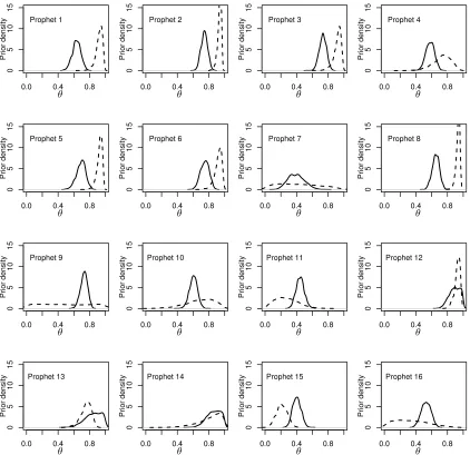
The derived prior distribution and the mean and standard deviation in each hypothetical set-up (Figure 2) indicate that in the case of 100% of “yes” answers (Expert 1) the prior obtained will be concentrated very close to 1 and the standard deviation is relatively small, that is the expert

feels that θwill likely be high and he/she is quite certain about it. In contrast, all “no” responses

will yield a prior distribution close tozero with some higher variance. The presence of many “NA”

answers greatly increases uncertainty about theta, either because the expert was in doubt about the items or could not respond to them (Experts 9 and 10, Fig. 2). Note that this presents well the idea of elicitation, since if the questionnaire fails to collect a valid answer we loose some piece

of information about θ. For example, Expert 6 answered 50% of “yes” and left unanswered 50% of

the questions, in this case there is still evidence for high values ofθhowever with a larger variance.

Expert 3 answered equally “yes” and “no”, which yielded a prior distribution around 0.71, note that although we have the same proportion of “yes” and “no”, the discrimination and the difficulty

parameters are playing some role inPij, that is a response “yes” contributes more for higher values

of θthan a response “no” contributes for lower values of θ.

In summary, the model is converting different experts’ set of answers into prior distributions. The

function in (3) is proposed to deal with parameters defined in (0,1), other expressions forψcan be

proposed, depending on the quantity of interest. The item parameters, which should express the discrimination capability and the difficulty of each item, will have a direct impact on the final prior

distributions since items with large power of discrimination will increase the probability Pij if the

(10)

0.0 0.2 0.4 0.6 0.8 1.0 0 5 10 20 Pr ior density

Expert 1 − (100%,0%,0%)

0.0 0.2 0.4 0.6 0.8 1.0

0 5 10 20 Pr ior density

Expert 2 − (75%,25%,0%)

0.0 0.2 0.4 0.6 0.8 1.0

Expert 3 − (50%,50%,0%)

0.0 0.2 0.4 0.6 0.8 1.0

Expert 4 − (25%,75%,0%)

0.0 0.2 0.4 0.6 0.8 1.0

Expert 5 − (0%,100%,0%)

0.0 0.2 0.4 0.6 0.8 1.0

Expert 6 − (50%,0%,50%)

0.0 0.2 0.4 0.6 0.8 1.0

Expert 7 − (50%,25%,25%)

0.0 0.2 0.4 0.6 0.8 1.0

Expert 8 − (25%,50%,25%)

0.0 0.2 0.4 0.6 0.8 1.0

Expert 9 − (0%,50%,50%)

0.0 0.2 0.4 0.6 0.8 1.0

Expert 10 − (0%,25%,75%)

[image:10.595.84.504.81.535.2]

θθ θθ θθ θθ θθ θθ θθ θθ θθ θθ mean=0.9694 sd=0.0247 mean=0.8410 sd=0.0470 mean=0.7108 sd=0.0662 mean=0.5187 sd=0.0814 mean=0.1407 sd=0.0943 mean=0.9040 sd=0.0659 mean=0.7896 sd=0.0689 mean=0.6215 sd=0.0914 mean=0.1496 sd=0.0980 mean=0.1795 sd=0.1153

Figure 2.: Experts’ prior densities for each set of answers: percentages of (1,0,NA). A

large number of “Yes” answers will draws the prior distribution closer toone, whereas a

large number of “No” answers will bring it closer to zero. A large number of “NA” will

be characterised by a greater dispersion.

3.2. Application: quantifying the beliefs of rain prophets

(11)

forecasting very difficult for meteorologists. In this context, the figures popularly known as rain prophets, although they reject this designation, have a reputation for accurate seasonal weather prediction. The prophets make claims about being able to make predictions based on the behaviour of nature: that is plants, animals, stars, winds, and so on. For instance, the way ants clear their nests is associated with water flow, also frogs hibernation period seems to predict the soil humidity. Taddei (2005) reviews a wide range of natural phenomena observed by the rain prophets for use in their predictions.

In the model proposed by Andrade and Gosling (2011), the experts were the rain prophets and the quantity elicited was the probability of a good rainy season. The elicitation task was particularly challenging due to the prophets’ lack of familiarity with probability, ambiguity in qualitative state-ments, dialectal language, etc.. In a more general context, Burgman (2015) provides some further discussion about the problems found using expert’s knowledge and how to approach them in the decision process. Formally, Andrade and Gosling (2011) proposed an elicitation setting specific for

the rain prophets in which the quantity of interest was θ: the probability of a good rainy season.

This was defined by the prophets themselves as “wet ground throughout the season”. In this EKE method, several important biases were considered such as illiteracy, the dialectal language, lack of knowledge about probability and great uncertainty. The procedure tried to embrace these issues, yielding a probability (prior) density for each prophet, which represented his knowledge about the forthcoming rainy season. Thus, their opinions were elicited with the aim that the local population could have a clearer idea about the predictions. For instance, we could have, in the local press, statements such as “according to the rain prophets, the probability of having a good rainy season is 64%” (Andrade and Gosling, 2008), indicating their beliefs in a way that could be understood by the general public.

In the present paper, θ is treated as a latent trait from the IRT perspective. In 2012, during the

annual prophets’ meeting, which takes place in the first week of January, we applied the same elicitation procedure of Andrade and Gosling (2011), in order to obtain for each prophet the prior

distributions for θ, the probability of a good rainy season. At the same meeting, we applied a

dichotomous response questionnaire to the same prophets as suggested in Section 2. In the EKE method the parameter of interest is the probability of a good rainy season, while in the IRT method

θis a latent trait which cannot be interpreted as such, but a quantity which indicates how confident

in a (0,1) range the rain prophet is about the forthcoming rainy season. This will allow us to make

a rough comparison between the probability of a good rainy season with the latent trait which indicates how much the prophet the prophets’ beliefs.

The IRT procedure is useful since we can use a questionnaire with several simple questions which

will be answered with “yes”, “no” or non-response, where an answer “yes” is set as one and will

indicate a larger value for the latent trait of a good rainy season, and zero otherwise. Note that

from the prophet’s point of view, answering “yes” or “no” is much easier than trying to figure out the possible values of the parameter and the uncertainty associated with it. The questionnaire was based on anthropological studies by Taddei (2005), who gives details regarding which natural phenomena the prophets observe. Questions relate to the actual elements of the local ecosystem that the respondents observed during the four months before the meeting. The questions are listed in Appendix B.

All the aspects covered in the questions are closely related to a good rainy season according to

studies of the rain prophets, and every positive answer will indicate a higher latent trait θ. There

(12)

embraces only the valid responses.

As mentioned before, constructing prior distributions for the item parameters involves some effort, since a specialist needs to express their opinions concerning the discrimination and the difficulty about each item through a probability density. In our example, there are no specialists to assess the proposed items, because this would require a long term experience about the efficiency and the difficulty of each item in predicting a good rainy season. Therefore, we consider a simplified version

of the IRT logistic model (3), where Pij =Pj. Thus, the prophets’ responses will depend only on

their latent trait of the a good rainy season. We rewrite model (4) as

Yj|θj ∼ Ber(Pj) ind,

θj ∼ Uniform(0,1),

(9)

where j = 1, ...,16, Pj is given by (6). In this way, the posterior distribution pj(θj|y) = pj(θj)

(j = 1, ...,16) will represent the uncertainty about the rainy season of each prophet.

In order to compare the elicited prior distributions obtained from the EKE and IRT methods, we consider the same EKE procedure adopted by Andrade and Gosling (2011): that is, we assume that

the prior information about eachθj have Kumaraswamy distributions with parameters obtained by

the elicitation procedure, that is we elicit from the rain prophets the mode and the variance of the

Kumaraswamy distribution, then we obtain its parameters. The information carried byπj(θj) about

θj (j = 1, ...,16) provided by that EKE method will be compared with the latent trait evidences

obtained by the IRT questionnaire (applied to the same prophet).

3.2.1. Results

We used the packageOpenBugsto extract a sample from the posterior distribution for the θj (the

OpenBugscode is in Appendix A). We compare (Figure 3) the prior distributions obtained by the EKE (resulted from the same procedure of Andrade and Gosling, 2011) with the IRT method (Model (9)). By comparing the modes, the EKE and IRT methods seem to capture approximately the same prior knowledge of some prophets (4, 12, 13 and 14), we can note also some coherence of the two methods with prophets 2, 3, 6 and 7, since the modes, although not so close, are in the same half of the scale. Comparing the variance, we see that in most of the cases, the prophets have different uncertainties elicited by the two methods (prophets 5, 7, 8, 9, 10, 11, 12 and 16). However, prophets 1, 2, 3, 13, 14 and 15 present similar variances.

In general, it seems the two methods behave rather differently among the prophets. Typically such discrepancies would be dealt with via a feedback stage within the elicitation process, where the experts would be given an opportunity to assess which model represents more accurately his/her knowledge. Unfortunately, we could not ask the prophets for feedback because of time and com-munication constraints. Feedback is important, and we would attempt to provide useful feedback and allow the experts to modify their distributions whenever possible. In our application, time con-straints impacted this, but we also could see that only a few of the experts would have been able to engage in a discussion of probabilities. If we would have had more time, we could have built in feedback in the form of quantities and concepts that the experts could relate to. Of course, it would have been challenging given their general lack of numeracy skills, but most experts would at least be able to judge whether something is equally likely or not to happen so comparative questions could be asked to check the consistency of the fitted distributions.

We obtained the estimates of θ, for each prophet by the two methods, and highlight how the

(13)

0.0 0.4 0.8 0 5 10 15 Pr ior density Prophet 1

0.0 0.4 0.8

0 5 10 15 Pr ior density Prophet 2

0.0 0.4 0.8

[image:13.595.95.517.99.508.2]

0 5 10 15 Pr ior density Prophet 16 θ θ θ θ θ θ θ θ θ θ θ θ θ θ θ θ

Figure 3.: Prophets’ prior densities: continuous line: IRT method; dashed line: EKE method.

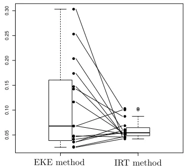
latent trait of a good rainy season) change considerably (see Figure 4(a)). This suggests that the methods are mostly capturing different beliefs of the experts. In addition, the overall uncertainty is lower (Figure 4(b)), suggesting that the IRT method tends to increase the prophets’ self confidence in answering the objective questions, reducing the uncertainty about their prior belief.

As discussed in O’Hagan et al. (2006), the decision maker, typically the researcher interested in the prophets’ opinions, can treat multiple prophets as data; that is, he/she should make his/her own reasoning about the parameter and then update it with the prophets’ prior distributions. Roughly

speaking, given the prophets prior distributions πj(θj) (j = 1, ..., k), we should decide a sensible

(14)

0.2

0.3

0.4

0.5

0.6

0.7

0.8

0.9

EKE method IRT method

(a) Means (the probability and the latent trait of a good rainy season)

0.05

0.10

0.15

0.20

0.25

0.30

EKE method IRT method

[image:14.595.316.499.98.263.2]

(b) Standard deviations

Figure 4.: Comparison of how the prior means and standard deviations change from of the EKE and the IRT methods.

than other, thus it seems natural to consider the global prior distribution as

π(θ) =

k X

j=1

wjπj(θj), (10)

wherewj are weights attributed to each prophet’s opinion. There are many ways to combine prior

densities, reviews can be found in Genest and Zidek (1986) and Clemen and Winkler (1999).

On the other hand, using exclusively the IRT model, we can combine the opinions from the IRT questionnaire by simply considering the model

Yij|θ∼ Ber(P) (i.i.d.)∀i, j,

θ∼ Uniform(0,1), (11)

where P = exp (1/(1−θ)−1/θ) [1 + exp (1/(1−θ)−1/θ)]−1_{. In this way the proportion of}

posi-tive responses will indicate higher values of the latent trait. The global prior variance will be based on the proportion of items which the prophets responded “yes” and those who answered “no”,

since all the items were conceived to indicate high values of θ when the answer is positive and,

otherwise when the answer is “no”, all the answers together represent some uncertainty which will be captured by the variance.

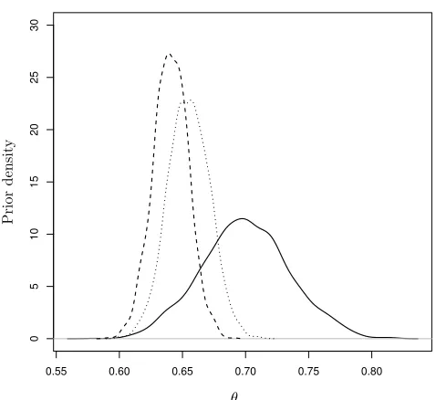
We compare the three resulting prior distributions forθ(Figure 5): the combination (11) obtained

from the EKE method, from the IRT method, that is using (10) to combine the pj(θj) and using

(15)

latent trait.

0.55 0.60 0.65 0.70 0.75 0.80

0

5

10

15

20

25

30

θ

P

ri

or

d

en

si

[image:15.595.180.419.123.342.2]

ty

Figure 5.: Combined prior distributions ofθ: EKE

method (continuous line), IRT methods (dotted line) and IRT method using (11) (dashed line).

4. Concluding remarks

The fundamental idea of using IRT as an EKE tool is to create a questionnaire with simple dichoto-mous questions that are directly associated with the quantity of interest. Thus, instead of trying to make the expert to think about the possible values of the parameter, which is challenging in many settings, the expert is asked to consider which scenarios will or will not happen. The process of creating the questionnaire, as in general EKE protocols, should be rigorous and address issues related to heuristics and biases. Most importantly, both the expert and the facilitator should come together to assess which scenarios are most closely associated with the latent trait. Since the pro-posed method results in a prior distribution that is not from a common conjugate family, we also have the flexibility to more closely match the experts’ beliefs.

As we have shown in the present paper, the procedure is suitable for any number of experts. When many experts are available, we can add the discrimination and the difficulty parameters to the IRT model. In fact, some items might have been inadequately chosen in the sense that a long run experience in a specific setting could show that the item is not suitable to capture the latent trait. This can allow greater insights regarding the items themselves and the efficacy of the items in measuring the latent trait. As we gain more experience of applying this method, prior distributions for the item parameters may be proposed since we may be able to prejudge the effectiveness of the individual questions.

(16)

applied, steps will need to be taken to check how the proposed model fits to related data and the assumptions underpinning the model. In the context of IRT in general, there are several strategies used to assess the model. Fox (2010) provides several methods to check the model fit: in the context of expert’s elicitation, the main procedures listed by Fox (for example, residual analyses and posterior predictive assessment) require a large number of experts. Having a large number of experts involved in elicitation is rare, and smaller sample methods will need to be devised to assess the adequacy of the method. Alongside this, to further understand the implications of the various model assumptions, research is required to determine the impact of not having assumptions of the local and inter-expert independence satisfied, which will become possible as the method is more widely applied.

Acknowledgement:We thank the Associate Editor and the Referees for the comments and sug-gestions which improved considerably the presentation of our work.

References

Albert, J. H. (1992). Bayesian estimation of normal ogive item response curves using Gibbs

sam-pling. Journal of Educational Statistics,17(3), 251–269.

Albert, J. H. (1998). An investigation of the item parameter recovery characteristics of a gibbs

sampling procedure. Applied Psychological Measurement,22(1), 163–169.

Albert, J. H. and Chib, S. (1993). Bayesian analysis of binary and polychotomous response data.

Journal of the American Statistical Association,88(422), 669–679.

Andrade, J. A. A. and Gosling, J. P. (2008). Estat´ıstica busca apontar chances de bom inverno,

Di´ario do Nordeste:

http://diariodonordeste.verdesmares.com.br/cadernos/regional/estatistico-avalia-estudo-dos-profetas-das-chuvas-1.622816.

Andrade, J. A. A. and Gosling, J. P. (2011). Predicting rainy seasons: quantifying the beliefs of

prophets. Journal of Applied Statistics,38, 183–193.

Baker, F. B. (2001). The basics of item response theory. ERIC.

Burgman, M. A. (2015). Trusting Judgements: How to Get the Best out of Experts. Cambridge

University Press.

Clemen, R. T. and Winkler, R. L. (1999). Combining probability distributions from experts in risk

analysis. Risk Analysis,19, 187–203.

Cooke, R. M. (1991). Experts in uncertainty: opinion and subjective probability in science. De Roos, Y. and Allen-Meares, P. (1998). Applications of Rasch analysis: exploring differences in

depression between African-American and white children. Journal of Social Service Research,23

(3–4), 93–107.

Du, C., Kurowicka, D., and Cooke, R. M. (2006). Techniques for generic probabilistic inversion.

Computational Statistics & Data Analysis,50(5), 1164–1187.

Flari, V., Chaudhry, Q., Neslo, R., and Cooke, R. (2011). Expert judgment based multi-criteria de-cision model to address uncertainties in risk assessment of nanotechnology-enabled food products.

Journal of Nanoparticle Research,13(5), 1813–1831.

Fox, G., Berg, S. v. d., and Veldkamp, B. (2015). Bayesian psychometric scaling. In: P. Irwing &

T. Booth & D. Hughes (Eds.), Handbook of psychometric testing.

Fox, J. P. (2010). Bayesian item response modeling: Theory and applications. New York, NY:

Springer.

Fox, J. P. and Glas, C. A. (2001). Bayesian estimation of a multilevel IRT model using Gibbs

sampling. Psychometrika,66(2), 271–288.

Fu, Z., Tao, J., and Shi, N. (2009). Bayesian estimation in the multidimensional three-parameter

(17)

Genest, C. and Zidek, J. V. (1986). Combining probability distributions: a critique and an annotated

bibliography. Statist. Sci.,1, 114–35.

Gosling, J. P., Hart, A., Mouat, D. C., Sabirovic, M., Scanlan, S., and Simmons, A. (2012).

Quanti-fying experts’ uncertainty about the future cost of exotic diseases. Risk Analysis,32(5), 881–893.

Hambleton, R. K., Swaminathan, H., and Rogers, H. J. (1991). Fundamentals of Item Response

Theory. Newbury Park, CA: Sage Press.

Jaspersen, J. G. and Montibeller, G. (2015). Probability elicitation under severe time pressure: A

rank-based method. Risk Analysis,35(7), 1317–1335.

Jungermann, H. and Zeeuw, G. (1977). Decision making and change in human affairs, volume 16.

Springer Science & Business Media.

Kadane, J. B. and Wolfson, L. J. (1998). Experiences in elicitation. The Statistician, pages 3–19.

Kirkwood, C. W. and Sarin, R. K. (1985). Ranking with partial information: A method and an

application. Operations Research,33(1), 38–48.

Kriegler, E., Hall, J. W., Held, H., Dawson, R., and Schellnhuber, H. J. (2009). Imprecise probability

assessment of tipping points in the climate system. Proceedings of the National Academy of

Sciences,106(13), 5041–5046.

Kurowicka, D., Bucura, C., Cooke, R., and Havelaar, A. (2010). Probabilistic inversion in priority

setting of emerging zoonoses. Risk analysis,30(5), 715–723.

Lee, Y. (2004). Examining passage-related local item dependence (LID) and measurement construct

using Q3 statistics in an EFL reading comprehension test. Language Testing,21(1), 74–100.

Matteucci, M., Mignani, S., and Veldkamp, B. P. (2012). Prior distributions for item parameters

in IRT models. Comm. Statist. Theory Methods,41(16–17), 2944–2958.

Morgan, M. G., Morris, S. C., Henrion, M., Amaral, D. A., and Rish, W. R. (1984). Technical

uncertainty in quantitative policy analysisa sulfur air pollution example. Risk Analysis, 4(3),

201–216.

Morgan, M. G. and Henrion, M. (1992). Uncertainty: a guide to dealing with uncertainty in

quan-titative risk and policy analysis. Cambridge University Press.

O’Hagan, A., Buck, C. E., Daneshkhah, A., Eiser, J. E., Garthwaite, P. H., Jenkinson, D., Oakley,

J. E., and Rakow, T. (2006). Uncertain judgements: eliciting expert probabilities. Chichester:

Wiley.

O’Hagan, A. and Oakley, J. E. (2004). Probability is perfect, but we can’t elicit it perfectly.

Reliability Engineering & System Safety,85(1), 239–248.

Rubin, D. B. (1987). Multiple Imputation for Nonresponse in Surveys. New York: John Wiley &

Sons.

Sheng, Y. and Wikle, C. K. (2009). Bayesian IRT models incorporating general and specific abilities.

Behaviormetrika,36(1), 27–48.

Smith, L. H. (1967). Ranking procedures and subjective probability distributions. Management

Science,14(4), 236–249.

Taddei, R. (2005). Of Clouds and Streams, Prophets and Profits: The Political Semiotics of

Cli-mate and Water in the Brazilian Northeast. PhD thesis, Graduate School of Arts and Sciences, Columbia University.

Torre, J. and Hong, Y. (2010). Parameter estimation with small sample size a higher-order IRT

model approach. Applied Psychological Measurement,34(4), 268–285.

Walley, P. (1996). Measures of uncertainty in expert systems. Artificial intelligence,83(1), 1–58.

Wang, W. and Wilson, M. (2005). Exploring local item dependence using a random-effects facet

model. Applied Psychological Measurement,29(4), 296–318.

Weible, C. M. (2008). Expert-based information and policy subsystems: a review and synthesis.

(18)

Appendix A OpenBugs Codes

A.1. Example 3.1

model ;{

for ( j in 1: J ) { for ( i in 1: I ) {

Y [i , j ] ~ dbern ( p [i , j ])

p [i , j ] <- 1/(1+ exp ( - a [ i ]/(1 - theta [ j ])+1/ theta [ j ]+ b [ i ])) }

}

for ( j in 1: J ) {

theta [ j ] ~ dunif (0 ,1) }

for ( i in 1: I ) {

a [ i ] ~ dgamma (3 ,5)

b [ i ] ~ dgamma (2 ,4) # It should be flat }

}

list(I=20, J=10, Y=structure(.Data =c(1,0,0,0,0,NA,0,0,NA,NA,1,0,0,0,0,NA,0,0,NA,NA,1,

0,0,0,0,NA,0,0,NA,NA,1,0,0,0,0,NA,0,0,NA,NA,1,0,0,0,0,NA,0,0,NA,NA,1,1,0,0,0,NA,NA,0,

NA,NA,1,1,0,0,0,NA,NA,0,NA,NA,1,1,0,0,0,NA,NA,0,NA,NA,1,1,0,0,0,NA,NA,0,NA,NA,1,1,0,0

,0,NA,NA,0,NA,NA,1,1,1,0,0,1,1,NA,0,NA,1,1,1,0,0,1,1,NA,0,NA,1,1,1,0,0,1,1,NA,0,NA,1

,1,1,0,0,1,1,NA,0,NA,1,1,1,0,0,1,1,NA,0,NA,1,1,1,1,0,1,1,1,0,0,1,1,1,1,0,1,1,1,0,0,1,

1,1,1,0,1,1,1,0,0,1,1,1,1,0,1,1,1,0,0,1,1,1,1,0,1,1,1,0,0), .Dim=c(20,10)))

A.2. Example 3.2

model ;{

for ( j in 1:16) { for ( i in 1:33 ) {

Y [i , j ] ~ dbern ( p [i , j ])

p [i , j ] <- 1/(1+ exp ( -1/(1 - theta [ j ])+1/ theta [ j ])) }

}

for ( j in 1:16) {

theta [ j ] ~ dunif (0 ,1) \# U n i f o r m prior }

}

list(Y=structure(.Data = c(1., 1., 0., 1., 1., 1., 0., 1., 1., 1., 1., 1., 1., NA, 0., 1., NA, 1., 1., 1., 1., 1., NA, 1., 1., 1., NA, 1., NA, 1., 0., 0., 1., 1., 1.,

1., 1., 1., NA, 1., 1., 1., 1., 1., 1., 1., NA, 1., 1., 0., 1., NA, NA, 1., NA, NA, 1., 1., NA, 1., NA, NA, NA, 1., 1., 1., 1., 1., 1., 1., NA, 1., 1., 1., 1., 1., 1.,

1., 1., 1., 0., 1., 1., 1., 1., NA, 1., 1., 1., 1., 0., 1., NA, NA, NA, 1., 0., 1., 1., NA, 1., NA, NA, 1., NA, 1., 1., 1., NA, NA, NA, NA, NA, 1., 1., NA, NA, NA, NA,

0., NA, NA, NA, NA, NA, NA, NA, NA, NA, 1., NA, NA, NA, NA, NA, NA, NA, NA, NA, NA, NA, NA, 0., 0., 1., 1., 1., 0., NA, 1., NA, 1., NA, NA, 0., 1., NA, 1., 0., 1., 1.,

1., NA, 1., 1., 1., NA, 1., 1., 1., 0., 1., 1., 1., 1., 0., 0., 1., 1., 0., NA, NA, 0., 1., 1., 0., 1., 1., NA, NA, 0., NA, 1., 1., 1., 1., 1., 1., NA, 1., 1., 1., 0.,

1., 1., NA, 1., 0., 0., 1., 1., 0., 1., NA, 0., 0., 0., 1., 0., 1., NA, NA, 0., NA, NA, NA, NA, 0., NA, 1., NA, NA, NA, NA, NA, NA, NA, NA, NA, NA, 1., 1., 1., 1., NA,

1., NA, 1., 1., 1., 1., 1., 1., NA, 1., 1., 1., 1., 1., 1., NA, 1., NA, 1., 1., NA, 0., 1., NA, 1., 1., 1., 1., 1., 1., 1., NA, 1., NA, 1., 1., 1., 0., 1., NA, 1., 0.,

NA, 1., 1., NA, NA, NA, 1., NA, NA, 1., 0., 0., 1., NA, NA, 0., NA, NA, 1., 1., 1., 0., NA, NA, NA, 1., 0., 0., 1., NA, 1., 0., NA, NA, NA, 1., NA, 1., NA, NA, 1., 1.,

1., 0., 1., NA, NA, 1., NA, 1., 0., NA, NA, 1., NA, NA, 0., 1., NA, NA, NA, NA, NA, NA, NA, NA, 1., 1., NA, 1., 1., NA, 0., 1., 1., NA, NA, 1., NA, NA, 0., NA, 1.,

NA, 0., NA, NA, NA, 1., 0., 0., NA, 1., NA, 1., 0., NA, 1., 1., 1., NA, NA, NA, NA, 1., 1., NA, 0., 1., NA, NA, NA, 0., 1., NA, 1., 1., 0., NA, NA, 1., 1., NA, NA,

1., NA, NA, NA, NA, NA, 1., NA, 0., NA, 0., NA, NA, 1., 0., 0., 1., NA, NA, 0., 0., NA, NA, NA, NA, NA, NA, NA, 0., NA, NA, NA, NA, NA, NA, NA, NA, NA, 1., 0., NA,

(19)

1., NA, NA, NA, 1., 1., NA, NA, 1., NA, 1., NA, NA, NA, NA, NA, NA, 0., NA, NA, 1., 1., NA, NA, NA, NA, 1., 1., NA, 0., 1., NA, NA, 0., NA))

Appendix B IRT Questionnaire

(1) Will the small water reservoir in the region will get full? (2) Did the bees suggest a good rainy season?

(3) Will the low lands will be wet throughout the season?

(4) Did the ‘‘caranguejeira’’ spider suggest a good rainy season?

(5) Will the leafs of the plants will turn green? (6) Did the moon suggest a good rainy season?

(7) Did the October sun rising suggest a good rainy season? (8) Did the ‘‘serra-pau’’ beattle a good rainy season?

(9) Did the ‘‘Caatingueira’’ tree suggest a good rainy season?

(10) Did the ants suggest a good rainy season? (11) Will we have a good grain crop?

(12) Did the new year sun rising suggest a good rainy season? (13) We we have a good milk production?

(14) Did the Christmas sun rising suggest a good rainy season? (15) Did the ‘‘Jo~ao-de-Barro’’ bird suggest a good rainy season? (16) Will we have pasture for the cattle?

(17) Will the ground be wet during the season?

(18) Did the ‘‘Juazeiro’’ suggest a good rainy season?

(19) In general, do the birds suggest a good rainy season? (20) Did the frogs suggest a good rainy season?

(21) Did the termites suggest a good rainy season? (22) Did the sun shadow suggest a good rainy season?

(23) Did the winds suggest a good rainy season?

(24) Did the ‘‘mandacaru’’ suggest a good rainy season? (25) Did the fish are ready for reproduction?

(26) Did the clouds move suggest a good rainy season? (27) Did the ‘‘cumaru’’ suggest a good rainy season?

(28) Did the ground warms suggest a good rainy season? (29) Did the ‘‘pau-darco’’ suggest a good rainy season?

(30) Did the ground temperature suggest a good rainy season? (31) Did the Flamboyant tree suggest a good rainy season? (32) Have you seen flying ants?