Reference Dependence and Market Participation

White Rose Research Online URL for this paper:

http://eprints.whiterose.ac.uk/140430/

Version: Accepted Version

Article:

Guasoni, Paolo and Meireles Rodrigues, Andrea Sofia orcid.org/0000-0003-3357-3879

(2019) Reference Dependence and Market Participation. Mathematics of Operations

Research. ISSN 1526-5471

https://doi.org/10.2139/ssrn.3017830

[email protected] https://eprints.whiterose.ac.uk/ Reuse

Items deposited in White Rose Research Online are protected by copyright, with all rights reserved unless indicated otherwise. They may be downloaded and/or printed for private study, or other acts as permitted by national copyright laws. The publisher or other rights holders may allow further reproduction and re-use of the full text version. This is indicated by the licence information on the White Rose Research Online record for the item.

Takedown

If you consider content in White Rose Research Online to be in breach of UK law, please notify us by

PaoloGuasoni† AndreaMeireles-Rodrigues‡

27th November 2018

Abstract

This paper finds optimal portfolios for the reference-dependent preferences by K˝oszegi and Ra-bin, with piecewise linear gain-loss utility, in a one-period model with a safe and a risky asset. If the return of the risky asset is highly dispersed relative to its potential gains, two personal equilib-ria arise, one of them including risky investments, the other one only safe holdings. In the same circumstances, the risky personal equilibrium entails market participation that decreases with loss aversion and gain-loss sensitivity, whereas the preferred personal equilibrium is sensitive to market and preference parameters. Relevant market parameters are not the expected return and standard deviation, but rather the ratio of expected gains to losses and the Gini index of the return.

JEL Classification: G11, G12.

AMS MathematicsSubjectClassification(2010): 91G10, 91G80.

Keywords: loss aversion; market participation; personal equilibria; portfolio choice; reference dependence.

∗_{For helpful comments, we thank Rabah Amir and Tomasz Zastawniak, as well as seminar participants at the University} of Edinburgh, University of Manchester, MTA Alfréd Rényi Institute of Mathematics, Business Research Institute-IUL, and 10th World Congress of the Bachelier Finance Society. We are also grateful to two anonymous referees and associate editor for their thoughtful and constructive suggestions, which substantially improved the paper. Part of this research was carried out while Meireles-Rodrigues was affiliated with the School of Mathematical Sciences, Dublin City University, Ireland. This work was partially supported by the ERC (279582), NSF (DMS-1412529), and SFI (16/IA/4443 and 16/SPP/3347).

†_{Boston University, Department of Mathematics and Statistics, 111 Cummington Mall, Boston, MA 02215, USA, and} Dublin City University, School of Mathematical Sciences, Glasnevin, Dublin 9, D09 W6Y4, Ireland, [email protected]. ‡_{Department of Mathematics, University of York, Heslington, York, YO10 5DD, UK,} [email protected].

1

Introduction

Standard portfolio theory imagines investors as utility maximizers, unencumbered by personal past ref-erences, who are sensitive to consumption and wealth outcomes alone. An important implication is that every such investor should participate, however little, in investments carrying a positive risk premium: using the words ofHuang and Litzenberger(1988), “An individual who is risk averse and who strictly prefers more to less will undertake risky investments if and only if the rate of return on at least one risky asset exceeds the risk-free interest rate.”

In reality, less than half of households participates in the stock market (Guiso, Haliassos, and Jap-pelli,2002;Vissing-Jorgensen,2003), and the prospect theory ofKahneman and Tversky(1979) recog-nizes reference dependence as a major determinant of preferences, though it remains silent on the origin of such references. Filling this void,Shalev(2000) argues that “Reference points emerge as expressions of anticipation which are fulfilled”, andK˝oszegi and Rabin (2006) stipulate that reference points are “rational expectations held in the recent past about outcomes”.

This paper solves the one-period portfolio choice problem for an investor with the reference-de-pendent preferences ofK˝oszegi and Rabin(2006), and finds that its solution supports two competing personal equilibria—expectations about one’s choice that make such choice optimal. One personal equi-librium involves a mix of risky and safe investments, and is a variant of the familiar utility-maximizing portfolio of Markowitz(1952). The additional equilibrium involves only safe investments, and offers an explanation for non-participation in the market based on reference-dependent preferences: for an in-vestor expecting to take risk, it is optimal to do so to the extent specified by the risky equilibrium. Yet, for an investor with the same preferences but with the expectation to hold safe assets, it is optimal to forgo risky assets completely.

The reference-dependent preferences ofK˝oszegi and Rabin(2006) prescribe that the overall value of a payoffresults from its standard expected utility plus a further component that measures the satisfaction or disappointment of the payoffin comparison to another reference payoff. The comparison is performed by averaging a gain-loss function over all possible payoff-reference pairs, each of them weighted by its respective probability. This gain-loss function is “kinked” at the origin, with a steeper slope for losses than for gains to reflectloss aversion—“losses loom larger than gains” (Kahneman and Tversky,1979). While K˝oszegi and Rabin (2006, 2007, 2008, 2009) develop reference-dependent preferences at increasing levels of generality, their implications for portfolio choice have hitherto remained unexplored, and this paper starts to fill this gap. The central difference from previous models of reference dependence (cf. Bernard and Ghossoub,2010;He and Zhou,2011) is that the reference point is endogenous, and therefore needs to be identified as part of the optimization.

Two main issues arise: First, as optimal choices depend on the reference as well as the utility, multiple optimal portfolios may exist, even with a strictly concave utility function. Second, a reference must be a personal equilibrium, in that it needs to be the optimal payofffor those who adopt it as a reference, e.g., investors cannot increase their utilities by adopting unrealistically low references as to surprise themselves with brilliant results. In mathematical terms, a fixed-point problem appears.

We characterize all the personal equilibria in a one-period model of portfolio choice: First, we solve the optimization problem for an arbitrary reference. Then, we identify those references that reproduce themselves as optimal payoffs. Among them, we further determine the preferred personal equilibrium— the ideal reference that an investor unencumbered by a past reference would choose.

We find that the statistical attributes of asset returns that separate the participation and non-partici-pation regimes are not the first two moments typical of mean-variance analysis, but rather the gain-loss ratio and the Gini index. The ratio of expected gains to expected losses varies from zero for a sure loss to infinity for a sure gain, and already appears in the work ofBernardo and Ledoit (2000), who investigate the asset pricing restrictions for the gain-loss ratio, in analogy to the analysis ofHansen and Jagannathan(1991) on Sharpe ratios. Reference-dependent preferences make this ratio prominent as a result of loss-aversion, and offer theoretical support for its use in asset pricing.

reference-dependent utility, which contributes to preferences through the expected gain-loss of payoff-reference outcomes. As payoff and reference are sampled independently in this definition, and our gain-loss function is piecewise linear, it follows that the expected gain-loss of a personal equilibrium is a function of the the mean-absolute difference1of such payoff, and the Gini index coincides with the mean-absolute difference divided by twice the mean.

The Gini index also affects the incidence of market participation and non-participation. As the main result (Theorem 3.4 below) shows, and in contrast to the initial quote from Huang and Litzenberger (1988), a risky asset with high gain-loss ratio (hence expected return) is not sufficient to guarantee par-ticipation, which in turn requires that the return’s Gini index is sufficiently low. Even then, participation and non-participation may coexist as two competing personal equilibria, each of which is optimally chosen by those who already take it as a reference. Of these two personal equilibria, which one is preferred depends on parameter values, as we demonstrate by studying a model in detail.

The paper proceeds as follows: Section2describes the model and formulates the reference-depen-dent optimization problem; Section3states the main results and discusses their significance; Section4 focuses on a model with exponential utility and Gaussian returns, calculating in detail optimal portfolios and their performance; Section5 discusses further implications and concludes. All proofs are in the appendix.

2

Model

Consider a one-period model in which an investor trades at time 0 and evaluates the payoffat timeT, when its return is revealed. The market includes a safe asset with constant interest rater _{≥ −}1, so that the gross return 1+ris non-negative, and a risky asset withexcess returndescribed by a random variable Xdefined on a probability space (Ω_,F_,P_).

At time 0, no information is available (i.e., theσ-algebraF₀ =_{∅_,Ω_{}is trivial), while at timeT all}

information is revealed (i.e.,F_T =F_{). Thus, a self-financing portfolio is described by the initial capital}

w0and the exposureφ∈Rto the risky asset at time 0. Its terminal value is

V_Tφ=w_f0+φX,

wherew_f0≔w0(1+r) denotes the compounded initial wealth.

The next assumption ensures that the utility function is smooth and the usual utility maximization problem is well-posed.

Assumption2.1.

(i) The risky asset return X is integrable (i.e.,E_{[|X|]< +∞), arbitrage-free}2 _(i.e.,P_{{X>0} > 0and} P_{{X<0}>0), and has a bounded density f(·)with respect to the Lebesgue measure on}R_.3

(ii) Theutilityfunction u : R _→ R_{is strictly increasing, concave, and continuously differentiable.} Moreover, there existsǫ >0such that

E_u′_{(α+βX)<+∞ and} Eh_u′_(α+βX)1+ǫ_|X|2+2ǫi_{<+∞ for allα, β∈}R_{. (2.1)}

The above market structure is deliberately simple, as the paper’s main focus is on preferences, which follow the reference-dependent framework ofK˝oszegi and Rabin(2006). The total welfare of a payoffZ results from the usual expected utilityE_{[u(Z)], plus a further contribution that reflects the disappointment} or satisfaction fromZin relation to some stochastic reference payoffB. Such contribution is computed

1 _{Themean-absolute differenceof a random variableXis defined asE[}

|X₋Y_|], whereYis independent ofXand identically distributed.

2 _{The caseX=0 almost surely (a.s.) is trivial and hence excluded here.} 3 _{The boundedness of f(}

·) can be replaced with the weaker, but more cumbersome conditionR_Rf(x)2+1_{ǫ dx<+}

as follows: upon receiving the payoffZ, the agent evaluates the utility surpriseu(Z)₋u(B) according to some gain-loss functionν(_·) that is kinked at the origin to reflect the higher disappointment from a given utility loss than the satisfaction from a utility gain of equal size. The resulting gain-lossν(u(Z)₋u(B)) is then aggregated across all possible values ofZ andB, each pair weighted according to its respective probability.

The above informal description crystallizes into the following definition.

Definition2.2 (Reference-dependent utility(K˝oszegi andRabin,2006)). Thegain-lossfunctionν: R→

R_{is of the form}4

ν(x)≔ν+ x+11[ 0,+_∞)(x)−ν− x−11(−∞,0)(x), for allx∈R,

whereν_±: [ 0,+_∞) _→R_{satisfy the following assumptions:}

(A1) ν_±(_·) are continuous on [ 0,+_∞) , strictly increasing on [ 0,+_∞) , twice-differentiable on (0,+_∞), andν_±(0)=0;

(A2) (Risk aversion on gains and risk propensity on losses)ν_±′′(x)≤0 for allx>0;

(A3) (Loss aversion)ν+(y)−ν+(x)< ν₋(y)−ν₋(x) for allx,y∈(0,+∞) withx<y, and

λ≔ ν

′ +(0)

ν′ −(0) ∈

(0,1), (2.2)

whereν′_±(0) denote the right (+_{) and left (−) derivatives ofν(·) at 0.}

Thereference-dependent utilityof a payoffZwith respect to the referenceBis defined as

U(Z_|B)≔E_[u(Z)]+E

"Z

R

ν(u(Z)₋u(b))dP_B(b)

#

=

Z

R Z

R

[u(z)+ν(u(z)₋u(b))]dP_B(b)dP_{Z(z), (2.3)}

whereP_ZandP_{B are the probability laws ofZandB, respectively.}5

Though K˝oszegi and Rabin (2006) define reference-dependent utility for general S-shaped gain-loss functionsν(_·), which make agents potentially risk-seeking in losses, this paper focuses on a more parsimonious setting, in whichν(_·) is piecewise linear for gains and losses, with a concave kink at zero that preserves loss aversion.

Assumption2.3.For someη∈(0,1),

ν+(x)≔

λη

1₋ηx and ν−(x)≔ η

1₋ηx, for all x∈[ 0,+∞).

4 _Here,x±_{≔max{±x,0}for allx∈}R. In addition, 11A: X→ {0,1}denotes theindicator functionof the setA⊆X, defined

as

11A(x)≔ (

1, ifx_∈A,

0, otherwise.

5 _{Note that the product measureP}

B×PZin (2.3) reflects the evaluation of the gain-loss function, in which each outcome ofZ

is compared to all possible values of the referenceB. Thus, the above expressions could be written in the appealing form

U(Z_|B)=E[u(Z)]+E[ν(u(Z)₋u(B))],

whereZandBare independent random variables. This expression is more compact, but it is also partly misleading, as it suggests that the random variables are compared outcome-by-outcome. While this is technically true in the product space (Ω_×Ω,F_⊗F,P_⊗P_{), it is conspicuously false in the original probability space. In fact, all that is necessary to define (2.3)}

The advantage of this parametrization is to reduce reference-dependence to the two parametersη, λ_∈

(0,1). The parameterλis a measure of loss tolerance (cf.Abdellaoui, Bleichrodt, and Paraschiv,2007), defined as the ratio between sensitivity to gains and sensitivity to losses, as in Benartzi and Thaler (1995); Köbberling and Wakker(2005): λ _↓ 0 represents extreme sensitivity to losses, which makes gains irrelevant, whileλ= 1 recovers the usual case of a smooth utility, with equal sensitivity for gains and losses. The parameterηcontrols the relative weights of classical versus reference-dependent utility in the overall objective, with η = 0 recovering the classical setting, and η _↑ 1 the pure reference-dependent limit. (Elsewhere in the literature, e.g.,Tversky and Kahneman(1992), the symbolλdenotes loss aversion, defined as the ratio between small losses and equal-sized gains, which corresponds to 1/λ

in our notation. This paper prefers to focus on loss tolerance, which is between zero and one, and hence allows to display parameter regimes in the foregoing figures without axis distortions.)

Reference-dependent preferences lead to the two central concepts ofpersonal equilibriumand pre-ferred personal equilibrium. Informally, a personal equilibrium is a payoffthat is optimal when used as reference: if the agent takes such a strategy as a reference, then the strategy is indeed chosen. In this sense, personal equilibria are the only rational references, which are actually selected once adopted.

As personal equilibria can be numerous and each of them may have a different utility, the question arises of which personal equilibrium is optimal, leading to the concept of preferred personal equilib-rium, a personal equilibrium that is not surpassed by any other. A rational forward-looking agent, unencumbered by a legacy reference, necessarily chooses a preferred personal equilibrium.

Definition2.4 (Personal equilibria).

(i) A portfolioφis apersonal equilibriumwith initial wealthw0if

sup ϕ∈R

UV_TϕV_Tφ=U

V_TφV_Tφ

, (2.4)

and PE(w0)⊆Rdenotes theset of personal equilibria.

(ii) A portfolioφ_∈PE(w0) is apreferred personal equilibriumif

v∗(w0)≔ sup

ϕ∈PE(w0)

UV_TϕV_Tϕ=U

V_TφV_Tφ

,

and PPE(w0)⊆Rdenotes theset of preferred personal equilibria.

3

Main Results

3.1 Linear utility

The first result of the paper identifies personal equilibria in the special case of a linear utility function u(_·). In the context of reference-dependence, a linear utility does not imply risk neutrality, in view of loss aversion in the reference-dependent component.

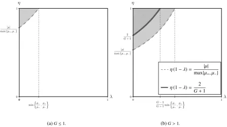
The theorem below finds that three regimes arise: (i) there are no personal equilibria;(ii) the safe portfolio is the unique personal equilibrium; and(iii)any risky position with positive expected return (including zero) is a personal equilibrium. These conclusions are illustrated in Figure1, which displays the parameter combinations in which each regime arises.

Theorem3.1.Let u(·)be linear,µ ≔E[X] , 0, and let Assumptions2.1and2.3 hold. Also, setµ_± ≔ E_X±_{, and denote theGini indexof the distribution of X by}

G≔ 1

|µ_|

Z

R

(i) (Personal equilibria)

(a) If

1₋η(1₋λ)_≤ µ+

µ₋ ≤

1

1₋η(1₋λ) (3.1)

and

1₋η(1₋λ), G−1

G+1 (3.2)

both hold, then PE(w0)={0}, where0is the portfolio with all wealth in the safe asset.

(b) If (3.1)holds but(3.2)fails, then PE(w0)={φ∈R: φµ≥0}.

(c) If (3.1)fails, then PE(w0)=∅.

(ii) (Preferred personal equilibria)

If (3.1)holds, then PPE(w0)={0}. Otherwise, PPE(w0)=∅.

Proof. See AppendixA.2.

Remark3.2. Condition (3.1) is equivalent to the condition

1+ν′ +(0) 1+ν′

−(0) ≤

µ+

µ₋ ≤

1+ν′ −(0) 1+ν′

+(0)

(3.3)

identified inK˝oszegi and Rabin(2007, Proposition 11(i)) as necessary for a zero lottery to be a personal equilibrium, and sufficient for it to be preferred tosufficiently smallfavorable bets (with a safe reference). By contrast, Theorem3.1implies, under the same condition, that the safe investment combined with the safe reference is strictly better thanallrisky portfolios combined with the safe reference, hence (3.3) is also sufficient for the existence of the safe personal equilibrium. Note also that the potentially unbounded random variables considered here raise the integrability issues addressed in LemmaA.3below.

(a)G_≤1.

η(1₋λ)= |µ| max{µ+, µ_−}

η(1₋λ)= 2

G+1

(b)G>1.

Figure 1:The set of personal equilibria of an investor with linear utility (in a market whereµ,0) is defined by

the relation between the investor’s loss toleranceλon the x-axis and reference-dependenceηon the y-axis. The

three regions represent the sets of personal equilibria for all combinations of the parametersλandη: PE(w0)=∅

Even a cursory look at this result immediately highlights some stark differences from usual portfolio theory. First, an asset’s appeal is measured not by its expected return, but rather by itsgain-loss ratio

µ+/µ₋. Bernardo and Ledoit(2000) postulated such ratio as the central element of their asset pricing model: here it arises from the combination of loss-aversion with reference-dependent utility. Second, the risk of an asset is not described by variance, but rather by the Gini indexG, a measure of disper-sion introduced byGini(1912) and commonly used in the inequality literature, but apparently novel in portfolio choice. Note, however, that while the Gini index of a distribution with positive support varies between 0 (no dispersion) and 1 (extreme dispersion), the Gini index of a random variable taking pos-itive as well as negative values, such as the excess return considered here, can take values above one (LemmaA.7below offers bounds for the Gini index in terms of the Sharpe ratio).

The main message of Theorem 3.1 is that, if expected gains are not significantly different from expected losses, as captured by thegain-loss ratioµ+/µ₋, then the only risk-neutral preferred personal equilibrium is the fully safe portfolio. That the safe portfolio is a personal equilibrium is not surprising in view of loss aversion, which creates a tension between positive expected returns, emphasized by classical utility, and expected losses, emphasized by the reference-dependent component. The deeper question is whether other personal equilibria exist.

Condition (3.2) characterizes the uniqueness of the safe personal equilibrium, which holds unless the Gini coefficient of the risky asset has the critical value for which (3.2) fails (i.e., equality holds). Such a result appears puzzling at first, as the safe asset is the unique personal equilibrium for values of 1₋η(1₋λ) both below and above, but not equal to (_|G_{| −}1)/(_|G_|+1). Behind such apparent singularity lie two sharply different reasons for a unique equilibrium below and above 1₋η(1₋λ). Below such threshold, loss aversion is strong enough to make an investor wish for a safer portfolio, no matter what the reference payoff: the safe personal equilibrium is “stable”.

Above the threshold, the opposite occurs: loss aversion is so weak that any risky reference payoff

encourages even more risk (and return), whence equilibrium fails unless the reference portfolio is safe, which represents an “unstable” equilibrium. At the threshold, loss aversion encourages neither more nor less risk taking, making any strategy with positive expected return a personal equilibrium. This interpretation is further supported by Theorem3.4below in the context of risk aversion, which leads to multiple equilibria. Note also that6

G₋1 G+1 =−

E_[X∧Y]

E_[X∨Y], (3.4)

where the random variableY is independent of, and identically distributed to the excess return. Thus, the right-hand side of (3.4) can be interpreted as the opposite of a min-max ratio, a scale-invariant attribute that describes how far the average minimum of two independent outcomes is from the average maximum.7

In summary, reference dependence induces a delicate tradeoffbetween loss aversion and gain-loss ratios even for linear utilities, generating two main regimes: either the safe asset is the only preferred per-sonal equilibrium, or no equilibrium exists. The preferred safe equilibrium region contains a borderline case with infinitely many equilibria.

Remark 3.3 (Long Positions Constraint). The non-existence of personal equilibria in Theorem 3.1 stems from the absence of constraints on risky positions, which lead a risk-neutral utility maximizer to take arbitrarily large risks when they are sufficiently attractive. (Put differently, neither the set of trading strategies nor the superlevel sets of the objective are compact—unlike Theorem 3.4 below.8) Alternative assumptions of interest include the possibility that neither leverage nor short sales are al-lowed, whence the strategy must lie in the interval [0,w0], and a personal equilibrium always exists. An

inspection of the proof in the appendix reveals that, under such constraint, the statement of Theorem3.1

6 _Here,x

∨y≔max_{x,y_}andx_∧y≔min_{x,y_}, for allx,y_∈R_. 7 _{Note also that the min-max ratio is strictly between}

−1 and 1, and that the Gini index and min-max ratio of a (purely atomic) Dirac lawδx₀, for somex0∈R\ {0}, are equal to 0 and 1, respectively.

8 _{In this respect, our setting differs from the standard environment ofK˝oszegi and Rabin(2006), in which the action set is}

changes as follows:

(i’) (Personal equilibria)

(a’) If, in addition to (3.1),

1₋η(1₋λ)> G−1

G+1, (3.5)

then PE(w0)={0,w0}.

(b’) If, in addition to (3.1),

1₋η(1₋λ)< G−1

G+1, then PE(w0)={0}.

(c’) If (3.1) holds but (3.2) fails, then PE(w0)=[0,w0].

(d’) If (3.1) fails, then PE(w0)={w0}.

(ii’) (Preferred personal equilibria)

If (3.1) holds, then PPE(w0)={0}. Otherwise, PPE(w0)={w0}.

3.2 Concave utility

With concave utilities, risk aversion arises from both the utility function and the loss aversion in the reference-dependent component. The next result characterizes the optimal solution in this setting, in which a personal equilibrium always exists. In fact, two personal equilibria typically compete for op-timality: one is the safe asset, as for linear utility. The other one involves a mix of safe and risky investments, and converges to the usual maximizer of expected utility as reference-dependence van-ishes.

Theorem3.4.Let u′(·)be strictly decreasing with u′(−∞)= +∞,µ,0, and let Assumptions2.1and2.3 hold.

(i) (Personal equilibria)

(a) If

1₋η(1₋λ)_≤ µ+

µ₋ ≤

1

1₋η(1₋λ) (3.1)

and

1₋η(1₋λ)> G−1

G+1 (3.5)

both hold, then PE(w0)={0, θ∗}for someθ∗≡θ∗(η, λ)such thatθ∗µ >0.

(b) If (3.1)holds but(3.5)fails, then PE(w0)={0}.

(c) If (3.1)fails, then PE(w0)={θ∗}.

(ii) (Preferred personal equilibria)

If (3.1)holds and G_≥1, then PPE(w0)={0}. If (3.1)fails, then PPE(w0)={θ∗}.

Proof. See AppendixA.2.

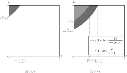
(a)G_≤1.

η(1₋λ)= |µ| max{µ+, µ_−}

η(1−λ)= 2

G+1

(b)G>1.

Figure 2:Regions of different sets of personal equilibria in the parameter space(λ, η)for an investor with strictly

concave utility and unbounded marginal (in a market whereµ,0): PE(w0)={θ∗}on , PE(w0)={0, θ∗}on

, and PE(w0)= {0}on . The dashed curve and the dotted curve represent the existence boundary of the

safe personal equilibrium and of the risky personal equilibrium, respectively.

Figure2displays the regimes arising for different combinations ofηandλ. Weak loss aversion (λ

near one) or reference-dependence (η near zero) generate a single personal equilibrium that includes both safe and risky investments, as in the usual expected-utility setting. In this regime, the asymmetry between gains and losses is not sufficient to alter the qualitative structure of the solution.

As reference dependence and loss aversion increase, the safe equilibrium emerges, coexisting with the classical one (darker region in Figure 2). In such a regime, either equilibrium can be preferred, depending on their respective values, which in turn depend on the specific utility function. If the return of the risky asset is relatively concentrated (G_≤ 1), no other regime is possible. However, if dispersion is high (G > 1), then a third regime arises, in which the safe investment survives as the only, hence preferred, personal equilibrium.

Remark3.6 (LongPositionsConstraint). If leverage and short sales are excluded, the conclusions of Theorem3.4remain valid if the initial capital is sufficiently large andP_{{X<−1−r} > 0. By contrast,} the borrowing constraint is binding whenever the initial capital is small, whence PE(w0) = PPE(w0) =

{0_}if (3.1) holds, and PE(w0)=PPE(w0)=∅otherwise.

The last theorem of this subsection describes the sensitivity of the only risky equilibrium (when it exists) in Theorem3.4to model parameters, such as gain-loss sensitivity, loss tolerance, initial capital, and risk aversion.

Theorem3.7.Let u′(·)be strictly decreasing with u′(−∞)= +∞,µ,0, and let Assumptions2.1and2.3 as well as condition(3.5)hold. Also, denote byθthe unique solution of the classical utility maximization problem, i.e.,

sup ϕ∈R

Eh_uVϕ T

i

=Eh_uVθ T

i

, (3.6)

(i) (Sensitivity to preference parameters)

(a) (Continuity)The mapping(η, λ)7→θ∗(η, λ)is continuous.

(b) (Reference dependence induces less risk taking)For allη, λsatisfying(3.5),

θ∗(η, λ)<_|θ_|. (3.7)

(c) (Monotonicity)The mappingλ 7→θ∗(η, λ)is strictly increasing for anyη∈ (0,1), andη 7→

θ∗(η, λ)is strictly decreasing for anyλ_∈(0,1).

(d) (Classical utility limits)For anyη, λ∈(0,1),lim_λ→1θ∗(η, λ)=θandlim_η→0θ∗(η, λ)=θ. (e) (Pure reference-dependent limits)If G>1, then for allη,¯ λ¯ ∈(0,1)for which(3.2)fails,

lim

(η,λ)→( ¯η,λ¯)θ

∗_{(η, λ)=0.}

If G=1, then

lim

(η,λ)→(1,0)θ

∗_{(η, λ)=0.}

If G<1, then there existsθ¯withθµ >¯ 0and_|θ¯_|<_|θ∗_|such that

lim

(η,λ)→(1,0)θ

∗_{(η, λ)=θ.}¯

(ii) (Sensitivity to risk aversion)

Letη, λ _∈ (0,1) satisfy(3.5), and let ui(·), i ∈ {1,2}, be two utility functions such that u′_i(·) is strictly decreasing with u′_i(_−∞)= +_∞. If u2(·)is aconcave monotone transformationof u1(·), i.e.,

there exists a strictly increasing, concave and differentiable functionρ(_·)such that

u2(x)=ρ(u1(x)) for all x∈R, (3.8)

thenθ∗

1 ≥ θ∗2, whereθ∗i denotes the unique risky personal equilibrium for the reference-depen-dent problem(2.4)with utility ui(·).

(iii) (Sensitivity to initial capital)

Letη, λ_∈(0,1)satisfy(3.5), and assume further that u(_·)is twice-differentiable. Also, denote the Arrow-Pratt coefficient of absolute risk aversion(Arrow,1965;Pratt,1964) of u(_·)by

ARAu(x)≔− u′′(x)

u′_(x), for all x∈R.

If ARAu(·) is non-increasing (respectively, constant or non-decreasing), then∂θ∗/∂w0 is

non-negative (respectively, zero or non-positive).

Proof. See AppendixA.2.

Property(i)(a)states the continuity of the personal equilibrium with respect to the preference para-meters, meaning that slight changes in preference parameters produce only slight changes in the risky personal equilibrium. Equation (3.7) shows that the personal equilibrium implies a lower investment in the risky asset, in view of loss aversion. The interpretation of (i)(c) is that more loss tolerance leads to a riskier position; likewise, the larger the gain-loss sensitivity, the smaller the risky position. Property (i)(d)stipulates that, as the gain-loss sensitivity vanishes either throughηor λ, the personal equilibrium boils down to the unique utility-maximizing portfolio.

G>1, however, then it is not possible for the pair (η, λ) to even approach (0,1), since it can only reach as high as the threshold for existence of the risky personal equilibrium).

A more surprising phenomenon occurs for more concentrated distributions (G<1): then the unique personal equilibrium converges to a nontrivial, nonzero limit, even for an agent solely focused on loss aversion, and insensitive to gains (η_↑1,λ_↓0). At first glance, such a result is puzzling, as the investor has nothing to gain from risk taking. The key here is that an ambitious reference payoffcan induce risky investments, even if gains are disregarded, purely to keep up with the reference by avoiding losses. Put differently, for an investor with a high reference payoff and a moderately concentrated return, opting for the safe asset is an unpalatable choice, as it entails larger losses from the reference than a risky investment that on average comes closer to such target. Thus, such an investor is trapped by a high reference in a non-preferred personal equilibrium, which is inferior to a safe investmentcombinedwith the safe reference.

Turning to (ii), first recall that, if the utilitiesu1(·) andu2(·) are both twice-differentiable then, by

Arrow-Pratt’s theorem (Arrow,1965;Pratt,1964), condition (3.8) is equivalent to replacingu1(·) with

someu2(·) with higher risk aversion thanu1(·). Hence, as for expected utility, higher risk aversion leads

to safer investments.

Finally, property(iii)recovers the same wealth effects for reference-dependent utility as for classical utility: if an agent has constant absolute risk aversion, then the risky personal equilibrium is independent of the initial capital; if an agent’s absolute risk aversion is decreasing (respectively, increasing) in wealth, then the stock is a normal good (respectively, an inferior good)—i.e., the optimal amount allocated to the risky asset increases (respectively, decreases) with the initial capital.

Remark3.8 (RecoveringRiskNeutrality). It is tempting to view Theorem3.1as the limit case of The-orem3.4 as risk aversion vanishes to risk neutrality, but there are perils in such an interpretation. As intuition suggests, in the model in the next section the risky personal equilibrium becomes arbitrarily large as the utility function becomes linear (Proposition4.2(iv))—the risky personal equilibrium disap-pears. Yet, contrary to intuition, it is possible to construct sequences of concave utilities that converge pointwise to a linear function, while the corresponding risky personal equilibria remain confined in a bounded interval (LemmaA.6below). In summary, while risk aversion can be zero only in one way, it can vanish in many ways, and personal equilibria may diverge, converge, or oscillate.

3.3 Ramifications and extensions.

3.3.1 More general gain-loss functions.

Piecewise-linear gain-loss functions conveniently confine the effect of reference-dependence to the loss aversion at the reference point. The question is to what extent the results in the previous section carry over to more general gain-loss functions.

Throughout this subsection, assume thatu(_·) is twice-differentiable, and suppose that Assumption2.3 is replaced by the weaker:

Assumption3.9.For all x,y∈Rsuch that x<y,

−u′′(x)1+ν₋′(u(y)₋u(x))_{≥ −}u′(x)2ν′′₋(u(y)₋u(x)). (3.9)

Lemma3.10.Letµ,0, and let Assumptions2.1and3.9hold.

(i) (Linear utility)

Let u(_·)be linear. Also, setν′_±(+_∞)≔limx→+_∞ν′_±(x)∈[ 0,+∞) and

λ_∞≔ ν

′ +(+∞)

ν′₋(+_∞).

(a) If

G₋1 G+1 ∈ 1−

ν₋(0) (1₋λ_∞) 1+ν₋(0) ,1−

ν₋(0) (1₋λ) 1+ν₋(0)

!

, (3.10)

then PE(w0)\ {0}is non-empty and bounded, and all risky personal equilibria have the same sign

asµ.

(b) If

G₋1 G+1 <

"

1₋ ν−(0) (1−λ∞) 1+ν₋(0) ,1−

ν₋(0) (1₋λ) 1+ν₋(0)

#

, (3.11)

then PE(w0)\ {0}=∅.

(ii) (Concave utility)

Let u′(_·)be strictly decreasing with u′(_−∞)= +_∞. If

1₋ ν ′

−(0) (1−λ) 1+ν′

−(0)

> G−1

G+1, (3.12)

then PE(w0)\ {0}is non-empty and bounded, and all risky personal equilibria have the same sign

asµ.

Proof. See AppendixA.2.

The main difference of this result from the piecewise-linear case is that the number of risky personal equilibria is not determined a priori. For an investor with linear utility, first note thatu(_·) can override risk-propensity on losses only ifν₋(_·) is linear. As conditions (3.10) and (3.11) show, the existence of risky personal equilibria is now also dependent on the new parameterλ_∞; as inHe and Zhou(2011), we denote it as thelarge-loss tolerance(i.e., the analogue of the loss tolerance parameterλ, but for large rather than small payoffs). While part(i)(a)states that there is at least one risky personal equilibrium if (3.10) holds, part(i)(b)is a partial converse result, which makes condition (3.11) essentially sharp, as it leaves open only the borderline case

G₋1 G+1 ∈

(

1₋ ν−(0) (1−λ∞) 1+ν₋(0) ,1−

ν₋(0) (1₋λ) 1+ν₋(0)

)

which needs to be examined model by model, with the exception of ν+(·) linear (which falls in the case(i)(b)of Theorem3.1).

Turning to a strictly concave utility with unbounded marginal, it is still possible to establish the existence of a risky personal equilibrium with positive expected return under condition (3.12), which is a generalization of (3.5). While uniqueness is no longer guaranteed, for all risky personal equilibria the amount of wealth invested in the stock never exceeds a certain level.

3.3.2 Mixed strategies.

of whether randomization can improve an investor’s prospects by increasing the reference-dependent contribution. It turns out that it cannot.

To define mixed strategies, consider the product probability space (Ω_×Ω′_,F _⊗F′_,P_⊗P′_{), where} (Ω_,F_,P_{) is the original probability space describing the uncertainty in the market, while the extrinsic} randomness in the investors’ strategies is modeled by some random variableζ defined on the second probability space (Ω′_,F′_,P′_{). Let}F′

0 be the sigma-algebra generated byζ. Amixed strategystarting

from initial capitalw0is anyF₀′-measurable, integrable random variableψwith terminal value equal to

V_Tψ =w_f0+ψX,

and denote the set of such mixed (or randomized) strategies byR_{. The reference-dependent utility is}

defined by (2.3), the difference being that the integrals are now on the product spaceΩ_×Ω′_{with respect}

to the product measureP_⊗P′_.

Intuitively, it is not worth enlarging the set of strategies to include mixed ones, as these only add more noise to the investors’ payoffwithout improving welfare; this intuition is confirmed by the following lemma. Roughly speaking, part (i)states that an agent planning to adopt a mixed strategy is actually strictly better offchoosing the associated mean (pure) strategy, thus precluding mixed-strategy personal equilibria; by part(ii), for an investor with a pure-strategy reference, taking a mixed strategy never leads to more satisfaction, hence the set of (pure) personal equilibria is not affected by this relaxation of the set of strategies.

Lemma3.11.Let Assumptions2.1 and3.9 hold, and assume that either u(·)is linear or u′(·) is strictly decreasing with u′(_−∞)= +_∞. Then:

(i) For allψ_∈R_\R_,

U

V_TψV_Tψ

<U

V_Tψ¯V_Tψ

,

whereψ¯ ≔E_ψ∈R_.

(ii) For allφ_∈R_,

sup ϕ∈R

UV_TϕV_Tφ= sup ψ∈R

U

V_TψV_Tφ

. (3.13)

Proof. See AppendixA.2.

4

Example

This section examines in detail a concrete model, focusing on exponential utility combined with nor-mally distributed returns.

Assumption4.1.The stock’s excess return X has normal distribution with meanµ∈R\ {0}and standard deviationσ >0. Investors have exponential utility with constant absolute risk aversion coefficientγ >0,

u(x)≔ 1−e −γx

γ , for all x∈R.

In the absence of reference dependence, in this setting the optimal portfolio prescribes an amount invested in the risky asset given by the usual Merton formula:

θM ≔

µ γσ2.

Proposition4.2.Let Assumptions2.3and4.1 hold. Denote by S ≔ _σµ the stock’sSharpe ratio, and by

Φ(_·)the standard normal distribution function.

(i) (a) (Personal equilibria) If

1₋η(1₋λ)_≤ 1+S

√

2πeS 2 2 Φ(S)

1₋S√2πeS22 Φ(S)

≤ ₁ 1

−η(1₋λ) (4.1)

and

1₋η(1₋λ)> 1−

√

π_|S_|

1+ √π_|S_| (4.2)

both hold, then PE(w0) = {0, θ∗}, whereθ∗is the unique solution of the transcendental equation

in z:

µ₋γσ2z 1₋η(1₋λ)+η(1₋λ)Φ γσ_√|z|

2 !!

=η(1₋λ)e−(γσ2z)

2sgn(z)σ

2√π .

If (4.1)holds but(4.2)fails, then PE(w0)={0}. If (4.1)fails, then PE(w0)={θ∗}.

(b) (Preferred personal equilibria)

If (4.2)holds and_|S_{| ≤}π−12, then PPE(w₀)={0}. If (4.2)fails, then PPE(w₀)={θ∗}.

(ii) θ∗_{is strictly increasing inλ,µ; strictly decreasing inη; constant in w0. Moreover,limη}

→0θ∗=θM andlimλ→1θ∗=θM.

(iii) If_|S_|< π−12, thenlim

(η,λ)→(η,¯λ¯)θ∗(η, λ)=0for allη,¯ λ¯ such that

1₋η¯1₋λ¯= 1−

√_π |S_| 1+ √π_|S_|.

If_|S_|=π−12, thenlim_{(η,λ)→(1,0)}θ∗(η, λ)=0. If|S|> π− 1

2, thenlim_{(η,λ)→(1,0)}θ∗(η, λ)=θ¯, whereθ¯is the unique solution of the transcendental equation in z:

µ₋γσ2zΦ γσ_√z

2 !

= σ

2√πe

−(γσz 2 )

2

.

(iv) _|θ∗_|is strictly decreasing inσ,γ; and_|θ∗_|<_|θM|. Moreover,limγ→0|θ∗|= +∞andlimγ→+_∞θ∗=0.

Proof. See AppendixA.2.

The Gaussian distribution has the particularity that its Gini index is inversely proportional to the Sharpe ratio. Consequently, we can write the gain-loss ratio and the opposite of the min-max ratio as, respectively, increasing and decreasing functions of the Sharpe ratio (see (4.1) and (4.2)). As highlighted in the previous section, both of these competing analogues of the Sharpe ratio have significance, in that they give rise to different personal equilibria.

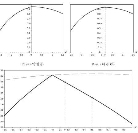
For a suitable choice of market and preference parameters, Figure3shows the graphs of some of the functions associated with the reference-dependent optimization problem. The risk-free rate is fixed at r =1%; the market risk premium and volatility are set equal to 6% and 20% per year, respectively. We select the loss tolerance parameterλ = 0.40 to be consistent with the value estimated byTversky and Kahneman(1991,1992), and the gain-loss sensitivity parameterη = 0.90 so that (4.2) holds and two personal equilibria arise. Finally, the initial capitalw0is normalized to 1, while absolute risk aversion is

0

−1 1

−1.5 −0.5 0.5 1.5

0 1

0.2 0.4 0.6 0.8

0.1 0.3 0.5 0.7 0.9

(a)ϕ_7→UV_TϕV0 T

.

−1.5 −1 −0.5 0 0.5 1 1.5

0 1

0.2 0.4 0.6 0.8

0.1 0.3 0.5 0.7 0.9

(b)ϕ_7→UV_TϕVθ∗ T

.

−0.6 −0.5 −0.4 −0.3 −0.2 −0.1 −0 0.1 0.2 0.3 0.4 0.5 0.6 0.7 0.8 0.9

0.9

0.86 0.88 0.92 0.94 0.96

0.87 0.89 0.91 0.93 0.95

(c)ϕ_7→UV_TϕV_Tϕ(solid line) andϕ_7→EhuV_Tϕi(dashed line).

Figure 3: Plots for an investor with exponential utility when the stock has normal excess return. Market and

preference parameters are: w0 =1, r=1%,γ=3,µ=6%,σ=20%,λ=0.40, andη=0.90; thus, G≈1.88,

0 0.1 0.2 0.3 0.4 0.5 0.6 0.7 0.8 0.9 1 0

1

0.2 0.4 0.6 0.8

0.1 0.3 0.5 0.7 0.9

0.596 0.736

0.877 1.02

1.16

1.3

1.44

1.58

1.72

1.86

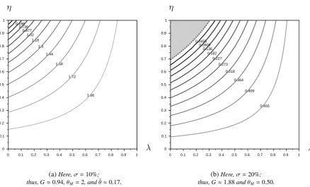
(a)Here,σ=10%; thus, G_≈0.94,θM=2, andθ¯_≈0.17.

0 0.1 0.2 0.3 0.4 0.5 0.6 0.7 0.8 0.9 1 0

1

0.2 0.4 0.6 0.8

0.1 0.3 0.5 0.7 0.9

0.0455 0.0909

0.136 0.182

0.227

0.273

0.318

0.364

0.409

0.455

(b)Here,σ=20%; thus, G_≈1.88andθM=0.50.

Figure 4:Level curves of the mapping(η, λ)7→θ∗_{(η, λ)for an investor with exponential utility when the stock has}

normal excess return. Market and preference parameters are: w0 =1, r=1%,γ=3, andµ=6%.

5

Conclusion

This paper solves the one-period portfolio selection problem underK˝oszegi and Rabin reference-depen-dent preferences. Any risk-averse investor with sufficiently high reference-dependence and loss aver-sion has two competing personal equilibria—strategies that are optimal when taken as references—as individuals with identical preferences may make different investments depending on their expectations. Investors planning to participate in the stock market optimally choose to do so, while those planning to refrain from risky investments optimally hold the safe asset only. The model offers an explanation for limited stock market participation as a result of heterogeneity in references, even in the absence of participation costs.

Although reference-dependent preferences already pose substantial challenges in the one-period set-ting considered here, some of them stem from market incompleteness, which restricts the choice of both references and payoffs. Models of complete markets in both discrete and continuous time offer another setting with significant potential for tractability.

A

Appendix

This appendix contains the proofs of the results stated in the main body of the paper. In what follows,Y is a random variable independent of, and identically distributed toXunderP_.

A.1 Auxiliary results

LemmaA.1.Let Assumption2.1hold. Let b∈R\ {0}, and g: R2 →[ 0,+∞) be a continuous function, differentiable on D≔n(x,y)_∈R2 _{: y−x>0}o_{. If the following conditions hold:}

(i) E_{g(bX,zY)<+∞for all z∈}R_;

(ii) g(x,y)=0for all(x,y)_∈R2_\D;

(iii) x_7→g(x,y)is non-increasing for all y_∈R_;

(iv) for all z_∈R_{, there existsψ}z

1: R→[ 0,+∞) such thatE

h

ψz₁(Y)_|Y_|i<+_∞and

g(bx,(z+h)y)₋g(bx,zy) h

11{(z+h)y−bx>0}≤ψz1(y)|y| for all (x,y)∈R

2_and0<

|h_|<1; (A.1)

(v) for all z_∈R_{, there existsψ}z

2: R→[ 0,+∞) such thatE

h

ψz₂(Y)1+ǫ_|Y_|2+2ǫi<+_∞and

g(zy_{− |}y_|,zy)_≤ψz₂(y)_|y_| for all y_∈R_;

then the functionΓ _: R_→R_{defined by}

Γ_(z)≡Γ_(b;z)≔E_{g(bX,zY) 11}

{zY−bX>0}, for all z∈R, is differentiable onR_{\ {0}, with}

Γ′_(z)=E

"

∂g

∂y(bX,zY)Y11{zY−bX>0} #

, for all z_∈R_{\ {0}.}

Proof. Letb < 0 be given (the proof in the case b > 0 is analogous). Note thatΓ_{(·) is well-defined}

by virtue of(i). Fix an arbitraryz _∈ R_{\ {0}, and consider a sequence{hn}n}

∈Nof nonzero real numbers

converging to 0. Assume further, without loss of generality, that_|hn| < 1 for alln ∈ N. The difference quotient ofΓ_{(·) atzwith incrementhnis equal to}

Γ_(z+hn)−Γ_(z)

hn

=E

"

g(bX,(z+hn)Y)−g(bX,zY) hn

11_{(z+hn)Y−bX>0} #

+E

"

g(bX,zY)11{(z+hn)Y−bX>0}−11{zY−bX>0} hn

#

for alln_∈N_{. We carry out the rest of the proof in two steps.}

(i) We show that limn→+_∞E[Zn]=E

h_∂g

∂y(bX,zY)Y11{zY−bX>0}

i , where

Zn≔

g(bX,(z+hn)Y)−g(bX,zY) hn

11_{(z+hn)Y−bX>0} for alln∈N.

Let ω outside of the null event Ω₁ ≔ _{|X_|= +_{∞} ∪ {|}Y_|= +_{∞} ∪ {}zY =bX_{} ∪ {}Y =0_}, and let ε′(ω) > 0. If zY(ω) ₋ bX(ω) < 0, then (z+hn)Y(ω)− bX(ω) < 0 for all n sufficiently large, so limn→+_∞Zn(ω) = 0 = ∂_∂g_y(bX(ω),zY(ω))Y(ω) 11{zY−bX>0_}(ω). If, on the other hand,

(bX(ω),zY(ω))_∈D, there existsδ >0 such that

g(bX(ω),zY(ω)+h)₋g(bX(ω),zY(ω))

h −

∂g

∂y (bX(ω),zY(ω))

< ε′(ω)

for allh_∈R_{with 0<|h|< δ. Therefore, relabelingε}′_{(ω) asε/Y(ω),}

Zn(ω)−

∂g

∂y(bX(ω),zY(ω))Y(ω) 11{zY−bX>0}(ω)

=g(bX(ω),(z+hn)Y(ω))−g(bX(ω),zY(ω))

hnY(ω) −

∂g

∂y(bX(ω),zY(ω))

|Y(ω)|< ε,

since_|hn|< _|Y(δ_ω)| and (z+hn)Y(ω)−bX(ω)>0 for allnlarge enough. Furthermore, it is an imme-diate consequence of (A.1) that the sequence_{Zn}n∈Nis dominated a.s. by the integrable random

(ii) We claim that

lim n→+_∞

E

"

g(bX,zY)11{(z+hn)Y−bX>0}−11{zY−bX>0} hn

#

=0. (A.2)

To see this, we start by noticing that

E

"

g(bX,zY)11{(z+hn)Y−bX>0}−11{zY−bX>0} hn

#

=

Z

R

f(y)sgn(hny) hn

Z

Iny

g(bx,zy) f(x) dx !

dy, (A.3)

where sgn(_·) is the signum function,9 and Iny is the interval of all real numbers between zy/b and (z+hn)y/b. By Lebesgue’s differentiation theorem, almost every real number belongs to the setL_{f of Lebesgue points of f,}10 _{which in turn implies that Nz} ≔ nby_z : y<L_fo_{has Lebesgue}

measure zero. Next, fix an arbitrary ε > 0, and let y outside of Nz ∪ {0}. It follows from the continuity ofg(_·,_·) that there existsδ1>0 such that

g(bx,zy)=g(bx,zy)₋g(zy,zy)< 1

2

for allx_∈R_{with|x−zy/b|< δ. Moreover, sincezy/b∈}L_{f, there existsδ2 >0 such that}

1 2h

Z

(zy b−h,

zy b+h)

f(x)− f

_zy

b

_{dy< ε}

for all 0<h< δ2. Consequently, for allnsufficiently large,

1

|hny/b|

Z

Iny

g(bx,zy) f(x) dx_≤ 2 2_|hny/b|

Z zy b− hny b ,zy_b+hny_b

g(bx,zy) f(x) dx< ε,

so the sequence of integrands of the outer integral on the right-hand side of (A.3) converges to 0 almost everywhere (asn_→+_∞). Finally, for alln_∈N_{and ally∈}R_,

f(y) 1

|hn|

Z

Iny

g(bx,zy)f(x) dx_≤ 2

|b_|f(y)|y|g(zy− |y|,zy) f ∗zy

b

≤ 2 |b_|f(y)|y|

2_ψz

2(y) f∗

_zy

b

,

where f∗(_·) denotes the maximal function of f(_·).11 _{Moreover, there isC}

ǫ >0 such that Z

R

f(y)_|y_|2ψz₂(y)f∗

_zy b dy ≤ Z R

ψz₂(y)1+ǫ_|y_|2(1+ǫ) f(y) dy ! 1

1+ǫ

Cǫ b z ǫ 2ǫ+1 Z

R

f(y)2ǫǫ+1 _dy ! ǫ

1+ǫ

<+_∞,

by Hölder’s inequality together with the Hardy-Littlewood maximal inequality. Hence, (A.2)

follows from the dominated convergence theorem.

9 _{Thesignum functionsgn : R}

→ {−1,0,1_}is defined by

sgn(x)≔   

−1, ifx<0,

0, ifx=0,

1, ifx>0.

10 _{Recall thatx}

∈R_{is aLebesgue pointof a locally Lebesgue integrable functionf:} R_→R_if

lim

h→0+ 1 2h

Z

(x₋h,x+h)|

f(y)₋f(x)_|dy=0.

11 _{Recall that, given a locally Lebesgue integrable function f : R}

→ R_{, itsHardy-Littlewood maximal function f}∗ _: R_→

[_−∞,+_∞] is defined by

f∗(x)≔sup

r>0

1 2r

Z

(x₋r,x+r)|

The next lemma is, despite its mathematical simplicity, central to our study of personal equilibria. Parts (i) and (ii) imply that investors cannot achieve infinite bliss or grief from any combination of investment strategy and reference payoff. In(iii)and(iv), we study some of the main properties (such as continuity and differentiability) of the reference-dependent utility function given the safe reference and a risky reference, respectively; these are needed, in particular, for obtaining the first-order conditions of LemmaA.3. Lastly, part(v)is used to determine the preferred personal equilibrium.

LemmaA.2.For X and u(·)satisfying Assumption2.1, defineU : R2→[−∞,+∞]as

U_(z,b)≔E_{u wf0}+zY+ν uw_f0+zY−u fw0+bX, for all (z,b)∈R2.

(i) For all b_∈R_{, there exists C≡C(b)>0such that}U(z,b)_≤C(1+_|z_|)for all z_∈R_.

(ii) For all b,z_∈R_{, there exists C}′_≡C′_{(z,b)>0such that}U_{(z,b)≥ −C}′₍₁+_|z_|).

(iii) The functionΞ_0: R_→R_{defined by}

Ξ_0(z)≔U_{(z,0), for all z∈}R_,

is continuous onR_{and differentiable on}R_{\ {0}, with}

Ξ′

0(z)=

    

E_u′ _{wf0+zY 1+ν}′

+ u wf0+zY−u wf0Y11{Y<0}

+E_u′ _{fw0+zY 1+ν}′

− u fw0−u fw0+zYY11_{Y>0_}, if z<0,

E_u′ _wf0+zY 1+ν′+ u wf0+zY−u wf0Y11{Y>0}

+E_u′ _{fw0+zY 1+ν}′

− u fw0−u fw0+zYY11{Y<0}, if z>0.

(A.4)

Moreover,

Ξ′

0(0±)≔_zlim

→0±

Ξ_0(z)−Ξ₀₍₀₎ z =u

′ _wf

0 µ+ 1+ν′_±(0)−µ₋ 1+ν′_∓(0)= lim z→0±

Ξ′

0(z). (A.5)

(iv) For all b_∈R_{\ {0}, the function}Ξ_b: R_→R_{defined by}

Ξ_b(z)≔U_{(z,b), for all z∈}R_,

is differentiable onR_{, with}

Ξ′ b(z)=E

_u′ _wf

0+zY 1+ν+′ u fw0+zY−u fw0+bXY11{zY−bX>0}

+E_u′ _{wf0+zY 1+ν}′

− u wf0+bX−u fw0+zYY11{zY−bX<0}, for all z∈R. (A.6)

(v) If, in addition, Assumption2.3holds, then the functionΠ_: R_→R_{defined by}

Π_(z)≔U_(z,z)=E_{u fw0+zY−} η(1−λ)

2 (1₋η)Ehu fw0+zY

−u _fw0+zXi, for all z∈R,

is continuous onR_{and differentiable on}R_{\ {0}, with}

Π′_(z)=

  

1+ η(1₁−λ)

−η

E_u′ _fw0+zYY− 2η(1−λ)

1−η E _u′

f

w0+zYY11{Y−X<0}, if z<0,

1+ η(1₁−λ)

−η

E_u′ _fw0+zYY₋ 2η₁(1₋−_ηλ)E_u′ _wf0+zYY11_{Y−X>0}, if z>0.

Moreover,

Π′_(0±)≔ lim z→0±

Π_(z)−Π₍₀₎

z =u ′ _wf

0 µ∓

η(1₋λ) 2 (1₋η)∆

!

= lim

z→0±

Π′_{(z), (A.7)}

Proof. For readability, we split the proof into several steps.

(i) Letb _∈ R_{be given. Sinceu(·) andν+(·) are both concave, it is possible to findC1 > 0 such that} u(x)_≤C1(1+|x|) for allx∈R, andν+(x)≤C1(1+x) for allx∈[ 0,+∞) . These two inequalities

combined with the assumption thatν₋(_·) is non-negative yield, for allz_∈R_,

U(z,b)_≤C1

1+_fw0+|z|E[|Y|]

+C1E 1+u fw0+zY−u fw0+bX11{zY>bX}.

Next, fix an arbitraryz _∈R_{. It follows from the fact thatu}′_{(·) is both non-increasing and strictly} positive that, for eachωoutside of the null setN≔_{|X_|= +_{∞} ∪ {|}Y_|= +_∞},

u w_f0+zY(ω)−uwf0+bX(ω)11{zY>bX}(ω)≤u′ fw0+bX(ω)|zY(ω)−bX(ω)|.

AsXandY are independent,

E_u′ _{wf0+bX|zY−bX|≤ |z|}E_u′ _wf0+bXE_[|Y|]+|b|E_u′ _fw0+bX|X|.

Hence, choose

C≔C1max

n

2+_fw0+|b|Eu′ wf0+bX|X|,E[|Y|] 1+Eu′ fw0+bXo,

which is finite in virtue of Assumption 2.1, strictly positive, and independent of z. Note that

U_(z,b)<+_∞for all (z,b)_∈R2_.

(ii) Letb,z_∈R_{be arbitrary, but fixed. Because the functionν−(·) is concave, there exists someC2>0} such thatν₋(x)_≤C2(1+x) for allx∈[ 0,+∞) , which together withν+(x)≥0 for allx∈[ 0,+∞) leads to

U(z,b)_≥E_{u wf0+zY−C2}E _{1+u fw0+bX−uwf0+zY11{zY<bX}.}

Arguing as in(i),U_{(z,b)≥ −C}′₍₁+_|z_|), where

C′ ≔maxnu _fw0+C2 1+|b|E[|X|]Eu′ wf0+zY,(1+C2)Eu′ fw0+zY|Y|o.

In particular,U_{(z,b)>−∞for all (z,b)∈}R2_.

(iii) We show separately thatΞ_{0(·) is continuous atz = 0, and differentiable on}R_{\ {0}with left and} right derivatives atz=0.

(a) Let_{zn}n∈N ⊆ R be a sequence converging to zero. Without loss of generality, assume that |zn| ≤1 for alln∈N. The continuity of bothu(·) andν(·) implies that the sequence

_u

f

w0+znY+νu fw0+znY−uwf0 n∈N

converges a.s. (asn _→ +_∞) to uw_f0. In addition, it is dominated a.s. by the integrable random

variable

G≔C1+C2+u wf0+C1u′ wf0|Y|+(1+C2)u′ fw0− |Y||Y|,

whereC1andC2are the strictly positive constants obtained in steps(i)and(ii). Hence,

lim n→+_∞

(b) To see that Ξ_{0(·) is di}fferentiable on (0,+_∞), letz > 0 be given, and consider an arbitrary sequence_{zn}n∈Nof real numbers different fromzand converging toz. Assume further that every

znis strictly between ₂z and 3₂z. Then, for alln∈N,

Ξ_0(zn)−Ξ_0(z) zn−z

=E

"_u f

w0+znY−u fw0+zY

zn−z

#

+E

"

ν+ u fw0+znY−u fw0−ν+ u fw0+zY−u fw0

zn−z

11_{Y>0} #

−E

"_ν

− u fw0−u fw0+znY−ν− u fw0−u wf0+zY

zn−z

11_{Y<0} #

. (A.8)

The sequence ₍

u _fw0+znY−u fw0+zY

zn−z

)

n∈N

converges a.s. tou′ _fw0+zYY, and is dominated a.s. by the random variableG1≔u′

f

w0− 3₂z|Y|

|Y_|, which is integrable because (recall Assumption2.1(ii)and Hölder’s inequality)

E

" u′ w_f0−

3z 2 |Y|

! |Y_|

#

≤E

" u′ w_f0−

3z 2 |Y|

!#1 2

E

 

u′ w_f0−

3z 2 |Y|

!1+ǫ |Y_|2+2ǫ

  

1 2(1+ǫ)

E

12(1ǫ+ǫ)

ǫ

2(1+ǫ)

<+_∞.

Thus, the first expectation on the right-hand side of (A.8) tends toE_u′ _fw0+zYYasn_→+_∞. Two more applications of the dominated convergence theorem, with dominating random variables G2 ≔ ν′+(0)u′

f w0+ ₂zY

|Y_| andG3 ≔ ν₋′(0)u′

f w0+ 3₂zY

|Y_|, give that the second and third ex-pectations on the right-hand side of (A.8) have limits

E_ν′

+ u wf0+zY−u wf0u′ wf0+zYY11_{Y>0_}

and

−E_ν′

− u fw0−uwf0+zYu′ wf0+zYY11{Y<0},

respectively. Hence, the difference quotients in (A.8) tend (asn_→+_∞) to the second expression given in (A.4). Differentiability ofΞ_{0(·) on (−∞,0) follows similarly.}

(c) Let_{zn}n∈Nbe a sequence of strictly negative real numbers convergent to zero. Also,zn >−1 for alln_∈N_{. By(b),}

Ξ′

0(zn)=E

_u′ _wf

0+znY 1+ν′+ u wf0+znY−u wf0Y11{Y<0}

+E_u′ _{fw0+znY 1+ν}′

− u fw0−uwf0+znYY11{Y>0}

for alln_∈N_{. Using the dominated convergence theorem twice, we derive the last equality in (A.5).} The non-differentiability ofΞ_{0(·) atz=0 is evident upon observing}

Ξ′

0(0+)−Ξ′0(0−)=u′ wf0

_(µ

++µ₋)ν′+(0)−ν′₋(0)<0.

(iv) Letb _∈R_{\ {0}. An analogous argument to the one given in(iii)(a)establishes the continuity of} Ξ_{b(·) atz}=0. We show below thatΞ_{b(·) is di}fferentiable.

(a) WithDas in LemmaA.1, defineg1: R2 →Randg2: R2→Rrespectively as

g1(x,y)≔

(

ν+ u wf0+y−u fw0+x, if (x,y)∈D,

0, otherwise,

g2(x,y)≔

(

ν₋ u w_f0−x−u fw0−y, if (x,y)∈D,