Network Based on Traffic Shaping
.
White Rose Research Online URL for this paper:
http://eprints.whiterose.ac.uk/131890/
Version: Accepted Version
Article:
Loureiro, Joao, Rangarajan, Raghuraman, Nikolic, Borislav et al. (2 more authors) (2019)
Extensive Analysis of a Real-Time Dense Wired Sensor Network Based on Traffic
Shaping. ACM Transactions on Cyber-Physical Systems. 27. ISSN 2378-9638
https://doi.org/10.1145/3230872
[email protected] https://eprints.whiterose.ac.uk/ Reuse
Items deposited in White Rose Research Online are protected by copyright, with all rights reserved unless indicated otherwise. They may be downloaded and/or printed for private study, or other acts as permitted by national copyright laws. The publisher or other rights holders may allow further reproduction and re-use of the full text version. This is indicated by the licence information on the White Rose Research Online record for the item.
Takedown
If you consider content in White Rose Research Online to be in breach of UK law, please notify us by
Extensive Analysis of a Real-Time Dense Wired Sensor
Network Based on Trafic Shaping
JOÃO LOUREIRO,
CISTER/INESC-TEC, ISEP, Polytechnic Institute of Porto, PortugalRAGHURAMAN RANGARAJAN,
CISTER/INESC-TEC, ISEP, Polytechnic Institute of Porto, PortugalBORISLAV NIKOLIC,
CISTER/INESC-TEC, ISEP, Polytechnic Institute of Porto, Portugal; Institute of Computer and Network Engineering, Technische Universität Braunschweig, GermanyLEANDRO SOARES INDRUSIAK,
University of York, United KingdomEDUARDO TOVAR,
CISTER/INESC-TEC, ISEP, Polytechnic Institute of Porto, PortugalXDense is a novel wired 2D-mesh grid sensor network system for application scenarios that beneit from densely deployed sensing (e.g. thousands of sensors per square meter). It was conceived for cyber-physical systems (CPS) that require real-time sensing and actuation, like active low control (AFC) on aircraft wing surfaces. XDense communication and distributed processing capabilities are designed to enable complex feature extraction within bounded time and in a responsive manner. In this paper we tackle the issue of deterministic behavior of XDense. We present a methodology that uses traic shaping heuristics to guarantee bounded communication delays and the fulillment of memory requirements. We evaluate the model for varied network conigurations and workload, and present a comparative performance analysis in terms of on link utilization, queue size and execution time. With the proposed traic shaping heuristics, we endow XDense with the capabilities required for real-time applications.
CCS Concepts: ·Networks→Network performance modeling;Network performance analysis; Net-work performance evaluation;Network simulations;
Additional Key Words and Phrases: Dense sensor networks, real-time communication, traic shaping
ACM Reference Format:
João Loureiro, Raghuraman Rangarajan, Borislav Nikolic, Leandro Soares Indrusiak, and Eduardo Tovar. 2018. Extensive Analysis of a Real-Time Dense Wired Sensor Network Based on Traic Shaping.ACM Transactions on Cyber-Physical Systems1, 1, Article 1 (January 2018), 28 pages.
https://doi.org/10.1145/3230872
1 INTRODUCTION
As ℧oore's law remains valid, single embedded computers equipped with sensing, processing and communication capabilities are tending to be minimally priced. This makes it economically feasible to densely deploy sensor networks with very large quantities of computing nodes. Accordingly, it is possible to take very large number of sensor readings from the physical world, perform computation on sensed quantities and make decisions from the results. Very dense networks ofer information about the physical world with greater resolution and therefore ofer better opportunities in detecting the occurrence of an event; this is of paramount importance for a number of applications with high-spatial sensing (and actuation) resolution requirements.
Permission to make digital or hard copies of all or part of this work for personal or classroom use is granted without fee provided that copies are not made or distributed for proit or commercial advantage and that copies bear this notice and the full citation on the irst page. Copyrights for components of this work owned by others than AC℧ must be honored. Abstracting with credit is permitted. To copy otherwise, or republish, to post on servers or to redistribute to lists, requires prior speciic permission and/or a fee. Request permissions from [email protected].
© 2018 Association for Computing ℧achinery. XXXX-XXXX/2018/1-ART1 $15.00
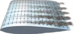
Fig. 1. Conceptual deployment of XDense for active flow control.
Such densely instrumented systems pose however huge challenges in terms of interconnectivity and timely data processing. It is important to note that the need for high spatial and temporal resolutions are often contradictory requirements, which are often not easily simultaneously fulilled. To further motivate our approach, let us consider an aerospace application scenario that may beneit from such dense CPS. The drastic increase in demand for air transportation, naturally motivates measures to reduce its environmental impact. The reduction of fuel consumption is important regarding both environmental efects and cost eiciency. It is known from the Breguet range equation [2] that improvements in aerodynamics, engines, and structure have major impor-tance, and eforts in that direction aim at reducing aircraft drag and weight of the aircraft. In fact aerodynamic drag due to skin friction is known to be one of the relevant factors contributing to increased aircraft fuel consumption, that constitutes approximately one half of the total drag for a typical long range aircraft at cruise conditions [38].
A signiicant part of this skin friction is due to turbulent1airlow over the wing [28]. Turbulence
can be highly undesirable, as it increases drag and noise. Additionally, it causes loss of energy [4], and an important goal is to minimize this loss. Figure 1 exhibits an example in which homogeneous laminar airlow transits to turbulent along the wing.
Several solutions have been proposed already to reduce turbulence. Cattafesta et al. [5] have surveyed the state-of-the-art actuation mechanisms used to reduce turbulent skin friction. A
promising approach is based on a concept known asSynthetic Jet Actuators (SJAs). SJAs are
actuators that run at key positions on the wing and continuously energize the airlow to avoid the formation of turbulence [39]. The recent advances in miniaturization and materials technology enable the development of a (thin) smart skin feasible, and hence SJAs are becoming an achievable
technology [33]. The weakness of SJAs is tonotuse sensors to detect and trace the turbulent lows
and hence ofer only open loop actuation. This compromises the eiciency of active low control (AFC), leading to waste of energy resources when there is no turbulent low or when the turbulence lies outside the actuators' control ield.
Therefore, implementing closed-loop AFC implies that physical quantities are tracked through sensors (for example, pressure, temperature and vibration sensors), which are deployed with some high density (eventually a few centimeters apart). Figure 1 shows an envisioned deployment of such sensing/detecting infrastructure on a wing surface to detect the occurrence of turbulent airlows. XDense was developed to deal with the key challenges related to eXtremely Dense deployments of sensors [20]. XDense has a network architecture composed of regular structures (nodes) in-terconnected in a 2D-mesh network (see Figure 2(a)). This resembles common Network-on-Chip
1Turbulent airlow is composed of coherent structures of chaotic temporal evolution, such as vortices. Turbulent airlow
(NoC) architectures [14] and there are also similarities in routing schemes and distributed comput-ing capabilities [16]. XDense exploits low-cost local communication and distributed processcomput-ing strategies to enable distributed feature detection/extraction.
Even though we focus on AFC as the application scenario in this work, we believe XDense can be useful for other applications that require fast response times and dense networks of sensors. To mention a few: (i) aerodynamic tests [26]; (ii) structural monitoring [30]; (iii) biomedical devices for electroencephalogram [37]; (iv) robotic e-skins [31]; (v) health monitoring wearable sensor networks [25].
To investigate beneits of performing distributed processing, we take into account the nature of the input data. This because the eicacy of data processing algorithm are tightly related to the nature of the input data, in the sense that data clustering strategies and feature detection algorithms must be developed to it speciic scenarios. As well, the spatial and temporal granularity of the input data provides the necessary information to take decisions on the density of the deployment and minimum sampling rate requirements and consequently network load. For example, in [20], targeting AFC, we proposed algorithms to enable distributed turbulent air low detection using computational luid dynamics (CFD) data as our input.
However, the practicality of XDense for eicient feature detection and extraction is a necessary but not suicient condition. We also need to provide execution time guarantees and bounds on the resource utilization for real-time applications like AFC, for which timeliness guarantees are essential to achieve closed loop actuation. Providing bounds on resource utilization is also crucial to correctly dimension the nodes, to avoid overload and consequent data loss. These are factors that have great inluence on hardware requirements, cost and consequently on the applicability XDense. These two properties are therefore the focus of this paper.
Contribution
In this work, we extend XDense with real-time capabilities, by implementing traic shapers in every node such that the network traic is predictable and analyzable. Further, we propose an analysis framework to accurately model the network in terms of communication delay characteristics and memory requirements. Speciically, the paper makes the following two contributions: (i) propose three heuristics to shape the traic in the network; (ii) develop a mathematical framework to model and analyze the application and network and provide upper-bounds on communication delays, application execution time, and maximum bufer requirements.
In extension to the work presented in [18], in this work we evaluate the heuristics proposed using homogeneous and heterogeneous traic sources and compare it with the best efort approach. The remainder of this paper is organized as follows. Section 2 introduces the basics of the XDense architecture; Section 3 formalizes our XDense model for real-time applications; Section 4 evaluates the model; Section 5 discusses the related works and Section 6 concludes the paper along with comments on potential future research directions.
2 XDENSE ARCHITECTURE AND PRINCIPLES OF OPERATION 2.1 Architecture and topology of XDense
(a) Network
N
Tx Rx
Rx Tx
T
x
R
x Tx
R
x
(b) Node
R P
S
ND x4
(c) Node
TS Q
(d) ND
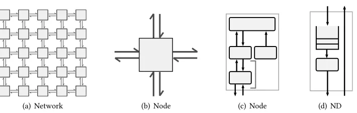
Fig. 2. (a) The XDense 2-D mesh network; (b) nodes use four bidirectional links to connect with neighbors located in the four cardinal directions (North, South, East, West); (c) node internals: processor (P), router (R), net-device (ND) and sensor (S); (d) net-device architecture. Output port includes a queue (Q) and a trafic shaper (TS).
Figure 2 illustrates the components of an XDense network at diferent levels of abstraction. Each node is composed of a sensor (S), a processor (P) and a router (R) and is connected to its neighboring nodes located in the four cardinal directions using bidirectional communication ports; termed networking devices (ND). Because they are bidirectional ports, we refer to their input and output independently as the input ports and the output ports.
The sensor is speciied according to the nature of the phenomena to be monitored. For example, to enable high-precision AFC, pressure and temperature sensors can jointly provide better sensing of the airlow [13].
The processor runs the application layer. It interfaces with the sensor and implements high level application-speciic protocols for data sharing and processing. The router arbitrates the exchange of data. It can receive and transmit packets in parallel, from/to the processor and networking devices. Networking devices are full-duplex serial communication ports. We use serial links as they are widely available in COTS micro-controllers and provide low complexity and low footprint at low cost (compared to parallel links found in NoC[14]). For example, in [8] the authors show that the utilization of parallel links beyond 2 millimeters represent up to 150% larger on-chip area utilization and up to 30% increase in power consumption when compared to high performance serial links. Their results clearly show that serial links present overall better performance compared to parallel links larger than a few milliliters. Thus, we believe that serial links are more appropriate to the deployment scales we envision.
Each one has a queue (Q) and a traic shaper (TS) (see Figure 2(d)). Input packets are directly delivered to the router whereas output packets are irst queued (in FIFO order) at the target output port before they are dequeued by the traic shaper to be then transmitted serially over the network. All network transfers are non-preemptive and packet-switched, and all packets have a ixed and equal size.
The purpose of the traic shaper is to provide determinism to the output traic, and consequently make it amenable to real-time analysis. Its function is two-fold: it implements a release ofset to the output packets and makes the transmission periodic. Shaping the traic enables us to formulate the output traic as a linear cumulative function of the input traic. We will discuss our traic shaping techniques in detail in Section 3.
[image:5.486.68.423.84.197.2]2.2 Hardware implementation
Temperature UART N
JTAG
I2C
µC
Light
9D motion Pressure
UART E
UART S UART W
UART DBG
Onboard components Interfaces
(a) (b) (c)
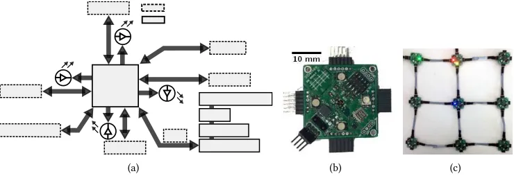
Fig. 3. (a) node’s schematic showing each major components of the system. (b) Node prototype. (c) 3×3 network.
For realizing the above design of XDense, a custom design integrated circuit (IC) provides the best-it solution; But this reduces design lexibility and might become a single application solution.
For this reason, we use a microcontroller (µC) and other COTS to prototype the XDense node and
network. The rest of this section provides context to this discussion with a short overview of the prototype that we have developed, shown in Figure 3.
To implement XDense, we chose the Atmel ATSA℧4N8AµC. It is based on the 32-bit AR℧
Cortex-℧4 RISC processor, which is a mid-range general purposeµC, that runs at up to 100 ℧Hz
and provides a good balance between power consumption and processing power. It has a small 48 pin footprint, with ive high speed UART ports, each with dedicated D℧A channels that allows eicient communication. We use the FreeRTOS[3] real-time operational system (RTOS) in our nodes. It provides device drivers and additional high level abstractions for context switching and multi tasking.
The schematics, prototype node and a 3x3 network deployment is shown in Figure 3. We placed four sensors on the top of the board for: motion sensing with 9 degrees-of-freedom; pressure; temperature, and visual-range light sensing. We have presented more details on the hardware prototype using COTS in [19].
2.3 AFC application scenario
We now revisit the AFC application discussed in the introduction. While not used as input in the analysis ahead, the focus being to prove the realtime nature of XDense, it is useful to understand how XDense its into the AFC application worklow.
As shown in Figure 1, XDense is positioned on the wing of the aircraft to collect the environment data. Experimentally, a wind tunnel would be desired to pose the aerodynamic conditions over a wing surface embedded with an XDense network. Computational Fluid Dynamics (CFD) simulation allows us to simulate airlow over a wing and collect this information by a virtual deployment of XDense. This is a well studied area in aerodynamic research and one important test case is for the
ONERA ℧6 wing in viscous low [32].2
2The ONERA ℧6 wing was designed for studying three-dimensional, high Reynolds number lows with complex low
[image:6.486.59.429.118.245.2](a) (b) (c)
0 5 10 0
5 10 15 20 25 30
(d)
Fig. 4. (a) Pressure distribution over a wing’s surface. (b) Data of a single time-frame, from Computational Fluid Dynamics (CFD) simulation, as input for XDense. (c) Sensors displacement; (d) Normalized data, as seen by each sensor.
We have integrated this CFD simulator into our worklow for simulation of XDense inputs. Now, the AFC input simulation worklow consists of the following steps:
(i) Generate wing model:A 3D mesh of a wing is generated and imported into the CFD simulator (Figure 4(a));
(ii) Simulate wing performance:The CFD simulator is run to simulate a pitching wing lowing through high speed air low. Temporal pressure and temperature data of the surface of the wing are produced. (Figure 4(b));
(iii) Extract sensor data:These temporal pressure and temperature data are extracted, but only
from the points in space that correspond to the XDense node deployment. Figures 4(c) and 4(d) illustrate sensor deployment and sensor data, respectively.
℧ore speciically, the sensor data is generated and imported using the SU2 simulator for multi-physics [24]. SU2 is a reliable open-source CFD simulator which is widely used in aerodynamics research.
Even though we integrate our simulation model and the SU2 CFD simulator, note that the input data is indiferent to the network operation, as the analysis pertains to the communication aspects only. Therefore not inluencing in any way the results presented in this paper.
2.4 Principles of XDense Operation
Consider the AFC use case depicted in Figure 1 as a working example. The objective is to col-lect information on the nature of the airlow and identify whether it is laminar or turbulent by quantifying its characteristics along the wingspan.
A naive solution to this problem is to request each node to continuously sense information about the airlow and send it back to a sink. The information collected from the sink can then be used to compute the airlow's properties. Clearly, this approach generates a tremendous load on the network, requires large bufers in each node, and leads to signiicant delays between the time at which the information is requested and the time at which it is eventually processed (sensed information may have a maximum lifetime).
[image:7.486.50.433.82.241.2](d) (b)
(c) (a)
[image:8.486.47.440.87.211.2]Input flow Output flow
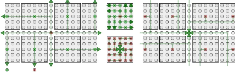
Fig. 5. Example45×45network, with a single central sink. In this case, withnradius=2. Application phases:
(a)ϕ1ś Sink requests data from cluster-heads; (b)ϕ2ś Cluster heads in turn send a multicast request to nodes in their cluster; (c)ϕ3ś Nodes send sensor data back to their respective cluster-head; (d)ϕ4ś Cluster heads process received data and send result to sink.
head node. It performs data aggregation within its cluster and is responsible for processing (and/or compressing) the data locally to send only meaningful information to the sink. Another example
of utilization is to program the cluster heads to inform the sinkonly upon the occurrence of
meaningful events (e.g., airlow changes from laminar to turbulent and conversely).
The routing protocols elected should ideally exploit the network topology to avoid congestion. It is also required to deine application protocols to allow coordination of clusters by the sink.
To tackle the challenge of analyzing and computing upper-bounds on the application execution time and the bufer requirements of the nodes through distributed processing, XDense uses three operative principles: (1) the nodes are clustered and one node in each cluster (cluster head) is in charge of aggregating and pre-processing the data; (2) the execution of the application is divided logically in subsequent phases; (3) the network implements routing schemes which guarantees spatial isolation between the clusters.
2.4.1 Clustering nodes.The reason for grouping the nodes into clusters is to reduce the load on the network by performing in-cluster data pre-processing at the selected cluster heads. Our tested solution implements non-overlapping łsquarež clusters ś the network topology being a 2D grid
ofX timesY nodes, all clusters are non-overlapping and of sizensize×nsize, withnsize ≤X and
nsize≤Y.nsizemust be a positive odd number and the cluster head is the node located at the łcenterž
of the square. The cluster sizensizeis deined through the system parameternradiusthat denotes the
maximum distance from the cluster head to the farthest node in the cluster (considering rectilinear
distance, a.k.a. ℧anhattan distance). Figure 5 shows a scenario withnradius=2. Thus, the resulting
total number of nodes in each cluster is a function of thenradiusgiven by(2×nradius+1)2.
Nodes arbitrate their role on the network at run time (to act either as cluster head or normal node). They do this on reception of a packet from the sink containing the packet origin and the
nradiusparameter. Each node then calculates, based on its position in the network relative to the
sink, if it is supposed to act as a cluster head or as a normal node.
discussed application speciic data processing issues in previous works (see [20] for a discussion on this topic).
2.4.2 Executing application in phases.The execution of the application is logically divided into
a set of four consecutive phasesϕ1,ϕ2,ϕ3andϕ4. The irst phase is started by the sink, when it
requests data from the cluster heads. Speciically, the four phases are:
• Phaseϕ1. The sink requests the cluster heads of all clusters to send the processed data;
• Phaseϕ2. On receiving the request from the sink, the cluster heads in turn request the nodes
of their respective clusters to send their data;
• Phaseϕ3. Every node of each cluster transmits its sensed data to its cluster head;
• Phaseϕ4. The cluster heads process the received data and transmit the result back to the sink.
Note that the clusters maynotalways be in sync with respect to the phase of their execution.
The second phase (ϕ2) for instance, start in each cluster with a diferent time ofset; This ofset
being proportional to the distance between the cluster head of each cluster and the sink. We assume
cluster heads' clock are synchronized duringϕ1, at the time they receive the request from the sink.
The same applies to sensor node's clock, which are synchronized duringϕ2, at the time they receive
the request from their cluster head. That is, all nodes co-participating on a phase (in the same cluster) have a common time basis, which is an important assumption for the proposed heuristics to work. We believe this is a reasonable assumption, since nodes synchronization point happen just before synchronism is required, providing a momentary synchronism during a given phase, even when there is considerable clock skews between nodes.
Despite their special role, the sink and cluster heads sense as any other node. The sink is the only node to act as the gateway with the outside world and has a backhaul link (for example, a wireless link). Figures 5(a) to 5(d) show the four phases in a chronological order.
2.4.3 Spatial isolation through routing schemes.The four phases described above require spatial isolation so that packets do not compete with each other for network resources when traversing it. We use the well-known dimension-order routing algorithms known as X-Y and Y-X routing protocols [14]. In X-Y routing (resp, Y-X), packets are irst routed along the X (resp, Y) dimension and then along the Y (resp, X) dimension. These protocols always ind the shortest path between the source and destination nodes (again, in terms of the ℧anhattan distance) and are proven to be deadlock-free [11].
Phasesϕ1toϕ3use one of the following two routing algorithms, sometimes called
Counterclock-wise Dimension Routing (see Figures 5(a)-(c)). The starting dimension (X or Y) depends on the
quadrant in which the destination node is, relatively to the origin of the packet. For phaseϕ4we
propose another routing protocol hereafter referred to as Shifted Clockwise Dimension Routing. This protocol adds an initial change in dimension on the irst hop and then uses a regular clockwise routing (see Figure 5(d)).
The nodes aligned with the sink are not part of any cluster. They provide an exclusive route for
packets ofϕ4, sent by the cluster head to the sink. This routing scheme results in lows from phase
ϕ4to travel orthogonal to the lows from phasesϕ1,ϕ2andϕ3and therefore they do not compete
for the same output port at any node on the way. This enables spatial isolation between the lows from the diferent phases.
3 EXTENDING XDENSE WITH REAL-TIME APPLICATION CAPABILITIES
We endow XDense with real-time capabilities byshaping the traic at every output port of every
f1
f2
R TS f3
ND
Node 25 20 15 10 5 0
0 5
10 15
TTS
[image:10.486.48.445.84.125.2]TTS
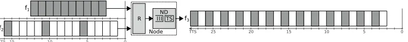
Fig. 6. Trafic shaper example scenario: two input flows shaped by an intermediate node as an output flow. Parameters for the input flows aref1={O=2.5,β=1,σ=10}andf2={O=1,β=15,σ =3}. The resulting flow isf3={O=2,β=12,σ=13}.
we are able to compute the maximum bufer requirement and determine precise upper-bounds on the application execution time.
3.1 Networking model
The real-time application deployed on the network is characterized by a setΦ={ϕ1,ϕ2, . . . ,ϕn}of
nconsecutive event-triggered phases (communication and processing primitives) that constitute
the logical part of the application execution. In this work, we assumen=4 (as explained in the
previous section) but the approach can be extended to any arbitrary numbernof phases. Every
phaseϕi ∈Φ, withi ∈[1,n], is characterized by a setFi ofmi ≥1 communication traic lows
exchanged between the nodes involved in phaseϕi. Each lowfi,j ∈ Fi, withj ∈[1,mi], consisting
of one or more packets, has an unique source node from which the communication is initiated, and
may have multiple destination nodes. Formally, a lowfi,jis modeled as:
fi,j ={Oi,j , σi,j, βi,j} (1)
The ofsetOi,j is a constant delay before the sending of the irst packet of lowfi,j. The message
sizeσi,j is the number of packets that are sent in each lowfi,j and the burstinessβi,j ∈ [0,1]
represents the rate at which those packets are released. A burstiness of 0 means that no packets
are transmitted, and a burstiness ofx ∈ ]0,1] means that a packet is transmitted every 1
x TTS.
These three parameters together describe a inite constant-rate low with an initial ofset. The low
parametersσ andβ were conceived to couple the application sampling requirements with the
communication model, in the sense that they allow modeling application scenarios with diferent data sampling requirements. A few example lows are illustrated below.
Example 3.1 (9 Degrees of Freedom (DOF) motion sensor). Consider a 9 DOF motion sensor whose
data has to be transmitted as nine separate packets in a single low (one packet for each degree of
freedom). In this case, we want the data to be transmitted together. Therefore, we setβ =1 with
σ =9 for that low.
Example 3.2 (Pressure sampling). Consider a use-case in which ten samples of pressure data need
to be transmitted, using one packet per sample. We are interested in having periodic sampling,
equally distributed in time. By setting the burstiness to15 for instance, one packet will be sent every
5 TTS. Therefore, for that low we setβ= 15andσ =10.
3.2 Shaping flows and trafic throughout the network
As discussed above, the sending of all packets by the source node of the corresponding lowf is
done according to its parameters (O,σ,β); these three parameters allow for a precise timing and
sending rate at the source node off. Note that for simplicity, we shall use hereafter the symbol
f to denote a low. We will mention the indexesiandjthat indicate the phase and low indexes
Although the lows are shaped at their source, when multiple lows (say,f1in,f2in, . . . ,fkin) traverse the network at the same time, pass through the same router, and compete for the same output port,
the resulting output lowfoutat that port is a superposition of all these competing lows. As such,
foutmay present an irregular packet transmission pattern and a rate that can no longer be modeled
using the three parameters (O,σ,β).
For example, let us look at Figure 6, which illustrates two input lowsf1inand f2incompeting for a
same output port of a node. Each of these lowsfkinstarts at timeOkand has a duration deined as
ℓk= σk
βk. That is, lowfksends all its packets afterℓk TTS, att=Ok+ℓk. In this example, thanks
to the traic shaperTS, the interference of these two input lows lead to an output lowf3outthat is
not a superposition of the two input lows, but rather it preset deterministic patterns that can be
modeled using the three parameters (O,σ,β).
That is, to make the network amenable to timing analysis, we shape the traicat every output
portof every node and make it it the linear model (O,σ,β). For that, we irst identify the set of
input lowsfkin(withk =1,2, . . .) at every output port of every node in the network, and based on
the respective parameters (Ok,σk,βk) of these lows, we compute the parameters (Oout,σout,βout)
that are used to shape the resulting output low at that output port.
In Figure 7, we present a more detailed example to illustrate how the traic shaping is done.
Figure 7(a) shows packet arrivals curveS(t)due to four incoming lows f1in,f2in,f3inand f4in(see
Figure 7(b)). The arrival curve correspond to the incoming lows that deine the number of packets to be sent over time from the output port, that depends on the starting time and duration of all the
competing input lows. Three possible resulting lowsfoutare computed and shown in Figure 7(c),
each with its corresponding departure curve in Figure 7(a).
The computation of (Oout,σout,βout) is therefore performed at every output port of every node
in the network interactively, starting at the source node of every low and iterating, one port at
the time, throughout the network until a shaper is deined for all the output ports.3We make two
important assumptions regarding the lows and their routing.
Assumption 1.During phasesϕ3andϕ4, in every node, all the packets entering by a given
input port are assumed to exit through a single output port.
Assumption 2.There are no circular dependency between the lows. For any output port, say
p1, the computation of the parameters of its traic shaper requires each of its competing input
lows to be modeled already by the three parameters (O,σ,β). If any of these input lows, say
fkin, comes from the output port (sayp2) of an upstream router, it is required that the parameters
(Okin,σkin,βkin)of the shaper of that upstream output portp2have been computed already. Similarly,
this requirement must be satisied for all the input lows competing forp2, and interactively it
must be satisied as well for all the output ports of the upstream routers till the traic shaper at the source nodes of all the interfering lows. Therefore, computing traic shaping parameters is an
iterative process that must be executed until (Oout,σout,βout) is calculated for all nodes. In simple
terms, there cannot be a lowf1competing for an output port with a lowf2that competes for an
output port with a lowf3, and so on until reaching a lowfkthat competes for an output port with
f1.
Assuming no cyclic dependencies between the lows, the parameters (Oout,σout,βout) of every
traic shaper may be computed in many diferent ways for a same set of interfering input lows. In the next section, we propose three diferent methods of computation.
3Note that it has been proven in [35] that to calculate optimal shaping parameters in a multihop scenario can be
S(t) Min-O Max-S LQ
oLQ oMin-O oMax-S
βMin-O
Time (t)
P
a
c
k
e
t
c
o
u
n
t
(n
)
βMax-S
p1
p2 p3
p4
p5
p6
p7
p8
f1 f2
f3 f4
(a)
(b)
Time (t) βLQ
fMin-O
fMax-S
Time (t)
(c) f
[image:12.486.123.363.84.262.2]LQ
Fig. 7. Trafic shaping heuristics: (a) input, and output flows using the proposed heuristics; time-line showing ofset and duration of (b) arriving flows and (c) departure flows.
3.3 Shaping output trafic at a single output port
We propose three heuristics to compute the parameters(Oout,σout,βout)of the shaper used at a
given output port. LetFindenote the set of input lows that compete for the output port under
analysis. Everyfkin∈Finis characterized by the three parameters(Okin,σkin,βkin). For eachfkin∈Fin,
we deine the functionSkin(t)as
Skin(t)=
0 t ≤Okin
βink ×(t−Okin) Oink <t<Okin+ℓk
σkin t ≥Okin+ℓk
(2)
Broadly speaking, every functionSink(t)represents the number of packets sent by the lowfkinat a
given timet(TTS). Whentis earlier than the starting instantOkinof the low, the function returns
0 since the low has not sent a packet yet; Fortlarger than the inishing time of the low (Okin+ℓk),
the function returns the total numberσkinof packets sent byfkin, withℓkbeing the duration of the
low; Between the two boundsOkinandOkin+ℓk, the function increases steadily from 0 toσkinwith
a constant slope ofβkin.
LetS(t) = Pfkin∈FinSkin(t) be the sum of the functionsSkin(t) of all the input lows fkin. This
functionS(t)is depicted in Figure 7(a). Informally,S(t)gives the number of packets that arrive at the
considered input port in a time window of lengtht(TTS). We further denote byT ={t1,t2, . . . ,tm}
the inite set of time-instants (sorted in chronological order) corresponding to the discontinuity
points of the functionS(t). These discontinuity points are denoted asp1,p2, . . . ,pmin Figure 7. With
these new notations, we can introduce our three heuristics for the computation of the parameters
(Oout,σout,βout)of the shaper used at the analyzed output port.
For a given shaper(Oout,σout,βout)represented by a straight lineLoutof slopeβoutand passing
through the point(Oout,0), theverticaldistance dvoutj between a point(tj,S(tj))∈S(t),∀tj ∈ T,
and the lineLoutrepresents the number of packets being bufered at timetat that output port. The
(induced by the shaper) that all the packets that have arrived at that output port at timetj will
incur because of the shaper.
We start by computing the output low sizeσoutthat is the same for all the heuristics proposed.
Since the shaper is not allowed to drop any packet, it is naturally the sum of the size of all the input
lowsfkin, i.e.
σout=
X
fkin∈Fin
σkin
In the remainder of this section we discuss the intuition behind each heuristic and explain how
they derive the two other low parameters,Ooutandβout.
3.3.1 Minimum ofset (℧in-O).This irst heuristic aims at avoiding bursty traic while coping as much as possible with the bandwidth demand of the input lows. This traic shaper forwards the
irst packet as soon as it can, i.e. one TTS after the packet has arrived, at timeOout=t1+1 TTS,
and forwards all the subsequent packets at the highest admissible rate; that is, with the highest
burstinessβoutsuch that the number of packets sent at any timet ≥ Ooutnever exceedsS(t).
This burstiness corresponds to the highest slope among the slopes of all the lines passing through
the point(t1+1,0)such that, for everytj ∈ T, the point of x-coordinatetj in the line has an
y-coordinate≤S(t)ś In simple terms, the line is łbelowž the functionS(t),∀t ≥0. This slope is
simply given by
βout= "
min
tj∈ T
S(tj)
tj−(t1+1)
!#1
0
where [x]z
y =max(min(x,z),y). Note that by deinition oft1, we havet1 =minfin
k∈Fin(O
in
k).
Fig-ure 7(a) shows ℧in-O departFig-ure curve withβoutasβ℧in-O.
3.3.2 Maximum slope (℧ax-S).The second heuristic aims atnotconsuming any bandwidth for as much time as possible and then send all the packets in a burst. Similarly to the ℧in-O heuristic,
the ℧ax-S approach selects one łanchorž point ofS(t)and computes themaximumslopeβoutsuch
that the line with slopeβoutpassing through the selected point is łbelowž the functionS(t). In
℧in-O, we selected the anchor point(t1+1,0)whereas ℧ax-S selects the point(tm,S(tm)). The
maximum admissible slope such that the line remains belowS(t)is given by:
βout=max tj∈ T
S(tm)−S(tj)
tm−tj
!
(3)
Figure 7(a) shows ℧ax-S departure curve withβoutasβ℧ax-S. The ofsetOoutin ℧ax-S is simply
set to the X-intercept of the line of slopeβoutand passing through the anchor point(tm,S(tm))to
which we add 1 TTS, to make sure that packets are not forwarded before the irst packet arrives (like we did in ℧in-O), i.e.
Oout=tm−
S(tm)
βout +1
After computing the ofsetOout, it is now safe to readjust the slope asβout=βout10to model the
fact that the shaper cannot forward a negative number of packets and neither it can forward more
than one packet at a time. Note that this re-adjustment must be performed after computingOoutas
doing it before would in some cases allow a packet to be forwarded before it even arrived, that is,
Figure 7(a) shows the departure line of ℧ax-S, initially calculated with a slope>1 as a result
of Equation 3. That slope is then adjusted toβout=1 as depicted on that Figure. As seen, after
adjusting its slope, the line corresponding to the parameters of the ℧ax-S traic shaper does not
intersect with the functionS(t)ś It seems to be łtoo much shifted to the rightž. An easy patch to
reduce this gap betweenS(t)and the shaper is to set its ofset to theminimumofset such that the
line remains below all the points ofS(t). That is,
Oout=min t≥0
tsuch thatβout ≤min tj∈T
tj>t
S(t)−S(tj)
t−tj
!
(4)
Note that this value ofOoutcan be computed easily by positioning the line of slopeβouton every
point(tj,S(tj)),∀tj ∈ T, and retaining the maximum X-intercept of all these lines.
3.3.3 Least-square regression (LQ).The intuition behind this third heuristic is to minimize both
the queue size and the delay by inding the lineLoutthat minimizes the distance between every
point(tj,S(tj))∈S(t),∀tj ∈ T andLout. This line is commonly known as theregression lineof the
points(tj,S(tj)) ∈S(t). Using the least-squares method, which is the most common method for
itting a regression line, the slope of that line is given by
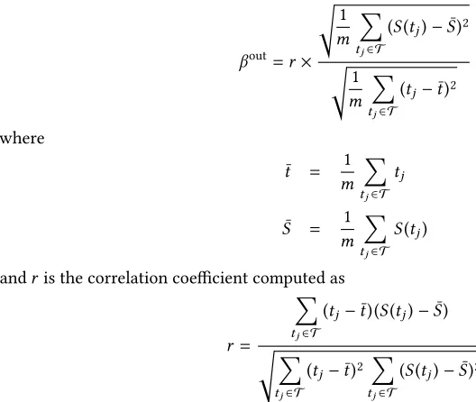
βout=r×
s 1
m
X
tj∈ T
(S(tj)−S¯)2
s 1
m
X
tj∈ T
(tj−t¯)2
(5)
where
¯
t = 1
m
X
tj∈ T
tj
¯
S = 1
m
X
tj∈ T
S(tj)
andr is the correlation coeicient computed as
r =
X
tj∈ T
(tj −t¯)(S(tj)−S¯)
sX
tj∈ T
(tj−t¯)2
X
tj∈ T
(S(tj)−S¯)2
Once we have computed the slope, we choose the smallest ofsetOoutsuch that the line of slope
βoutand passing through(Oout,0) is never above any point(t,S(t)),∀t ≥0. This is done using
Equation 4.
3.4 Worst-case per-hop delays and maximum queue sizes
Having stated the heuristics, we can now apply them to all the phases of the application. We perform this in a hop-by-hop strategy, starting from the output ports of the nodes for which the
parameters(Okin,σkin,βkin)of all the interfering lowsfkinare known. For each such output port, the
resulting output lowfoutis shaped using the same model(Oout,σout,βout)that is then propagated
[image:14.486.46.310.310.533.2]every output port of all the nodes of the network are deined (the output ports that no lows ever traverse and that are thus unused are naturally ignored). As mentioned earlier, we assume that there are no cyclic dependencies between the lows at any output port, which implies that the process eventually terminates.
After that step, we can now compute at each output port the maximum transmission delay caused
by its traic shaper(Oout,σout,βout), as well as its maximum queue size. To ease the explanation,
we shall use the same visual representation as that used in the previous section for the shaper and
the functionS(t). The shaper is represented by a straight line of slopeβoutthat intersects with the
x-axis at the point(Oout,0). We denote this lineLoutand write its equation as
Lout(t)=βoutt−βoutOout (6)
We deineS(t)as in the previous section and keep the notationsT ={t1,t2, . . . ,tm}to express the
inite set of time-instants (sorted in chronological order) corresponding to the discontinuity points
of the functionS(t).
As explained previously, the number of packets bufered at the output port at any time-instantt
is given by theverticaldistance dvoutj between the point(t,S(t))and the point(t,Lout(t))on the
lineLout. This vertical distance is simply equal to
dvoutj =S(t)−Lout(t)
and thus the maximum number ℧axueue of packets bufered at that output port is given by
℧axueue=max
t≥0
S(t)−Lout(t)
SinceS(t)is a continuous piecewise function for which every sub-function is linear, it can easily
be showed that the maximum of the previous equation can be found by looking only at the
time-instantstj ∈ T rather than at allt ≥0, i.e.,
℧axueue=max
tj∈ T
S(tj)−Lout(tj)
(7)
This holds true because every sub-function ofS(t)is a segment that is either:
• parallel toLout. In this case, all the points on that segment are at the same distance fromLout,
including its two extremities that are discontinuity points with an x-coordinate included in T.
• converging towardsLout. In this case, theleftmostpoint on the segment (whose x-coordinate
is an instanttj ∈ T) is the furthest toLout.
• diverging fromLout. In this case, therightmostpoint on the segment (whose x-coordinate is
an instanttj ∈ T) is the furthest toLout.
Similarly, the transmission delay at any time-instanttis given by thehorizontaldistance dhoutj
between the point(t,S(t))and the point of y-coordinateS(t)on the lineLout. According to
Equa-tion 6, that point of y-coordinateS(t)∈Louthas an x-coordinatexsuch thatS(t)=βoutx−βoutOout
and thusx= Sβ(outt) +Oout. The horizontal distance is then simply given by:
dhoutj =
S(t)
βout+O
out−t
and thus the maximum delay ℧axDelay at that output port is:
℧axDelay=max
t≥0
S(t)
βout +O
out−t
0 5 10 15 20 25 30 Transmission time slot (TTS) 0
2 4 6 8
Cumulative packet count
SIM Min-O Delay Queue
(a)
0 5 10 15 20 25 30 Transmission time slot (TTS) 0
2 4 6 8
Cumulative packet count
SIM Max-S Delay Queue
(b)
0 5 10 15 20 25 30 Transmission time slot (TTS) 0
2 4 6 8
Cumulative packet count
SIM LQ Delay Queue
[image:16.486.57.436.91.215.2](c)
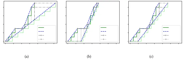
Fig. 8. Cumulative arrival/departure curves for a single node, using (a)℧in-O, (b)℧ax-Sand (c)LQheuristics.
For the same reasons as those mentioned for ℧axueue, the maximum delay ℧axDelay can be
computed by looking only at the pointstj ∈ T, i.e.,
℧axDelay=max
tj∈ T
S(tj)
βout +O
out−t
j
!
(8)
Note that the transmission delay is an interesting parameter to analyze the end-to-end delay or per-hop delays of individual packets. However, in this paper we rather focus on estimating upper-bounds on the execution time of the phases and thus of the overall real-time application.
To compute the execution time of a given phase, we must know exactly when the phase start and when it ends. However, phases may overlap in time and happen simultaneously. For instance, for the application scenario considered in this paper, a cluster head located close to the sink may
enter phaseϕ2long before a cluster head that is far from the sink (since it receives the request from
phaseϕ1sooner). For simplicity, we assume in this work that a phase ends when a given node has
received all the packets sent to it. For example, the time at which all the cluster heads have received
their requested data marks the end of phaseϕ3and the time at which the sink has received all the
processed data marks the end of phaseϕ4. As such, we compute the execution time of a phase as
the relative time-instant at which all the four input lows of that given node ś a cluster head for
phaseϕ3and the sink for phaseϕ4ś terminate, i.e. the four lows coming from the north, south,
east, and west input ports of that node. The execution time of a phase is thus given by
ExecTime= max
card∈[↑,↓,→,←] O
in +σ
in
βin
!
(9)
where for each cardinal direction↑,↓,→, and← (north, south, east, and west), the low fin
characterized by(Oin,σin,βin)is the input low coming from that cardinal direction.
3.5 Validation example
To validate our theoretical model we compare it with simulation. For that, we deine the following scenario: a single node receives an arbitrary number of known input lows, which are shaped into an output low (using any of the proposed heuristics) We compare the arrival/departure curves calculated using our model, against the curves obtained in simulation.
We use the same input lows in all three scenarios, which areFx =[f1in,f2in,f3in], wheref1in =
{O =0,σ =3,β =0.5}, f2in ={O =10,σ =3,β =0.5}andf3in ={O =12,σ =3,β =0.5}. The
resulting output lows are diferent for each heuristic, which arefMinout−O ={O=1,σ =9,β=0.3},
fout
M ax−S={O=8.2,σ=9,β =0.83}andfLQout ={O=4.8,σ =9,β=0.49}.
The arrival curves obtained through simulation (common to the three cases) is a stair function that presents the superposition of all the arriving lows. Because the output low is shaped, the corresponding departure curve is a homogeneous stair function. As expected, the arrival/departure curves calculated using our model precede the simulated ones in every point. It also shows the queue size and delay calculated at every point in which the arrival and/or departure curves start, inish or change its slope.
For the givenFx, from Figure 8(a), ℧in-O performs badly compared to the other heuristics, as it
adds large delays between the arrivals and departures, which leads to equally large queues and long execution time. We notice from Figure 8(b) that the departure curve obtained with ℧ax-S approaches maximally the arrival curve at its tip (1 TTS far), leading to the optimal execution time with the cost of larger queues from 0 to 10 TTS. On the other hand, LQ heuristic leads to smaller queues, with a slightly longer execution time.
Although these results provide an intuition on the trade-ofs between the heuristics proposed, they do not depict the results of multi-hop communication, in which case the efects may difer. Therefore, a more complete evaluation is provided in the next section to understand how each heuristic performs through multiple hops.
4 EVALUATION OF TRAFFIC SHAPING HEURISTICS
Application use-case:To evaluate the proposed heuristics, we consider the application scenario introduced in Section 2. Remember that the execution of this application is divided logically in
four consecutive phasesϕ1,ϕ2,ϕ3andϕ4. In the irst phaseϕ1, the unique sink node requests all
the cluster heads to send their data; in phaseϕ2, the cluster heads performs another request to all
the nodes of their respective cluster; in phaseϕ3, the nodes reply to the cluster heads by sending
them the sensed data; and in phaseϕ4, the cluster heads process the data received and transmit
the result back to the sink. Since there is no network congestion in phasesϕ1andϕ2ś because all
the packets sent from the sink to the cluster heads and then from the cluster heads to the sensing nodes have their own private route to their destination ś these two phases are neither afected by a modiication of the cluster size, nor by changing the number of clusters, nor by altering
the burstiness of the lows generated during phasesϕ3andϕ4. We shall therefore focusonlyon
phasesϕ3andϕ4in which network congestion does occur and for which a modiication of the
aforementioned parameters has an impact on the performance.
Network setup:The network is organized as a square grid of 45×45=2025 nodes with an
unique sink located at the center of the grid. Figure 5 depicts a closeup on the sink. In that igure we can also see the overall cluster organization, the routes taken by the lows in the diferent phases and the central row and central column of nodes in the middle that are dedicated only to
the communication between the cluster heads and the sink. Based on an integer parameternradius
that we vary in our experiments, we deine every cluster as a square grid of(2nradius+1)2nodes
with the cluster head at the center of the grid. As such,nradiusdeines both the cluster size and
Shaping heuristics:We evaluate the performance of the three proposed heuristics ℧in-O, ℧ax-S, and LQ against the performance of a cycle-accurate network simulator that we call BE. The simulator does not implement any traic shaper and thus it delivers the best efort (BE) performance overall.
Simulator:The simulator consists of a module for XDense on top of Network-Simulator-3 (NS-3). It is scalable to simulate very large network deployment scenarios with low computational cost. This is because we use packets, routing algorithms and addressing schemes with low overhead, tailored to this kind of network.
The general nature of the design and implementation of conigurable links, packets, communi-cation ports, router and applicommuni-cations, also makes our module suitable to other 2D mesh network architectures as well (NoCs for example). This is because the diferent abstraction levels can be implemented independently, as a set of intermediate models, each one with its speciic objectives. For example, the traic shapers theorized in this work were actually implemented in our simulator as an independent application layer, so we could study its practical viability, and for debugging
purposes.4
Evaluation criteria and methodology:For each of the three heuristics ℧in-O, ℧ax-S, LQ, we
evaluate the maximum queue sizes and the end-to-end execution time of the phasesϕ3andϕ4. For
BE, maximum queue sizes and phases execution time are measured in the simulator. We do so for diferent cluster sizes, low burstiness and network load distribution. Because there is no source of nondeterminism in our simulation model, each runs gives the exact same results for the same input parameters. Thus, we are only required to run our experiments once for each scenario, for as long as all four phases last.
To understand the impact of varying the network load, we analyze both homogeneous and
het-erogeneous low scenarios in phasesϕ3andϕ4(that is, the phases when the actual data transmission
happens). We deine a homogeneous low scenario as one in which all nodes generate lows with equal burstiness and message size. A scenario with random message sizes and burstiness is deined as a heterogeneous low scenario.
We analyze the homogeneous scenario by varying the burstinessβof lows from phasesϕ3and
ϕ4from 0.02 to 1 by step of 0.02, for diferent cluster sizes.
The message sizeσ difers for each phase. For phasesϕ1andϕ2, a single packet is generated
at the sink and cluster head (σ = 1). In phaseϕ3, each node outputs a low with message size
σ =4. At the end ofϕ3, the cluster head receives in total four packets per each node on its cluster.
Subsequently, each cluster head outputs a low with message sizeσ, as the sum of all these packets
plus 4 packets of its own sensed data, times⌈1−CR⌉. The term CR aims at reproducing the efect
of data compression by the cluster head. For this work we deine this as a ixed value equal to
CR = 80%, which was shown in previous work [20] to be a reasonable ratio in some air low
scenarios. The number of packets originated by each cluster vary with cluster size, whereas the number of clusters is inversely proportional to the cluster size. This trade of has a compensatory efect on the overall number of packets transmitted to the sink.
In the heterogeneous low scenario, lows generated at phasesϕ3andϕ4have random message
sizes. We use a uniform distribution function withσ =rand(0,10)and burstinessβ=rand(0.02,1).
A message size of zero signiies that a node does not have an output low.
In our results, we compare the performance of both heterogeneous and homogeneous scenarios. In order to do this fairly, we guarantee that for both homogeneous (HO) and heterogeneous (HE) network load distribution, the sum of burstiness of all lows, as well as the sum of all message sizes,
4The simulator source code used in the simulation this paper for the simulator, pre and post processing tools, example
0.0 0.2 0.4 0.6 0.8 1.0 Burstiness ( )
0 10 20 30 40
Max queue size
Min-O Max-S LQ BE
(a) ϕ3,nradius=1
0.0 0.2 0.4 0.6 0.8 1.0
Burstiness ( ) 0
10 20 30 40
Max queue size
Min-O Max-S LQ BE
(b)ϕ3,nradius=3
0.0 0.2 0.4 0.6 0.8 1.0
Burstiness ( ) 0
10 20 30 40
Max queue size Min-OMax-S
LQ BE
(c)ϕ3,nradius=5
0.0 0.2 0.4 0.6 0.8 1.0
Burstiness ( ) 0
10 20 30 40
Max queue size
Min-O Max-S LQ BE
(d)ϕ4,nradius=1
0.0 0.2 0.4 0.6 0.8 1.0
Burstiness ( ) 0
10 20 30 40
Max queue size
Min-O Max-S LQ BE
(e)ϕ4,nradius=3
0.0 0.2 0.4 0.6 0.8 1.0
Burstiness ( ) 0
10 20 30 40
Max queue size
Min-O Max-S LQ BE
[image:19.486.49.438.88.350.2](f)ϕ4,nradius=5
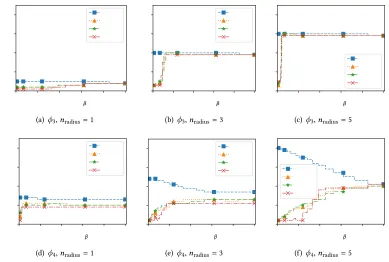
Fig. 9. Homogeneous flow scenario: Maximum queue size for trafic shaping heuristics against simulation. Results are for phasesϕ3andϕ4andnradiusset to1,3and5.
(a) BE,ϕ4,nradius=5 (b) LQ,ϕ4,nradius=5
Cluster head Sink
Cluster
Fig. 10. ueue size density map of the top-right quadrant of the network (17×7 nodes), for heuristics (a)LQ
and (b)BE. X and Y axis are nodes coordinates relative to the sink.
are equal. That is,P
βH O =PβH EandPσH O =PσH E. This guarantees that the total network
load remains the same for both scenarios, even if individual load distribution varies.
For both scenarios, the ofset remains the same; and equal to their distance from the sink/cluster head (since it is meant to model the minimum time required for a node to reply to a request).
4.1 Maximum queue size with homogeneous load distribution
For each of the three heuristics ℧in-O, ℧ax-S and LQ, we irst derive the parameters(O,σ,β)of
[image:19.486.54.435.409.502.2]0.0 0.2 0.4 0.6 0.8 1.0 Burstiness ( )
0.0 0.2 0.4 0.6 0.8 1.0
Link utilization Min-OMax-S
LQ BE
(a) ϕ3,nradius=1
0.0 0.2 0.4 0.6 0.8 1.0
Burstiness ( ) 0.0 0.2 0.4 0.6 0.8 1.0
Link utilization Min-OMax-S
LQ BE
(b)ϕ3,nradius=3
0.0 0.2 0.4 0.6 0.8 1.0
Burstiness ( ) 0.0 0.2 0.4 0.6 0.8 1.0
Link utilization Min-OMax-S
LQ BE
(c)ϕ3,nradius=5
0.0 0.2 0.4 0.6 0.8 1.0
Burstiness ( ) 0.0 0.2 0.4 0.6 0.8 1.0
Link utilization Min-OMax-S
LQ BE
(d)ϕ4,nradius=1
0.0 0.2 0.4 0.6 0.8 1.0
Burstiness ( ) 0.0 0.2 0.4 0.6 0.8 1.0
Link utilization Min-OMax-S
LQ BE
(e)ϕ4,nradius=3
0.0 0.2 0.4 0.6 0.8 1.0
Burstiness ( ) 0.0 0.2 0.4 0.6 0.8 1.0
Link utilization Min-OMax-S
LQ BE
[image:20.486.51.438.90.350.2](f)ϕ4,nradius=5
Fig. 11. Homogeneous flow scenario: Link utilization for trafic shaping heuristics against simulation. Results are for phasesϕ3andϕ4andnradiusset to1,3and5.
maximum queue size of the corresponding node and inally, we retain the maximum queue size of all the nodes in the network.
As we can see in Figures 9(a) and 9(b), in phaseϕ3the queues are smaller for smaller clusters
(nradius). This is expected since smaller clusters contain less nodes and therefore there are less
packets exchanged within each cluster, and thus less congestion. The opposite scenario would be
expected for phaseϕ4since using smaller clusters means more clusters in the network, and thus
more cluster heads transmitting packets to the sink. Yet, this is not observed in Figure 9(d) and 9(e).
That is, smaller clustersdo not imply longer queues. The reason for this counter-intuitive result can
be unveiled by looking at theutilizationof the four input links of the sink.
We deine the link utilization as the average utilization of a given link of a node during a given
phase. It is calculated as the number of packets sent on that link in a given phase (here, phaseϕ4)
divided by the time (number of TTS) it takes for all those packets to traverse it. An utilization of 1 means that the link is never idle during the considered phase whereas an utilization of 0 means that the link is not used. As seen in Figure 11(d), smaller clusters yield a better utilization of the input
links of the sink. This is because the sum of packets sent to the sink does not dependonlyon the
received by the sink, shows that there is less congestion in the network and thus smaller queue at individual hops.
It is worth noticing that in some scenarios, the maximum queue size obtained when using traic shaping is smaller than the maximum queue size without traic shaping. This is experienced for
example inϕ4fornr adius =3 and 5, shown in Figure 9(e) and 9(f), forβ∈[0.4,0.6]. In this window,
the maximum queue size of ℧ax-S and LQ are smaller than that of BE. This result is due to the ofset
Oimposed by the traic shapers in the initial hops. In these cases, the ofsets act on distributing in
time the load on the network, and thus decreasing the maximum congestion.
However, in cases with lower link utilization and burstiness, BE yields shorter queue sizes. In these cases the network is underutilized, such that BE still does not lead to excessive load on the network. On the other hand, performing traic shaping imputes on unnecessary bufering by nodes, and consequently greater queues.
The aforementioned efect is shown in Figure 10. It shows the queue size density map of the
top-right quadrant of the network, withnr adius =5. The sink is located at the bottom-left corner.
Flows are routed using shifted clockwise routing as previously shown in Figure 5; hence, right to left in this map. The left most nodes in the network are usually where the bottleneck happens.
Using BE for example, in Figure 10(a), the node located at coordinates(x,y)=(0,5)gets up to 18
packets queued, since it is located at a conjunction of lows coming from cluster heads on its right
and top. Because of the ofsetOcalculated using LQ, we can see from Figure 10(b) that by shaping
and queuing the lows originating at the right side of the network (by the node located at(6,5))
has the efect of delaying the reception of those packets by the left most node located at(0,5);
Thus, reducing the maximum queue size at the nodes aligned with the sink. Comparatively, from 18 packets using BE, to 13 using LQ.
Another interesting observation occurs duringϕ4for the method ℧in-O. The maximum queue
size gets smaller with increased burstiness. This is very counter-intuitive since we would expect that by injecting more traic in the network, the congestion would increase. However, this phenomena can be easily explained mathematically: it is due to the way the method ℧in-O is deined. Looking
at Figure 7, the lows duration deined as σ
β are longer for lower burstinessβ and thus for low
values ofβ, the irst points∈ T (depicted byp1,p2, etc.) are farther from the origin. Since ℧in-O
selects a point close to the origin as łanchorž point, its slope must be small so that the line remains
below the functionS(t). With a low slope, it is likely that the vertical distance between the function
S(t)and the line will be high (in particular ifS(t)increases quickly). These phenomena can be
observed, to a limited extent, in Figure 7.
4.2 Phase execution time for homogeneous load distribution
We compare the execution time of the phasesϕ3andϕ4in Figure 12, again for the cluster sizes
deined bynradius=1, 3 and 5 and varying the burstiness of the initial lows from 0.02 to 1 by step
of 0.02. The execution times are computed by using Equation 9. As seen in all graphics of Figure 12,
increasing the burstiness considerably reduces the execution time of the phases (note that the plots are in logarithmic scale) which remains constant after a point. This point is reached only for high burstiness in Figure 12(a) whereas it is reached almost immediately in Figure 12(b). This threshold beyond which the execution time cannot be further reduced can be explained by looking
at the utilization of input link of cluster heads (for phaseϕ3) and the sink (for phaseϕ4). Those
thresholds correspond to speciic values of the burstiness for which the links saturate and therefore, any further increase in burstiness only results in longer queues but not in reduced execution time.
From the above results, we observe that the LQ heuristic performs better overall. We varynradius
0.0 0.2 0.4 0.6 0.8 1.0 Burstiness ( )
101 102 103 104
Total time (TTS)
Min-O Max-S LQ BE
(a) ϕ3,nradius=1
0.0 0.2 0.4 0.6 0.8 1.0 Burstiness ( )
101 102 103 104
Total time (TTS)
Min-O Max-S LQ BE
(b)ϕ3,nradius=3
0.0 0.2 0.4 0.6 0.8 1.0 Burstiness ( )
101 102 103 104
Total time (TTS)
Min-O Max-S LQ BE
(c)ϕ3,nradius=5
0.0 0.2 0.4 0.6 0.8 1.0 Burstiness ( )
101 102 103 104
Total time (TTS)
Min-O Max-S LQ BE
(d)ϕ4,nradius=1
0.0 0.2 0.4 0.6 0.8 1.0 Burstiness ( )
101 102 103 104
Total time (TTS)
Min-O Max-S LQ BE
(e)ϕ4,nradius=3
0.0 0.2 0.4 0.6 0.8 1.0 Burstiness ( )
101 102 103 104
Total time (TTS)
Min-O Max-S LQ BE
[image:22.486.49.437.90.351.2](f)ϕ4,nradius=5
Fig. 12. Homogeneous flow scenario: Execution time of phasesϕ3andϕ4for trafic shaping heuristics against simulation.
Figures 13(b) and 13(e) show the inverse relationship withnradius. Inϕ3, smaller thenradius, the
smaller the clusters, and hence reduced traic. Inϕ4, there are more clusters transmitting to the
sink, and consequently more traic and link utilization.
It is also worth noticing that the increase/decrease on the link utilization changes non-linearly
withnradius. This is because the number of nodes in each cluster grows with the square of thenradius.
By looking at Figures 13(a) and 13(c) we can observe a property of theLQ heuristic (this also
occurs for the other heuristics which are not shown for brevity). For all values ofnradius, both
maximum queue size and total execution time remain constant (fromβ >0.4). So even when link
utilization is saturated, an increase in burstiness at lows' sources does not lead to worst queues and total time. We explain this phenomenon in Section 4.1. The same behavior can mostly be observed
also duringϕ4in Figures 13(d) and 13(f).
4.3 Maximum queue size with heterogeneous load distribution
The results for maximum queue sizes for heterogeneous loads (see Figure 14) while tending to show the same trends as for homogeneous loads, present more chaotic behavior. BE performance is degraded. This implies that in more scenarios, applying traic shaping is enough to reduce queue sizes compared to the case with homogeneous loads.
Also, in Figure 15, one can see that the link utilization due to heterogeneous load distribution, presents similar overall behavior when compared to the homogeneous scenario. This was expected, since the network load was intentionally designed to be approximately the same. But apart from
0.0 0.2 0.4 0.6 0.8 1.0 Burstiness ( )
0 10 20 30 40
Max queue size
1 2 3 4 5
(a)ϕ3
0.0 0.2 0.4 0.6 0.8 1.0
Burstiness ( ) 0.0 0.2 0.4 0.6 0.8 1.0 Link utilization 1 2 3 4 5
(b)ϕ3
0.0 0.2 0.4 0.6 0.8 1.0 Burstiness ( )
101 102 103 104
Total time (TTS)
1 2 3 4 5
(c)ϕ3
0.0 0.2 0.4 0.6 0.8 1.0
Burstiness ( ) 0
10 20 30 40
Max queue size
1 2 3 4 5
(d)ϕ4
0.0 0.2 0.4 0.6 0.8 1.0
Burstiness ( ) 0.0 0.2 0.4 0.6 0.8 1.0 Link utilization 1 2 3 4 5
(e)ϕ4
0.0 0.2 0.4 0.6 0.8 1.0 Burstiness ( )
101 102 103 104
Total time (TTS)
1 2 3 4 5
[image:23.486.53.437.90.350.2](f)ϕ4
Fig. 13. LQheuristic - (a) maximum queue size and, (b) link utilization and (c) total execution time, with varying burstiness andnradius=[1,2,3,4,5].
(Figures 15(d) to 15(f)), in which it provides higher link utilization when compared to LQ (in most
cases forβ<0.6), while keeping queue size and total execution time approximately the same.
4.4 Phase execution time for heterogeneous load distribution
Total execution time again present the same results, since the total number of packets and average burstiness among nodes is the same for both scenarios. This is shown in Figure 16.
Once again, we take a closer look at the LQ heuristic alone, to understand the impact ofnradius.
These results are show in Figure 17 for phasesϕ3andϕ4. There is a clear drop in performance in all
metrics for this speciic heuristic. The same drop is not observed for ℧ax-S heuristic, that betters BE performance for heterogeneous low sources.
To summarize, the heuristics ℧ax-S and LQ, in both homogeneous and heterogeneous low sources, perform close to that of BE that does not use traic shaping. This means that by applying our heuristics for traic shaping we are able to provide timing and resource usage determinism, and yet impose very little loss in terms of performance as compared to a best-efort solution.
5 RELATED WORK
0.0 0.2 0.4 0.6 0.8 1.0 Burstiness ( )
0 10 20 30 40
Max queue size
Min-O Max-S LQ BE
(a) ϕ3,nradius=1
0.0 0.2 0.4 0.6 0.8 1.0
Burstiness ( ) 0
10 20 30 40
Max queue size
Min-O Max-S LQ BE
(b)ϕ3,nradius=3
0.0 0.2 0.4 0.6 0.8 1.0
Burstiness ( ) 0
10 20 30 40
Max queue size Min-OMax-S
LQ BE
(c)ϕ3,nradius=5
0.0 0.2 0.4 0.6 0.8 1.0
Burstiness ( ) 0
10 20 30 40
Max queue size
Min-O Max-S LQ BE
(d)ϕ4,nradius=1
0.0 0.2 0.4 0.6 0.8 1.0
Burstiness ( ) 0
10 20 30 40
Max queue size
Min-O Max-S LQ BE
(e)ϕ4,nradius=3
0.0 0.2 0.4 0.6 0.8 1.0
Burstiness ( ) 0
10 20 30 40
Max queue size
Min-O Max-S LQ BE
[image:24.486.48.437.91.350.2](f)ϕ4,nradius=5
Fig. 14. Heterogeneous flow scenario: Maximum queue size for trafic shaping heuristics against simulation. Results are for phasesϕ3andϕ4andnradiusset to1,3and5.
A multi-modal sensor network was proposed in [17], as a scalable sensor network with up to hundreds of nodes per square meter. However, due to the wireless nature of the links (infrared), contentions and collisions substantially increase the cost of communication. Their research leans more towards wireless sensor networks whose performance does not suit the application scenarios we focus on. Instead of wireless links, in [23], the authors use wired links to deploy few sensors in a grid network, to act as an electronic skin. However, nodes are interconnected using shared buses, approach that difers from ours.
℧ore recently, the authors of [7] presented a modular and dense sensor network in a form factor of a tape, tailored to wearables. In these cases though, master-slave buses are used to interconnect nodes (through SPI or I2C), regardless of the shape of the network. Not only shared buses drastically decrease the opportunity for distributed processing due to their inite bandwidth that do not scale along with the number of nodes, but they also constraint the number of nodes due to limited address space and related electrical limitations. They are therefore not a scalable solution.
Related to the challenges of dense sensing on aircraft wings, in [15] the authors demonstrate a design integration and experimental assessment of a stretchable sensor network that is embedded inside a wing. The network consists of a passive and static structure, in which nodes are individually read from the exterior. The authors provide a good technological solution to integration related challenges, but do not address network communication issues.