Experiments on the interaction of ice sheets with the polar oceans

(1)

Experiments on the interaction of ice sheets with

the polar oceans

Craig Daniel McConnochie

Research School of Earth Sciences

The Australian National University

September, 2016

A thesis submitted for the degree of Doctor of Philosophy

of The Australian National University

c

(2)

(3)

Declaration

This thesis is an account of research undertaken between February 2013 and Septem-ber 2016 at the Research School of Earth Sciences, The Australian National University, Canberra, Australia.

Except where acknowledged in the customary manner, the material presented in this thesis is, to the best of my knowledge, original and has not been submitted in whole or part for a degree in any university.

Craig McConnochie September, 2016

(4)

(5)

Acknowledgements

First and foremost I would like to thank my supervisor, Ross Kerr. You have provided me with everything a supervisor could be asked to provide; guidance, enthusiasm and an unparalleled source of ideas. But this hugely undersells the support you’ve given me. At many times I have felt like a son. I would love to know the breakdown of how much time we spent discussing the latest ski race, orienteering event, rogaine or run compared with how much time we spent talking about science. I have a feeling it would suggest that I should have finished some time ago! These conversations have (generally) been a pleasure though and I definitely wouldn’t have things any other way. Once again, thank you for everything that you have done for me.

I would also like to thank those who were instrumental in getting me to the start of my PhD. Specific mention must go to Roger Nokes who exposed me to the world of fluid mechanics. Your passion and brilliant teaching first developed my excitement for the subject. There is however a long list of teachers and lecturers without whom I wouldn’t have got here. Thank you to all of you.

The experiments presented in this thesis could not have been done without the technical assistance of Tony Beasley, Ben Tranter and Angus Rummery. You have all contributed to the experiments in some way and I am grateful for all of your help. Your ability to understand my poorly articulated problems and come back with well designed solutions has always impressed me.

Being a part of the GFD group has definitely been one of the highlights of the past years. You are an amazing group of people and it has been a pleasure to work with you. Andy and Ross; both of you have provided incredibly useful advice at times but perhaps more importantly, you are both inspirational role models. Chris, James, Angus and Taimoor; you have all been great office mates. Thank you for putting up with some of the less relevant conversations that I forced upon you. Yvan; you taught me that I should never become a used car salesman - a truly invaluable lesson. To everyone who has been a part of the group though; it’s been great – frisbee teams, coast and ski trips, way too many dumplings and of course, the institution that is lunch at 12:45.

Madi; there are really too many things for me to thank you for. You’ve kept me motivated, you’ve stopped me getting too cynical and you’ve been an amazing bouncing board for ideas. Most importantly though, you’ve been a truly amazing friend. We’ve had some great adventures and I’m so grateful that I got to explore Australia with you.

(6)

vi

(7)

Abstract

Antarctica and Greenland have been losing mass at an increasing rate over recent decades. The reducing volume of ice in Antarctica and Greenland has been a significant contribution to global sea level rise and will continue to be so in the future. Much of the mass loss occurs at the edge of the ice sheets where glaciers flow into the ocean. Interactions between the ice and the ocean are important in controlling the ablation rate of the glaciers. As such, there has been much recent work examining the response of ice shelves to changing ocean conditions. The majority of this work has used numerical models that allow a range of ocean conditions to be simulated. Here, we investigate the major ice-ocean interactions through idealized laboratory experiments.

Initially, the effect of fluid temperature on the ablation of a vertical ice wall is in-vestigated. At the low temperatures and oceanic salinities that our experiments were conducted at, the temperature at the ice-fluid interface will be below 0 degrees Celsius and the interface salinity will be non-zero. Because of this, it is useful to consider a driv-ing temperature defined as the difference between the fluid temperature and the freezdriv-ing point at the fluid salinity. It is shown that the ablation rate increases like the driving temperature to the 4/3 power, while the interface temperature increases almost linearly with the driving temperature.

Ablation of an ice wall releases cold fresh water that rises up the ice face as a turbulent plume. This turbulent plume enhances the transport of heat and salt to the ice-fluid interface and helps to maintain ablation of the ice. The properties of the plume are investigated in detail and a model is developed that describes them.

The ocean around Antarctica and Greenland is generally stably stratified in salinity. The effect of stratification is investigated to examine the potential sensitivity of the ice sheets to changes in ambient fluid stratification. Regimes are found where small changes in the strength of stratification can lead to large changes in the ablation rate and the plume properties. This result highlights the possibility that weakening stratification, not just warming oceans, could lead to increased mass loss from the ice sheets.

In many locations around Greenland, plumes of freshwater are released at the base of the glacier. These subglacial plumes are modelled in the laboratory by releasing a two-dimensional freshwater plume at the base of the ice face. The additional source of buoyancy typically leads to significantly higher ablation rates and plume velocities, consistent with past numerical and observational studies.

(8)

(9)

List of Figures

1.1 Change in thickness of Antarctic ice shelves . . . 2

1.2 Schematic of a marine terminating glacier . . . 3

1.3 Ice shelf dissolving velocities from field observations . . . 4

1.4 Measurements of oceanographic quantities under Pine Island glacier ice shelf 5 1.5 Schematic of compositional and thermal boundary layers when ice dissolves into salt water . . . 6

1.6 Ice ablating into a salinity gradient visualized with fluorescein dye . . . 8

2.1 Thermal and compositional boundary layer profiles due to ice dissolution . 20 2.2 Phase diagram showing thermal and compositional profiles due to ice dis-solution . . . 20

2.3 The convective flows beside an ice wall . . . 23

2.4 Interface temperature measured by Josberger & Martin (1981) . . . 26

2.5 Ablation velocities measured by Josberger & Martin (1981) . . . 26

2.6 An experiment visualised using the shadowgraph technique . . . 28

2.7 Measured and predicted interface temperatures in a homogeneous ambient fluid . . . 29

2.8 Measured dissolving velocities compared with the theoretical velocity scale . 30 2.9 Predicted interface temperature as a function of ocean temperature . . . 31

2.10 Predicted interface concentration as a function of ocean temperature . . . . 32

2.11 Predicted dissolving velocity as a function of ocean temperature . . . 32

3.1 The wall plume visualised using the shadowgraph technique . . . 39

3.2 Experimental salinity and temperature profiles . . . 40

3.3 An example image as used for shadowgraph PTV . . . 41

3.4 The propagation of the first front throughout an experiment . . . 43

3.5 Experimental buoyancy profiles for a homogeneous ambient fluid . . . 45

3.6 Scaled maximum vertical plume velocity for a homogeneous ambient fluid . 46 3.7 Maximum vertical plume velocity for a homogeneous ambient fluid . . . 46

3.8 Vertical velocity measurements from Vliet & Liu (1969) and Cheesewright (1968) . . . 48

4.1 A characteristic thermistor log from a thermistor initially frozen into the ice 57 4.2 A series of shadowgraph images showing ice dissolving into stratified water 58 4.3 Measured interface temperatures in a stratified ambient fluid . . . 60

(14)

xiv LIST OF FIGURES

4.5 Ablation velocity as a function of the Brunt-Väisälä frequency for three

different ice heights . . . 63

4.6 Measured maximum vertical velocities as a function of height for four typical stratified experiments . . . 64

4.7 Measured values of the velocity power as a function of the Brunt-Väisälä frequency . . . 65

4.8 Calculated values of the velocity coefficient as a function of the Brunt-Väisälä frequency . . . 65

4.9 Measured values of the plume buoyancy for an experiment with Brunt-Väisälä frequencyN = 0.149 rad/s . . . 67

4.10 Non-dimensional ablation velocity plotted againstS∗ . . . 69

4.11 Non-dimensional plume velocity plotted againstS∗ . . . 70

5.1 Shadowgraph images of a typical experiment . . . 80

5.2 Salinity profiles for three different experiments . . . 82

5.3 Measured maximum vertical velocities as a function of height for five typical experiments . . . 83

5.4 Measured maximum vertical velocity as a function of B∗ . . . 84

5.5 The measured interface temperature, Ti, as a function ofB∗ . . . 85

5.6 The measured ablation velocity, V, as a function of height above the source 86 5.7 The measured ablation velocity, V, as a function of B∗ . . . 87

(15)

List of Tables

2.1 Experimental results of Josberger & Martin (1981) . . . 25 2.2 Experimental parameters for experiments of Josberger & Martin (1981) . . 25 2.3 Experimental parameters and theoretical predictions for our experiments

in a homogeneous ambient fluid . . . 27 2.4 Predicted dissolving velocities in a polar ocean . . . 31

3.1 Volume flux coefficients and entrainment coefficients from first front data . 43 3.2 Maxumum velocity constant for a homogeneous ambient fluid . . . 47

4.1 Measured interface temperatures in a stratified fluid . . . 59 4.2 Ablation velocities at several heights in a stratified ambient fluid . . . 62 4.3 Measured plume coefficients for experiments conducted in a stratified

am-bient fluid . . . 64 4.4 Measured plume buoyancy for experiments conducted in a stratified ambient

fluid . . . 66 4.5 Calculations of the straftification parameter and critical heights for various

glaciers in Antarctica and Greenland . . . 71

(16)

(17)

Preamble

Chapters 2 – 5 of this thesis are composed of four published scientific journal articles. Several minor typos have been corrected in the published articles in response to thesis examiner comments. The thesis author was the primary author of the papers presented in chapters 3 – 5 and a secondary author of the paper presented in chapter 2. In the case of chapter 2, the thesis author conducted the experiments presented in section 2.3 and assisted in editing the manuscript. Chapters 3 – 5 were assisted by the supervision, guidance and editing by co-authors. The noted articles are as follows:

Chapter 2 Kerr, R. C. and McConnochie, C. D. 2015 Dissolution of a vertical solid sur-face by compositional convection. Journal of Fluid Mechanics. 765, 211–288.

Chapter 3 McConnochie, C. D. and Kerr, R. C. 2016 The turbulent wall plume from a vertically distributed source of buoyancy. Journal of Fluid Mechanics. 787, 237-253.

Chapter 4 McConnochie, C. D. and Kerr, R. C. 2016 The effect of a salinity gradient on the dissolution of a vertical ice face. Journal of Fluid Mechanics. 791, 589-607.

(18)

(19)

Chapter 1

Introduction

1.1 Motivation: Recent observations of the polar ice sheets

Observations over recent decades show that both Antarctica and Greenland are losing mass at an increasing rate (Pritchardet al., 2009, 2012; Rignotet al., 2011, see figure 1.1). Unlike the mass loss from floating ice such as in the Arctic, the grounded ice of Antarctica and Greenland leads to sea level rise as it ablates. Mass loss from the Greenland and Antarctic ice sheets has contributed approximately 0.33 mm/yr and 0.27 mm/yr to global sea level rise between 1993 and 2010. Combined, this accounts for more than 20% of the observed sea level rise over this period, with the remainder being caused by thermal expansion, changes in glaciers and changing land water storage (IPCC, 2013).

This mass loss is concentrated where glaciers interact with the ocean and is thought to be partially controlled by processes occuring at the ice-ocean interface (Rignot et al., 2013). Glaciers around Antarctica and Greenland often propagate into the ocean before becoming afloat at a grounding line as shown on figure 1.2. Such glaciers are referred to as marine terminating. Immediately above the grounding line of marine terminating glaciers there is typically a large, near vertical ice face in contact with the surrounding ocean. In some cases Antarctic glaciers terminate with a near-horizontal floating ice shelf that extends beyond the grounding line. The advance and retreat of marine terminating glaciers is strongly dependent on the processes that occur at the grounding line and the ice face above.

The observations shown on figure 1.1 show a strong correlation between rapidly thin-ning ice shelves and the presence of warm water (> 0 o_{C) close to the ice shelves. In}

general, warm water tends to flood onto the continental shelf around West Antarctica and the western edge of the Antarctic Peninsula while the ocean around East Antarctica is cooler. The majority of ice loss from Antarctic glaciers is occuring in the same region where warm water is propagating close to the ice sheet. Such a regional pattern highlights the importance of ocean processes and properties on the mass balance of the Antarctic continent. Similar regional patterns of high ablation rates correlated with warm ocean water are observed around Greenland glaciers (Pritchard et al., 2009).

(20)

[image:20.595.95.436.100.396.2]

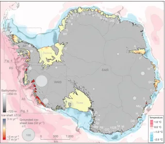
Figure 1.1: Seaward of the ice shelves, estimated average sea-floor potential temperatures (ino_C) from the World Ocean Circulation Experiment Southern Ocean Atlas (pink to blue) are overlaid on continental-shelf bathymetry (in metres) (greyscale, landward of the continental-shelf break). Grey labels indicate Antarctic Peninsula (AP), West and East Antarctic Ice Sheets (WAIS and EAIS), Bellingshausen Sea (BS), Amundsen Sea (AS) and the Ross and Ronne ice shelves. White labels indicate the ice shelves (clockwise from top) Vigridisen (V), Nivlisen (N), 17 East (17E), Borchgrevinkisen (B), 23 East (23E), 26 East (26E), Unnamed (U), Amery (A), Publications (P), West (W), Shackleton (SH), Conger (C), Totten (T), Moscow University (MU), Holmes (H), Dibble (DB), Mertz (M), Ninnis (NI), 152 East (152E), Cook (CO), Rennick (RE), Borchgrevink-Mariner (BM), Aviator (AV), Nansen (N), Drygalski (D), Filchner (F), Brunt (BR), Stancombe-Wills (S), Riiser-Larsen (R), Quar (Q), Ekstrom (E), Jelbart (J) and Fimble (FI). Ice shelves are coloured to show the thinning rate in metres/year. Grey circles show relative ice losses for ice-sheet drainage basins (outlined in grey) that lost mass between 1992 and 2006. Taken from Pritchardet al.(2012).

and high-resolution photography. These techniques typically provide data over a wide geographic extent and are crucial in understanding regional and temporal patterns. How-ever, they do not provide any insight into why these changes are occurring. Such insights require much more localised observations, capable of measuring or inferring properties near the ice-ocean interface.

(21)

Ice Sheet Ice Shelf

[image:21.595.160.503.102.340.2]

Grounding Line

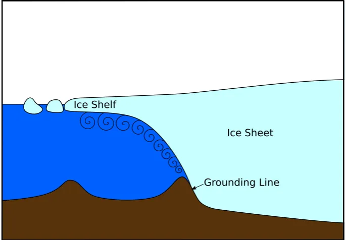
Figure 1.2: A schematic of a marine terminating glacier with a protruding ice shelf. The

ground-ing line is the location where the ice sheet becomes disconnected from the bedrock. A turbulent convective plume is seen rising up the underside of the ice shelf. The vertical scale has been exaggerated for ease of viewing.

can provide more detailed spatial information but are limited to one specific time. Such measurements are also restricted by how close ships can safely get to the ice face. In con-trast, moorings placed through drill holes can be placed closer to the ice-ocean interface and left in place for several years. They are however limited to providing spot measure-ments at a fixed location. As such arrays of moorings are often deployed to obtain more complete information about a specific glacier. All field investigations in Antarctica and Greenland are also faced with the challenges associated with operating in a remote and harsh environment. This increases the cost and limits the field season when instruments can be deployed.

Due to these challenges, oceanographic field observations, particularly near the ice-ocean interface, are sparse. Compounding the restrictions of limited data is the substantial uncertainty in the data produced by field investigations. Figure 1.3 shows a set of field observations of the mass loss from Antarctic ice shelves (Rignot & Jacobs, 2002) which demonstrate this large uncertainty.

Perhaps the observations made closest to the ice-ocean interface were made by an Autonomous Underwater Vehicle (AUV) that was deployed into the cavity beneath the Pine Island Glacier ice shelf (Jenkins et al., 2010a). The AUV measured profiles of po-tential temperature, salinity, dissolved oxygen concentration and light attenuation along a transect in the glacier flow direction as shown in figure 1.4.

(22)

Figure 1.3: Ice shelf dissolving velocities (m/yr) as a function of driving temperature difference (◦C) as measured by Rignot & Jacobs (2002).

make extrapolation to the more general problem of ice-ocean interactions difficult. The AUV only measured a single transect within one ice shelf cavity and it is possible that different conditions would be observed under different ice shelves or even in a different location under the Pine Island Glacier ice shelf. Longitudinal channelization in the ice shelf (Millgateet al., 2013) and the Coriolis force (Sternet al., 2014) could divert the flow of meltwater, while subglacial plumes could change the dynamics close to the ice (Straneo & Cenedese, 2015). All of these processes, among others, could affect the ocean properties across an ice shelf cavity.

The difficulties in obtaining extensive and accurate measurements around Greenland and Antarctica, in particular near the ice-ocean interface, create a need for other techniques to supplement field observations. Theoretical, numerical, and experimental studies all lead to a greater understanding of the important processes in this region and help to guide field observations to ensure that they are as effective as possible.

1.2 Theory relevant to ice-ocean interactions

1.2.1 Melting and dissolving

(23)

[image:23.595.219.445.101.705.2]

(24)

T_f T_i

T_s C_s

Cf

Salt water

x V

Ice

hC

[image:24.595.151.379.98.300.2]

h_T C_i

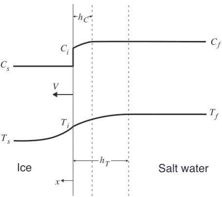
Figure 1.5: The compositional and thermal profiles when ice dissolves at a velocityV into salt

water of salinityCf and temperatureTf. The thermal boundary layer has a thicknesshT and the

compositional boundary layer has a thicknesshC. Taken from Kerr & McConnochie (2015).

the pressure dependent melting point. In contrast, when the ambient fluid is sufficiently cold (or salty), ice will dissolve. Dissolving is controlled both by heat and salt transfer and will result in the interface salinity being non-zero and the interface temperature be-ing below the pressure dependent meltbe-ing point (Woods, 1992; Kerr, 1994b). Figure 1.5 shows the salinity and temperature profiles that exist when ice dissolves at a velocity,

V. At oceanic salinities, ice will dissolve in temperatures less than around 6 o_{C (Kerr &}

McConnochie, 2015). As such, when considering the mass loss from the Antarctic and Greenland ice sheets one must consider the dissolving regime and hence, both the thermal and compositional boundary layers.

Throughout this thesis the process where ice either melts or dissolves is typically referred to using the more general term: ablation. This is done to avoid confusion with geophysical literature where the ablation of Antarctica and Greenland is often described as melting, despite dissolving being more accurate. Although the term ablation is used, all of the experiments presented in this thesis involved the dissolution of ice.

1.2.2 Plume theory

Ablation of ice into salt water releases cold and fresh meltwater which can form a posi-tively buoyant plume that quickly becomes turbulent and rises up the side of the ice face. Understanding the behaviour of this turbulent plume is crucial to understanding ice-ocean interactions as it links the warm and salty ocean waters with the ablating ice face.

(25)

into the plume at a given height, is proportional to some characteristic velocity at that height. This can be described mathematically as

ue=αw (1.1)

where ue is the entrainment velocity,α is the entrainment coefficient, and w is a

charac-teristic vertical plume velocity.

Plume models often make use of simplified ‘top-hat’ profiles (Morton et al., 1956). Top-hat profiles replace the physically realistic Gaussian velocity and buoyancy profiles with a step profile where the velocity and buoyancy are zero outside the plume and a constant value within the plume. This can be done in such a way that the volume flux, momentum flux and buoyancy flux are all conserved. When comparing entrainment coef-ficients, care must be taken to ensure that the same velocity scale is used as the value of the coefficient will differ depending on whether the maximum or top-hat plume velocity is used. Throughout this thesis, entrainment coefficients are typically quoted in terms of the maximum plume velocity, as this velocity can be directly measured in our experiments.

The entrainment assumption has been found to be robust across a variety of plumes with slightly different entrainment coefficients for different geometric configurations (e.g. Ellison & Turner, 1959; Grella & Faeth, 1975; Sangras et al., 1999). For conical plumes from a point source of buoyancy an entrainment coefficient of approximatelyα= 0.12 has been measured.

However, this value of the entrainment coefficient is unlikely to be appropriate when considering the plumes that form next to ice shelves and icebergs. The plumes resulting from the ablation of ice are best represented as two-dimensional planar plumes that have a distributed source of buoyancy up the ice face. The presence of a solid wall on one side of the plume is also likely to affect the entrainment coefficient and plume velocity. The plume that forms next to a dissolving ice wall will be discussed in more detail in chapters 3, 4 and 5.

1.2.3 Double-diffusive convection

Double-diffusive convection is a type of convection that has been observed in a wide variety of situations. Two density affecting components with different rates of diffusion are required (Turner & Stommel, 1964). The differential diffusion of these two components can destabilise an initially stable arrangement or vice versa. Although double-diffusion requires sufficient time for diffusive processes to occur, it has been shown to be important in a number of flows where molecular diffusion would typically be ignored (Schmitt, 1994).

(26)

[image:26.595.98.433.213.422.2]

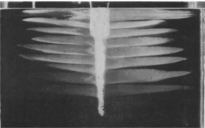
When ice ablates into a salinity gradient, such as is often the case in the ocean, the convective plume can intrude into the interior instead of rising to the surface (Huppert & Josberger, 1980; Huppert & Turner, 1980). This is a result of double-diffusion and is due to heat diffusing into the plume more rapidly than salt. The resulting flow can be seen in figure 1.6. Fluorescein dye has been frozen into the ice so that the meltwater can be tracked, showing a series of intruding layers on either side of the ice.

Figure 1.6: Ice ablating into a salinity gradient illuminated with fluorescein dye. Double-diffusive

layers are shown by the dye intruding into the interior. Taken from Huppert & Turner (1980).

Both Huppert & Turner (1980) and Huppert & Josberger (1980) measured the double-diffusive layer thickness in a given salinity gradient. The layer height, h, was found to be given by:

h= 0.65[ρ(Tw, Cf)−ρ(Tf, Cf)]

dρ

dz

−1

(1.2)

and

h= 0.65[ρ(Tf p, Cf)−ρ(Tf, Cf)]

dρ

dz

−1

(1.3)

respectively, where ρ(T, C) is the fluid density at temperature T and salinityC, dρ/dz is the vertical density gradient, subscript w relates to the rising plume, subscript f relates to the far-field and subscript f prelates to the freezing point at the mean far field salinity.

(27)

small (<10%).

1.3 Idealized studies of ice-ocean interactions

Given the difficulty in making reliable observations close to the ice-ocean interface (see section 1.1), idealized modelling studies are frequently used to gain additional insight. In the following section these have been separated into theoretical, experimental, and numerical models. Despite this separation, many studies involve components of two or three of the separate categories. These different components will be described separately in the following sections.

1.3.1 Theoretical models

One of the earliest models examining ice-ocean interactions was developed by Josberger & Martin (1981) to describe their experimental results. Three distinct flow regimes were described depending on the far-field temperature and salinity. When the far-field temper-ature and salinity lie between the line of maximum density and the freezing point, the flow will be purely upward. As the far-field temperature and salinity increase beyond the line of maximum density, a bidirectional flow begins to exist in the laminar section of the flow. This is caused by the different thicknesses of the thermal and salinity boundary layers (figure 1.5) and their opposing buoyancies. After the initial laminar section, the thermal and compositional buoyancies become well mixed within the turbulent plume and the flow becomes purely upwards. If the far-field temperature is increased further, or the far-field salinity is reduced, the flow becomes purely downward as the thermal buoyancy begins to dominate the compositional buoyancy. The second regime is the most relevant to ice-ocean interactions in the polar regions. However, due to the long length scales, the laminar section at the base of the ice shelf is generally unimportant and a purely upward flow would be expected for almost the entire height of an ice shelf or iceberg.

Wells & Worster (2008) presented a model that described the convective plume that forms next to an isothermal surface. They describe a convective plume with a turbulent outer section and laminar near-wall region. There is a transition that occurs after a sufficient height where the inner layer stops being driven by its own buoyancy and is instead driven by the shear imposed on it from the outer turbulent layer. In the shear driven regime a higher rate of heat transfer is predicted.

(28)

Wells & Worster (2011) developed a theoretical model that describes the ablation of a vertical solid into a two-component fluid such as cold salty water. The melting and dissolving of a solid are considered separately. The boundary layer structure is predicted for both dissolving and melting as well as the transition between the two regimes. Un-fortunately, the model is limited to the region where the resulting convection is laminar. At oceanic salinities this corresponds to approximately 10-20 cm. As such the model is of limited use when considering ice shelves or icebergs on a geophysical scale, which typically have heights on the order of 102₋₁₀3 _m.

Magorrian & Wells (2016) extended the analysis of Wells & Worster (2008) to include a stratified water column and a sloping ice face. It was assumed that on geophysical scales the inner layer is driven by shear and not its own buoyancy. Similarly to the experiments conducted by Huppert & Turner (1980) and Huppert & Josberger (1980), a series of intruding layers were predicted. However, instead of these layers being caused by double diffusion they are due to the plume moving above the location of neutral buoyancy and then decelerating. The predicted layer thickness and melt rate are both sensitive to the slope of the ice face with different dependencies for small and large slopes.

1.3.2 Laboratory expriments

Laboratory experiments have previously been utilised to examine the problem of ice-ocean interactions (e.g. Huppert & Josberger, 1980; Huppert & Turner, 1980; Josberger & Mar-tin, 1981). The most significant limitation that is common to all laboratory experiments has been the physical scale on which experiments can be conducted. The first challenge for laboratory experiments has been achieving sufficient height for the resulting flow to be predominantly turbulent. However, even once this is satisfied there remains a significant difference between laboratory and geophysical scales. In particular this leaves potential transitions such as that described by Wells & Worster (2008) untested. Theoretically this could be overcome with suitable scaling but in practice such scaling has not been convincingly developed.

(29)

Josberger & Martin (1981) conducted a careful series of experiments in which a 1.2 m high vertical ice wall was exposed to homogeneous salty water. These experiments are particularly relevant to icebergs and ice shelves as there were several experiments con-ducted at low temperatures. The ablation rate at temperatures below 9 o_{C is described}

by

M = 0.76T

1.6

d

z1/4 (1.4)

where M is the ablation rate in µm/s, Td is the driving temperature, defined as the

difference between the far-field temperature and the freezing point at the far-field salinity, and z is the height up the ice wall in mm. Between 9o_{C and 20} o_{C the ablation rate is}

instead given by

M = 3.55Td−5.89

z1/4 . (1.5)

This change in behaviour reflects the transition from dissolving to melting. When the ice is dissolving, increasing the far-field temperature will cause the interface salinity to decrease and hence, the buoyancy to increase. When the ice is melting, the interface salinity is zero and the buoyancy will be unaffected by rising far-field temperatures, leading to a linear dependence of M on Td. These experiments will be discussed more fully and compared

with our own in Chapter 2.

More recently, Sciasciaet al.(2014) conducted laboratory experiments aimed at repli-cating the conditions found in the glacial fjords that surround Greenland. The experiments examined the circulation that could be driven by changes in density at the mouth of the fjord. A two-layer fluid was considered and it was found that density changes at the fjord mouth can propagate up the fjord to alter the ablation rate at the ice ocean interface. This study highlights the sensitivity of ice-ocean processes to external flows and small anomalies in the temperature and salinity of the ocean.

Further experiments using a similar apparatus explored the effect of two interacting freshwater plumes that were released at the base of a vertical ice face (Cenedese & Gatto, 2016). These experiments investigated the effect of freshwater plumes such as have been observed near the fronts of Greenland ice shelves (Straneo & Cenedese, 2015). A strong link between the area of the plume in contact with the ice face and the integrated ablation rate was found.

Both of these recent laboratory studies were limited to a vertical scale of 0.3 m (Sciascia

et al., 2014; Cenedese & Gatto, 2016). In the experiments performed by Sciascia et al.

(30)

1.3.3 Idealized numerical modelling

More recently, direct numerical simulations have been performed that resolve the turbulent boundary layer and laminar sublayer (Gayen et al., 2015, 2016). Resolving the ice-ocean interactions is computationally expensive and limits the scale of these simulations to a comparable height to that which can be achieved with laboratory experiments.

Results from recent direct numerical simulations (Gayen et al., 2016) agree strongly with the laboratory results that are presented in chapters 2 and 3. In addition to the ablation velocity and interface temperature that are measured experimentally, turbulent quantities such as the dissipation rate and the shear production rate are computed. It is found that over a 1 m simulation height, the turbulent kinetic energy transitions from being produced almost entirely from convective instabilities to being supplied at compa-rable rates by convective instabilities and by shear production. It is noted that, despite similarities, this is not the same transition that was described by Wells & Worster (2008). The ability to compute turbulent statistics, that are difficult to measure experimentally, is an advantage of direct numerical simulation over laboratory experiments. However, the computational cost limits the scope of studies relying on direct numerical simulations. Direct numerical simulations will continue to be important tools in the investigation of ice-ocean interactions, especially as computational power increases.

1.4 Large-scale numerical studies

Idealized models such as were discussed in section 1.3 provide useful insight into the physi-cal processes occuring at the ice-ocean interface. However, extending them to a geophysiphysi-cal scale so that the results can be compared to field observations is often challenging. The studies described in section 1.3 had a maximum length scale of 1.2 m whereas the ice shelves around Antarctica and Greenland are frequently many hundreds of metres high. To bridge the gap between small-scale idealized studies and large-scale ice shelves, numeri-cal models are typinumeri-cally used. In order to simulate realistic geometry, small-snumeri-cale processes need to be parameterized (e.g. Xuet al., 2013; Carrollet al., 2015; Slateret al., 2015).

The thermodynamic processes that occur at the ice-ocean interface are almost univer-sally parameterized by the so-called three equation model (Jenkins, 1991, 2011; Holland

et al., 2008). The ablation rate and the interface conditions are given by the following three equations:

˙

mL+ ˙mci(Tb−Ti) =cC_d1/2UΓT(T −Tb) (1.6)

˙

m(Sb−Si) =C_d1/2UΓS(S−Sb) (1.7)

Tb =λ1Sb+λ2+λ3zb (1.8)

where ˙m is the ablation rate, L is the latent heat of fusion, ci the specific heat capacity

of ice, T is the temperature, c is the specific heat capacity of the fluid, Cd is the drag

(31)

coefficients,Sis the salinity,λ1,λ2andλ3are constants that define the pressure dependent

liquidus equation, subscript irefers to ice properties, and subscript b refers to properties at the ice-ocean interface. No subscript refers to properties in the buoyant meltwater plume which are assumed to be constant across the plume. It is generally assumed that the ice-ocean interface is a non-moving boundary for simplicity.

Equations 1.6 and 1.7 can be rewritten to explicitly give the ablation rate and interface temperature:

˙

m=C_d1/2UΓS

S₋Sb Sb−Si

(1.9)

(T ₋Tb) =

ΓS

ΓT

L+ci(Tb−Ti) c

S−Sb Sb−Si

(1.10)

and solved using equation 1.8 to link the interface temperature and interface salinity. Typical values of the drag coefficient,Cd, and the two transfer coefficients, ΓT and ΓS,

areCd= 2.5×10−3, ΓT = 2.2×10−2 and ΓS= 6.2×10−4 (Jenkins, 2011). This leads to

constant thermal and haline Stanton numbers given byStT ,S =C

1/2

d ΓT,S of 1.1×10−3 and

3.1×10−5_{, respectively. In original iterations of the three-equation model (e.g. Jenkins,}

1991) a more complex formulation of the turbulent transfer coefficients was used based on laboratory experiments examing the turbulent boundary layers next to hydraulically smooth surfaces (Kader & Yaglom, 1972, 1977). These more complex formulations involved an empirical dependence on the Reynolds and Prandtl numbers. Geophysical observations under sea ice have suggested that including a dependence on the Reynolds and Prandtl numbers does not improve model predictions (McPhee, 1992; McPhee et al., 1999). As such, the simpler parameterization given in equations 1.6 and 1.7 has typically be used in recent studies.

Observations under sea ice (McPhee, 1992; McPheeet al., 1999) and near horizontal ice shelves (Jenkins et al., 2010b) have been used to evaluate the coefficients in equations 1.6 and 1.7. However, it has not been possible to validate the functional form of the parame-terization. Furthermore, it is not clear that the transport of heat and salt to the ice-ocean interface will be the same under sea ice as next to ice shelves. The underside of sea ice is often horizontal and rough. In contrast, ice shelves and the fronts of tidewater glaciers are much smoother and sloping or near vertical. These differences could lead to significantly altered dynamics. Specifically, convection is expected to be much less important under sea ice. This uncertainty means that the results of simulations employing the three-equation model should be viewed somewhat cautiously until the transfer parameterizations can be more thoroughly validated (Straneo & Cenedese, 2015).

1.4.1 Results derived from the three-equation model

(32)

applicable to the laboratory experiments discussed in later chapters.

Kusahara & Hasumi (2013) have simulated the entire Antarctic ice sheet using a cou-pled sea ice-ocean model (COCO) with ice shelves included and the three-equation model to parameterize ice-ocean interactions. Under current climate conditions, the basal mass loss from Antarctic glaciers is estimated to be 770–944 Gt/yr. This is compared to several previous estimates derived from observational and modelling studies of 400–1000 Gt/yr and 756–1600 Gt/yr respectively. The sensitivity of this estimate was tested in two cli-mate perturbations: strengthened westerly winds and increased surface air temperatures. The simulated basal mass loss is found to be almost insensitive to changes in the westerly winds but strongly dependent on the surface air temperature.

An earlier form of the three-equation model proposed a parameterization of ice-ocean interactions that was velocity independent (Hellmer & Olbers, 1989). Dansereau et al.

(2013) compared results derived from the velocity dependent and velocity independent versions of the parameterization. Both an idealized and a realistic geometry were tested with the realistic geometry representing the Pine Island Glacier ice shelf. Although the total ablation rate is relatively insensitive to which parameterization is used, the spatial distribution of ablation is significantly altered. When the velocity independent param-eterization is used, the location where the meltwater plume exits the ice shelf cavity is associated with low ablation rates due to the plume being cooler. In contrast, the velocity dependent parameterization leads to high ablation rates where the plume exits the cavity due to the plume being at a maximum velocity.

A similar result was found by Sciascia et al. (2013) for an East Greenland fjord. A velocity independent parameterization resulted in an ablation rate that was uniform with depth for most of the water column. This contrasts with a velocity dependent parameter-ization where the ablation rate increases over the bottom 300 m of the water column as the meltwater plume accelerates.

Schodlok et al.(2016) implemented the three-equation parameterization into circum-polar simulations of the Antarctica. The effect of vertical resolution is investigated by conducting simulations with both 50 and 100 vertical levels. Use of 100 vertical levels gave a vertical resolution finer than 30 m within the ice shelf cavity. Simulations with 50 vertical levels dramatically overestimated the ablation rate compared to observations (e.g. simulated ablation rates of 534±40 Gt/yr compared with observations of 41.9±10 Gt/yr at the Filchner Ice Shelf). Once the vertical resolution was increased, the simulated ablation rate was closer to the observed value (48.6_±4.7 Gt/yr for the Filchner Ice Shelf) but typ-ically remained larger. This dramatic change was associated with a better representation of the meltwater plume in the high resolution simulations.

(33)

of these processes and numerous studies investigating them.

Most of these studies (e.g. Xu et al., 2012, 2013; Sciascia et al., 2013; Carroll et al., 2015) use the iteration of the three-equation model presented in Jenkins (2011). These studies typically find that the local ablation rate scales like Q1s/3 and linearly with Td,

whereQs is the subglacial volume flux and Tdis the driving temperature of the ocean.

1.5 Thesis Outline

Given the difficulty in obtaining field observations in the polar regions and the uncertainty regarding the applicability of numerical ice-ocean parameterizations, a deeper understand-ing of the small-scale physical processes that control the ice-ocean interface is needed. This understanding will help to inform the development of numerical parameterizations and serve as a currently unavailable test of their validity. In turn, this will help guide future field observations to ensure that they are as effective as possible.

This thesis presents laboratory experiments that aim to explore the ablation of a vertical ice wall in several situations. It is hoped that these experiments will improve the understanding of physical processes relevant to ice-ocean interactions and how they may influence the future of Antarctica and Greenland.

Chapter 2 (Kerr & McConnochie, 2015) presents experiments focused on a vertical ice wall dissolving into an ambient fluid of uniform properties. The ablation velocity and interface temperature of the ice are measured and the results are compared with previous experimental data (Josberger & Martin, 1981). The experiments were designed to test a theoretical model that is also presented in this chapter. This model accurately predicts the ablation velocity and interface conditions of a dissolving ice wall, based on the ambient fluid temperature and salinity.

Chapter 3 (McConnochie & Kerr, 2016a) extends the experimental results presented in chapter 2 by focusing on the turbulent plume that forms next to a dissolving ice face. As ice dissolves, relatively fresh water is produced which rises next to the ice as a turbulent wall plume. This plume plays an important role in transporting heat and salt to the ice face and maintaining ablation of the ice. A previous model of this wall plume (Cooper & Hunt, 2010) is extended based on the experimental results and applied to a typical Antarctic iceberg.

As previously noted, stratification can have significant impacts on ice-ocean interac-tions (see section 1.2.3). In chapter 4 (McConnochie & Kerr, 2016b), the effect of strat-ification is investigated. The experimental results are compared to the much larger but more weakly stratified geophysical scale through a non-dimensional stratification param-eter based on the model of a turbulent wall plume presented in chapter 3.

(34)

laboratory experiments are used to investigate this enhanced mass loss and to observe how the wall plume and interface temperature are altered by the presence of a subglacial discharge.

(35)

Chapter 2

Dissolution of a vertical solid

surface by turbulent compositional

convection

Abstract

We examine the dissolution of a vertical solid surface in the case where the heat and mass transfer is driven by turbulent compositional convection. A theoretical model of the turbulent dissolution of a vertical wall is devel-oped, which builds on the scaling analysis presented by Kerr (1994b) for the turbulent dissolution of a horizontal floor or roof. The model has no free pa-rameters and no dependence on height. The analysis is tested by comparing it with laboratory measurements of the ablation of a vertical ice wall in contact with salty water. The model is found to accurately predict the dissolution ve-locity for water temperatures up to about 5–6◦C, where there is a transition from turbulent dissolution to turbulent melting. We quantify the turbulent convective dissolution of vertical ice bodies in the polar oceans, and compare our results with some field observations.

2.1 Introduction

Over the past decade, an important component of global climate change has been the increasingly rapid decrease in the mass of the Antarctic and Greenland Ice Sheets (Rignot

et al., 2011). This ongoing mass loss is occurring on the underside and fronts of ice shelves formed where glaciers reach the polar oceans (Jenkinset al., 2010a) and from the icebergs that calve from them (Buddet al., 1980). Around Antarctica, Rignotet al.(2013) estimate that about 55% of the annual mass loss (1500 Gt/year) is from ice shelves and about 45% (1265 Gt/year) is from calved icebergs. Field observations of both icebergs and ice shelves indicate that this mass loss is an increasing function of ocean temperature (e.g. Budd

et al., 1980; Shepherdet al., 2004).

(36)

salinity is zero, and the interface temperature is the melting point of ice (e.g. 0 ◦C at atmospheric pressure). In contrast, dissolving will occur when the sea is close to or below the melting point of ice, and it is controlled by a combination of heat and mass transfer (Woods, 1992; Kerr, 1994b). During dissolving, the interface salinity is non-zero, and the interface temperature is less than the melting point of ice.

In a recent study, Wells & Worster (2011) quantified the melting and dissolving of a vertical solid surface driven by laminar compositional convection. They analysed the structure of the thermal and compositional boundary layers during both melting and dis-solving, and determined the condition for the transition between the melting and dissolving regimes. However, this analysis cannot be used to predict the melting and dissolving of large bodies of ice in the polar oceans, because the convective flow becomes turbulent after a vertical distance of 10–20 cm (Josberger & Martin, 1981; Carey & Gebhart, 1982; Johnson & Mollendorf, 1984), while icebergs have vertical heights of 100 m in the North Atlantic Ocean and 250 m in the Southern Ocean.

In this paper, we aim to quantify the turbulent dissolution of a vertical ice wall. In section 2.2, we present a theoretical model of dissolution by turbulent compositional con-vection of a vertical solid surface. In section 2.3, the model is compared with experimental observations of vertical ice walls ablating in water at oceanic salinities, made by Josberger & Martin (1981) and by ourselves. In section 2.4, we quantify the turbulent convective dissolution of vertical ice bodies in the polar oceans. Our conclusions are given in sec-tion 2.5.

2.2 Dissolving theory

In this section, we examine turbulent thermal convection on vertical and horizontal bound-aries in section 2.2.1, before the dissolution of a vertical solid surface by turbulent com-positional convection is considered in section 2.2.2.

2.2.1 Turbulent thermal convection

In understanding mass transfer due to turbulent compositional convection, very useful insight can be gained by examining the experimental measurements on turbulent heat transfer by natural convection tabulated by Holman (2010).

For turbulent natural convection on an isothermal vertical boundary of temperature

Tw, the expression for the Nusselt number N u at high Rayleigh numbersRa is given by

N u= 0.10Ra1/3, (2.1)

(Holman, 2010, p. 335), where N u = qH(k(Tw −Tf))−1, q is the heat flux from the

boundary, H is the height of the boundary,k is the thermal conductivity of the fluid,Tf

is the far-field temperature of the fluid,Ra=gα(Tw−Tf)H3(κν)−1,gis the gravitational

(37)

of the fluid, andνis the kinematic viscosity of the fluid. Equation 2.1 was measured in air by Warner & Arpaci (1968) using a 3.7 m high plate, for Rayleigh numbers that ranged from 109 _{up to 10}12_.

For turbulent natural convection on a constant-heat-flux vertical boundary, the Nusselt number at high flux Rayleigh numbers Raf is given by

N u= 0.17Ra1_f/4, (2.2)

(Holman, 2010, p. 336), where Raf =gαqH4(kκν)−1. Equation 2.2 was measured in air

by Vliet & Ross (1975) using a 7.3 m high plate, for flux Rayleigh numbers that ranged from 2×1013 _{up to 10}16_{. Since}_Ra

f =Ra N u, we note that equation 2.2 is equivalent to

N u= (0.17)4/3Ra1/3 = 0.094Ra1/3, (2.3)

for Rayleigh numbers that range from 5×1010 _{to 6}_×₁₀12_{, which demonstrates that the}

turbulent heat transfer expressions 2.1 and 2.2 are in very good agreement.

For turbulent natural convection from a horizontal boundary, the Nusselt number at high Rayleigh numbers is given by

N u= 0.156Ra1/3, (2.4)

where H here is the height of the fluid layer. Equation 2.4 was measured in 0.45 m high water by Katsaroset al. (1977), for Rayleigh numbers of 3_×108 _{– 4}_×₁₀9_.

It is important to note that equations 2.1, 2.3 and 2.4 show that a one-third power law dependence on Rayleigh number applies equally as well for turbulent natural convection at both horizontal and vertical boundaries. For a horizontal boundary, the one-third power law dependence implies that the turbulent heat flux is independent of the height of the fluid (cf. Turner, 1973, p. 213). For a vertical boundary, the one-third power law dependence implies that the turbulent heat flux is independent of the height of the boundary and independent of position on the vertical boundary(cf. Holman, 2010, p. 337).

2.2.2 Dissolution of a vertical solid surface by turbulent compositional convection

Consider the turbulent dissolution at velocityV of a vertical solid surface of composition

Cs, melting temperature Tm and far-field temperatureTs, in contact with a semi-infinite

fluid with a far-field compositionCf and a far-field temperatureTf. The resulting thermal

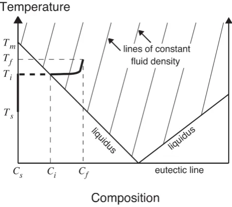
and compositional profiles are shown in figure 2.1 (cf. figure 1(b) of Wells & Worster, 2011) and illustrated on a typical phase diagram in figure 2.2. At the interface between the solid and the fluid, the temperatureTi and compositionCi are constrained thermodynamically

to lie on the liquidus curve

(38)

T_f T_i

T_s C_s

C_f

Salt water

x V

Ice

h_C

[image:38.595.145.386.96.314.2]

h_T C_i

Figure 2.1: The thermal and compositional profiles when ice dissolves into salt water at velocity

V. The thermal boundary layer has a thickness hT and the compositional boundary layer has a

thicknesshC.

Figure 2.2: The path on a simple phase diagram of the thermal and compositional profiles shown

in figure 2.1. The dotted portion of the path represents the jump in composition at the dissolving interface.

which gives the freezing temperature of the fluid as a function of concentration. Within the solid, the balance between thermal diffusion and ablation results in a temperature given by

T(x) =Ts+ (Ti−Ts)e−x/hs (2.6)

(Carslaw & Jaeger, 1986), where the length scale hs = κs/V, and κs is the thermal

diffusivity of the solid.

[image:38.595.145.384.377.590.2]

(39)

interface. If the respective turbulent fluxes to the interface through these layers are FC

and FT, the effective layer thicknesses hC and hT can be defined by

FC =

D(Cf −Ci) hC

(2.7)

and

FT =

kf(Tf−Ti) hT

, (2.8)

where D and kf are the compositional diffusivity and thermal conductivity of the fluid.

For simplicity, we neglect the volume change associated with the phase change (cf. Woods, 1992), which for ice is about 8%. The boundary layer fluxes are linked to the dissolving velocity V by the interfacial conditions

FC =V(Ci−Cs) (2.9)

and

FT =V(ρsLs+ρscs(Ti−Ts)), (2.10)

whereρs,Lsandcsare the density, latent heat and specific heat of the solid. Equations 2.9

and 2.10 represent conservation of composition and conservation of heat at the interface.

The interface between the solid and the fluid is assumed to be flat, and the composi-tional buoyancy released at the interface is assumed to dominate the thermal buoyancy, i.e. that the ratio_Rof these buoyancies satisfies the condition

R ≡ _α_[_ρ β(Cf −Cs)

sLs+ρscs(Ti−Ts)]/ρfcf

1, (2.11)

where α is the coefficient of thermal expansion andβ is the equivalent coefficient for the variation of density with composition (cf. Kerr, 1994a,b).

Following Kerr (1994b), it is envisaged both the compositional and thermal boundary layers grow diffusively with time t:

hC ∼ √

Dt (2.12)

and

hT ∼

p

κft, (2.13)

where cf and κf ≡ kf/ρfcf are the specific heat and thermal diffusivity of the fluid,

until a typical time τ when they are periodically removed by the eddies associated with the turbulent buoyant compositional convection (cf. Lick, 1965; Howard, 1966). From the empirical expressions 2.1 and 2.3 for turbulent heat transfer from a vertical boundary given in section 2.2.1, the mass transfer due to turbulent compositional convection is expected to be given by

N u=γ Ra1/3, (2.14)

(40)

compositional boundary layer thickness

hC =

1

γ

Dµ g(ρf −ρi)

1/3

, (2.15)

where g is the acceleration due to gravity, ρf is the density of the far-field fluid, ρi is the

density of the fluid at the interface, andµis the fluid viscosity. Combining equations 2.15, 2.12 and 2.13 gives

hT =hC

κ_f

D

1/2

= 1

γ

µ2κ3_f

Dg2₍_ρ

f −ρi)2

!1/6

(2.16)

and

τ _≈ 1 γ2

µ2 Dg2₍_ρ

f −ρi)2

1/3

. (2.17)

Substitution of equations 2.7 and 2.15 into equation 2.9 then yields the prediction that the dissolving velocity

V =γ

g(ρf−ρi)D2 µ

1/3

Cf −Ci Ci−Cs

, (2.18)

while combining equations 2.5, 2.8, 2.10, 2.16 and 2.18 shows that

Tf−TL(Ci) =

ρsLs+ρscs(TL(Ci)−Ts) ρfcf

D κf

1/2

Cf −Ci Ci−Cs

. (2.19)

In the above analysis, it has been implicitly assumed that the distance√Dτ over which compositional diffusion occurs is large in comparison with the distance V τ that the solid has dissolved in the convective timescaleτ. From equations 2.15, 2.17 and 2.18, it is found that

V τ ≈ hC

C , (2.20)

where

C ≡ Ci−Cs

Cf −Ci

. (2.21)

Equations 2.18 and 2.19 are therefore asymptotically correct when C 1. However, ifC

is smaller (i.e. _{C ∼} 1), then equation 2.20 suggests that hC is more accurately estimated

by

hC = √

Dτ+V τ = 1

γ

Dµ g(ρf −ρi)

1/3

1 +1

C

, (2.22)

which results inV and Tf −Ti being given by

V =γ

g(ρf −ρi)D2 µ

1/3

Cf −Ci Cf −Cs

(41)

and

Tf−TL(Ci) =

ρsLs+ρscs(TL(Ci)−Ts) ρfcf

D κf

1/2

Cf −Ci Cf −Cs

. (2.24)

It is then concluded that the dissolving rate is given by equation 2.23, once Ci is

evalu-ated from equation 2.24. We also note that when when _C 1, √Dτ V τ, and the above scaling analysis breaks down, as the turbulent dissolving undergoes a transition to turbulent melting (see the appendix of Kerr, 1994b).

2.3 Comparison with laboratory experiments

[image:41.595.219.444.301.602.2]

2.3.1 The experiments of Josberger & Martin (1981)

Figure 2.3: Sketch by Josberger & Martin (1981) of the convective flows beside the ice wall, for

Tf <20◦C andCf = 2.90–3.52 wt% NaCl.

Josberger & Martin (1981) conducted a careful series of experiments in which a vertical ice wall ablated in contact with homogeneous aqueous solutions of sodium chloride. The ice was bubble-free, up to 1.2 m high, and had an initial temperature of−1◦C. The solutions had compositionsCf from 2.90 to 3.52 wt% NaCl, and temperaturesTf that ranged from

0 to 27 ◦_{C. For solution temperatures up to 20} ◦_{C, the convective flow on the lower part}

(42)

and its outer edge was seen to fluctuate with the passage of turbulent eddies.

The turbulent flow data from the 9 experiments of Josberger & Martin (1981) are summarized in table 2.1. The table lists the temperature Tf and composition Cf of

the sodium chloride solutions, the measured interface temperature Tw, and the ablation

velocities V measured at various vertical distances z above the height on the ice wall at which the upward flow became turbulent. The interface temperatures were found to be constant to within 0.02 ◦_{C along the ice in each experiment. The ablation velocities}

are also reasonably constant, to within about 5–10%. We note that Josberger & Martin (1981) attempted to understand their ablation results using a V ∝z−1/4 power law, but this scaling law does not fit all their data well (i.e. it gives a variation with z of 23% for experiment 4, and a variation of 20% for experiment 5; see their table 3), and it should only be relevant to ablation by laminar flow (see Wells & Worster, 2011).

When the turbulent dissolution model in section 2.2.2 is compared with the turbulent ablation experiments of Josberger & Martin (1981), it can only be applied to experiments 1–6, as these are the only experiments that are in the dissolving regime. The turbulent flow in these experiments covers vertical length scales of about 0.1–1 m, and Rayleigh numbers of about 1010_–1014_{. The corresponding model predictions are listed in table 2.2. The}

predicted interface temperatures Ti, which are determined from equations 2.5 and 2.24,

agree with the measured interface temperaturesTw of Josberger & Martin (1981) to within

0.1 ◦_{C (see figure 2.4). We note that equation 2.24 is only expected to be accurate for}

C ∼1 or greater, butC is only 0.38 in experiment 6.

In figure 2.5, the measured dissolving velocities V of Josberger & Martin (1981) are plotted against the predicted velocity scale

V =

g(ρf −ρi)D2 µf

1/3

Cf −Ci Cf −Cs

(2.25)

from equation 2.23. The dissolving velocities are seen to lie on a straight line, whose slope

γ = 0.093_±0.010 is consistent with the value of about 0.097_±0.010 predicted from the turbulent heat transfer expressions 2.1 and 2.3 in section 2.2.1.

In experiments 7 to 9 of Josberger & Martin (1981), the fluid temperature Tf is too

high to allow a solution forCi in equation 2.24. Experiment 7 lies in the transition regime

between dissolution and melting (cf. the appendix to Kerr, 1994b), while in experiments 8 and 9, the interface temperatures are so close to 0 ◦C (see table 2.1) that these two experiments can be viewed as being in the regime of turbulent melting (cf. Kerr, 1994a; Josberger & Martin, 1981).

2.3.2 Our experiments

(43)

Experiment Tf Cf Tw z V

number (◦_C) _(wt%) ₍◦_C) _(mm) ₍_µ_m_/_s)

[image:43.595.206.458.100.364.2]

1 ₋0.10 2.99 ₋1.27 360 0.58 2 1.55 2.90 ₋0.92 70 1.22 200 1.02 3 2.00 3.00 ₋0.76 510 1.57 610 1.56 940 1.40 4 2.20 3.00 ₋0.76 115 1.87 250 1.89 5 2.66 3.44 −0.74 180 2.15 330 2.33 6 3.42 3.00 ₋0.59 470 2.47 520 2.23 7 6.85 3.395 ₋0.20 220 6.29 360 5.99 8 10.85 3.41 −0.06 240 9.58 370 9.16 9 16.31 3.52 ₋0.02 290 14.27

Table 2.1: The turbulent ablation results of Josberger & Martin (1981) and Josberger (1979). We

note thatTwfor experiment 7 is taken from Josberger (1979), as it is incorrectly given in Josberger

& Martin (1981).

Quantity 1 2 3 4 5 6 Units

Tf −0.10 1.55 2.00 2.20 2.66 3.42 ◦C

Cf 2.99 2.90 3.00 3.00 3.44 3.00 wt%

ρf 1022.7 1021.9 1022.6 1022.6 1025.9 1022.6 kg/m3

cf 4.03 4.04 4.03 4.03 4.01 4.03 J/g/◦C

kf 0.554 0.557 0.557 0.557 0.557 0.559 W/m/◦C

ν 1.85 1.83 1.82 1.82 1.82 1.80 mm2_/s

Ci 2.28 1.56 1.41 1.32 1.25 0.82 wt%

Ti -1.36 -0.92 -0.83 -0.79 -0.74 -0.48 ◦C ρi 1017.3 1011.7 1010.6 1009.9 1009.4 1006.0 kg/m3

C 3.22 1.16 0.89 0.79 0.58 0.38

V 5.6 13.7 16.7 17.9 22.2 25.7 µm/s

Table 2.2: Experimental parameters (ρf,cf,kf,µ) and theoretical predictions (Ci,Ti,ρi,C,V)

for experiments 1 to 6 of Josberger & Martin (1981) listed in table 2.1. The physical properties of the aqueous NaCl solutions were obtained from data in Washburn (1926), Weast (1989) and Batchelor (1967). Other parameters used areρsLs= 306 J/cm3 (Washburn, 1926),ρscs= 1.832

J/cm3_/◦_{C (Weast, 1989), and the expression} _D_{= 10}−5.144+0.0127Ti _cm2_{/s, where} _T

i has units of

◦_{C , which was inferred from data in Washburn (1926) that is accurate to about 3%. Consistent}

with the compositional and thermal profiles sketched in figure 2.1, the parameterν is evaluated at (Cf+Ci)/2 andTi, whilekf is evaluated atCf and (Ti+Tf)/2.

(44)

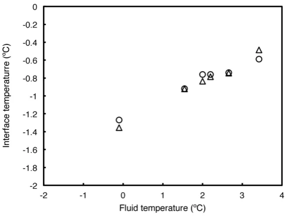
Figure 2.4: A comparison of the predicted interface temperatureTi(4) with the measured

[image:44.595.123.406.105.319.2]

inter-face temperatureTw() of Josberger & Martin (1981), plotted as a function of the temperature Tf of the NaCl solution. The experiments have a range inCf, from 2.90 to 3.44 wt% NaCl.

Figure 2.5: The dissolving velocities V of Josberger & Martin (1981), in comparison with the

velocity scale V defined by equation 2.25. The values lie on a straight line with a constant of proportionality of 0.093_±0.010.

that was 1.2 m high, 0.2 m wide and 1.5 m long. To limit heat transfer, the sidewalls of the tank consisted of an inner sheet of 20 mm thick acrylic and an outer sheet of 2 mm thick acrylic, separated by an 18 mm gap filled with argon gas. One endwall of the tank consisted of an aluminium heat exchanger, through which ethanol was circulated from a Julabo FP50 Refrigerated-Heating Circulator.

(45)

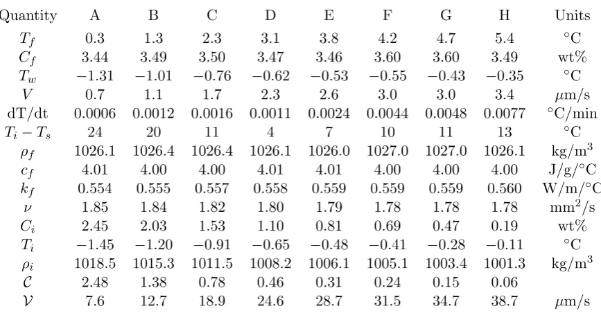
Quantity A B C D E F G H Units

Tf 0.3 1.3 2.3 3.1 3.8 4.2 4.7 5.4 ◦C

Cf 3.44 3.49 3.50 3.47 3.46 3.60 3.60 3.49 wt%

Tw −1.31 −1.01 −0.76 −0.62 −0.53 −0.55 −0.43 −0.35 ◦C

V 0.7 1.1 1.7 2.3 2.6 3.0 3.0 3.4 µm/s

dT/dt 0.0006 0.0012 0.0016 0.0011 0.0024 0.0044 0.0048 0.0077 ◦C/min

Ti−Ts 24 20 11 4 7 10 11 13 ◦C

ρf 1026.1 1026.4 1026.4 1026.1 1026.0 1027.0 1027.0 1026.1 kg/m3

cf 4.01 4.00 4.00 4.01 4.01 4.00 4.00 4.00 J/g/◦C

kf 0.554 0.555 0.557 0.558 0.559 0.559 0.559 0.560 W/m/◦C

ν 1.85 1.84 1.82 1.80 1.79 1.78 1.78 1.78 mm2_/s

Ci 2.45 2.03 1.53 1.10 0.81 0.69 0.47 0.19 wt%

Ti −1.45 −1.20 −0.91 −0.65 −0.48 −0.41 −0.28 −0.11 ◦C ρi 1018.5 1015.3 1011.5 1008.2 1006.1 1005.1 1003.4 1001.3 kg/m3

C 2.48 1.38 0.78 0.46 0.31 0.24 0.15 0.06

[image:45.595.126.560.98.324.2]

V 7.6 12.7 18.9 24.6 28.7 31.5 34.7 38.7 µm/s

Table 2.3: Experimental parameters, and theoretical predictions (Ci, Ti,ρi, C, V), for our 8 ice

ablation experiments (A–H). The physical properties of the aqueous NaCl solutions were calculated as described in table 2.2. Other parameters used areρsLs= 306 J/cm3(Washburn, 1926),ρscs=

1.832 J/cm3_/◦_{C (Weast, 1989), and the expression} _D _{= 10}−5.144+0.0127Ti _cm2_{/s, where} _T i has

units of ◦_{C , which was inferred from data in Washburn (1926) that is accurate to about 3%.} From the measured temperature rise dT/dt in the ice near the interface, equation 2.26 was used to evaluate the equivalent temperature differenceTi−Ts of a semi-infinite block of ice.

Once the ice wall was about 8 cm thick, the circulator was reset to approximately

−2◦_{C to allow the ice to equilibrate to a uniform temperature}_T

sclose to the anticipated

interface temperature Ti. The cold fresh water was then pumped out of the tank, and

replaced by homogeneous aqueous solutions of sodium chloride. The solutions had com-positions Cf from 3.44–3.60 wt % NaCl, and temperatures Tf that ranged from 0.3 to

5.4◦C (table 2.3). Experiments E to H were performed to investigate the transition from dissolving to melting, and had temperatures between experiments 6 and 7 of Josberger & Martin (1981).

The experiments were viewed using the shadowgraph method, and recorded with reg-ular photographs from a digital camera. The photographs showed a laminar flow in the lower 10–20 cm of the ice wall, and a turbulent flow up the remainder of the ice wall (figure 2.6). At the top of the tank, the cold meltwater spread out to form a layer that slowly filled the tank from above. The regular photographs and several thermistors in the tank were used to monitor the propagation of this cold water front down the tank. All our experimental results were obtained at times and heights below the position of this descending cold front, whereTf was constant to within 0.1◦C.

(46)

[image:46.595.120.408.97.634.2]

Figure 2.6: Shadowgraph of the turbulent compositional boundary layer flowing up the ice wall, after about 20 minutes of a qualitative experiment with Tf = 3.9 ◦C andCf = 3.31 wt% NaCl.

The vertical spacing of the black screws in the side walls is 6 cm. The photo on the left shows the ice from a height of 72 cm up to the free surface height at 114 cm, while the photo on right shows the ice wall at heights of 32–76 cm.

(47)

the interface, and then a faster increase in temperature with significant fluctuations as they entered the turbulent upflow. The interface temperaturesTwwere constant with time and

height to within 0.1◦_{C (table 2.3).}

Although the ice block used in our experiments is much thinner thanhs, the measured

temperature rise dT/dt in the ice near the interface can be used to evaluate the equivalent temperature difference Ti−Ts of a semi-infinite block of ice:

Ti−Ts= dT

dt κs

V2, (2.26)

which was obtained from equation 2.6. The values ofTi−Tsare listed for each experiment

in table 2.3. The values of dT/dt are accurate to about 20%, which translates into error bars of about 40% in Ti−Ts, 0.04◦C inTi and 2–4% in V.

In figure 2.7, the measured interface temperatures Tw are compared with interface

temperaturesTipredicted by the turbulent dissolution model using equations 2.5 and 2.24. Tw and Ti are found to mostly agree to within approximately 0.2 ◦C. However, the

transition from dissolving to melting is seen in experiments E to H, asTw steadily departs

from Ti. This result is anticipated, as equation 2.24 is only expected to be accurate for C ∼1 or greater, while_C decreases from 0.31 in experiment E down to 0.06 in experiment H. In experiment H, the 0.24◦C difference betweenTi andTw leads to a 4% underestimate

[image:47.595.189.476.437.653.2]

inV.

Figure 2.7: A comparison of the predicted interface temperatureTi (4) with the interface

tem-peratureTw() measured in our experiments, plotted as a function of the temperatureTf of the

NaCl solution. The experiments vary inCf from 3.44 to 3.60 wt% NaCl, and inTi−Tsfrom 24◦C

to 4◦_{C. The error bar of 0}_.₀₇◦_{C in}_T

i results from the combined errors inD,Tf, V and dT_dt.