Rochester Institute of Technology
RIT Scholar Works
Theses
11-2018
Multi-modal learning using deep neural networks
Dheeraj Kumar Peri
Follow this and additional works at:https://scholarworks.rit.edu/theses
This Thesis is brought to you for free and open access by RIT Scholar Works. It has been accepted for inclusion in Theses by an authorized administrator of RIT Scholar Works. For more information, please [email protected].
Recommended Citation
1
Multi-modal learning using deep neural networks
by
Dheeraj Kumar Peri
November 2018
A Thesis Submitted in Partial Fulfillment of the Requirements for the Degree of Master of Science in Computer Engineering
Department of Computer Engineering Kate Gleason College of Engineering
Rochester Institute of Technology
Approved By:
_____________________________________________Date:______________ Dr. Raymond Ptucha
Primary Advisor – R.I.T. Dept. of Computer Engineering
_____________________________________________Date:______________ Dr. Andreas Savakis
Committee Member – R.I.T. Dept. of Computer Engineering
_____________________________________________Date:______________ Dr. Andres Kwasinski
2
Acknowledgements
This journey of research and the constant hunt for improving things by learning ways
to analyze and implement new algorithms has left a profound impact on me. I am immensely
grateful to my advisor, Dr. Raymond Ptucha for getting me interested in deep learning research
and for always pushing me to do better. The team meetings and hours of brainstorming new
ideas with him has always been amazing. I would also like to thank members of the Machine
Intelligence Lab for making the lab a friendly environment and a fun place to work. I would like
to thank my father, mother and my brother for always supporting me and encouraging me to
3
ABSTRACT
Humans have an incredible ability to process and understand information from multiple
sources such as images, video, text, and speech. Recent success of deep neural networks has
enabled us to develop algorithms which give machines the ability to understand and interpret
this information. Convolutional Neural Networks (CNN) have become a standard in extracting
rich features from visual stimuli. Recurrent Neural Networks (RNNs) and its variants such as
Long Short Term Memory (LSTMs) units have been highly successful in encoding and
decoding sequential information like speech and text. Although these networks are highly
successful when applied to narrow applications, there is a need to both broaden their
applicability and develop methods which correlate visual information along with semantic
content.
This master’s thesis develops a common vector space between images and text. This vector
space maps similar concepts, such as pictures of dogs and the word “puppy” close, while
mapping disparate concepts far apart. Most cross-modal problems are solved using deep neural
networks trained for specific tasks. This research formulates a unified model using CNN and
RNN which projects images and text into a common embedding space and also decodes the
image and text embeddings into meaningful sentences. This model shows diverse applications
in cross modal retrieval, image captioning and sentence paraphrasing and shows promising
4
Table of Contents
List of Figures ... 4
List of Tables ... 6
Acronyms ... 8
Chapter 1 ... 10
1.1 Introduction ... 10
1.2 Contributions... 11
1.3 Background ... 11
Chapter 2 ... 14
2.1 Cross Modal Applications ... 15
2.2 Current Metric Learning Approaches ... 16
2.3 Related Work ... 18
2.4. Image-Text models ... 21
Chapter 3 ... 27
3.1 Baseline Model ... 27
3.2 Show, Translate and Tell (STT) ... 29
3.3 STT with Attention ... 34
Chapter 4 ... 37
4.1 Datasets ... 38
4.2 Training Details ... 39
4.3 Evaluation Metrics ... 42
4.4 Baseline Results ... 43
4.5 Results of STT Model ... 45
4.6 Results of STT Model with Attention... 54
Chapter 5 ... 61
5.1 Conclusion ... 62
5.2 Future work ... 62
5
List of Figures
Figure 1 An example Convolutional Neural Network. ... 12
Figure 2 Basic LSTM cell [42]. ... 13
Figure 3 Long Short Term Memory network with encoder and decoder chains [6]. ... 14
Figure 4 Optimizing latent space through triplet loss [12]. ... 17
Figure 5 Distrubution of negative samples [20]... 20
Figure 6 Deep Adversarial Metric Learning[19]. ... 21
Figure 7 Convolutional Semantic Model 26]. ... 23
Figure 8 Image Sentence Matching using Multi-label CNN [28]. ... 24
Figure 9 Selective pooling of convolutional feature maps for image-sentence matching [38]. ... 25
Figure 10 Baseline Model. ... 27
Figure 11 Common Vector Space (CVS) of Images and Text. ... 29
Figure 12 Show, Translate and Tell. ... 30
Figure 13 Image Captioner and Sentence Paraphraser. ... 32
Figure 14 Show, Translate and Tell model with Attention. ... 35
Figure 15 Sample STT output on MSCOCO. ... 48
Figure 16 Sample STT output on MSCOCO. ... 49
Figure 17 Sample STT output on MSCOCO. ... 49
Figure 18 Sample STT output on MSCOCO. ... 50
Figure 19 Sample STT output on FLICKR 30K. ... 52
Figure 20 Sample STT output on FLICKR 30K dataset. ... 52
6
Figure 22 Sample output of STT-ATT model on MSCOCO... 56
Figure 23 Sample STT-ATT output on MSCOCO. ... 56
Figure 24 Sample STT-ATT output on MSCOCO. ... 57
Figure 25 Sample output of STT model with Attention on FLICKR 30K dataset. ... 59
Figure 26 Sample output of STT model with Attention on FLICKR 30K dataset. ... 59
Figure 27 Sample output of STT model with Attention on FLICKR 30K. ... 60
7
List of Tables
Table 1 Summary of cross-modal datasets. ... 39
Table 2 MSCOCO statistics. ... 41
Table 3 FLICKR 30K statistics... 41
Table 4 Results of MSCOCO sentence retrieval using baseline model... 43
Table 5 Results of Image retrieval on MSCOCO test set using baseline model. ... 43
Table 6 Results of Sentence Retrieval using Baseline model on FLICKR 30K dataset... 44
Table 7 Results of Image Retrieval using Baseline model on FLICKR 30K dataset. ... 45
Table 8 STT results on MSCOCO for Sentence Retrieval. ... 45
Table 9 STT results on MSCOCO for Image Retrieval. ... 46
Table 10 Image Captioning Results of STT model on MSCOCO 1k test set... 46
Table 11 Sentence paraphrasing results on MSCOCO 1K test set using STT model. ... 47
Table 12 Sentence Retrieval results on FLICKR 30K dataset using STT model. ... 50
Table 13 Results of Image Retrieval on FLICKR 30K dataset using STT model. ... 51
Table 14 Results of Image Captioning on FLICKR 30K using STT model. ... 51
Table 15 Results of Sentence Paraphrasing on FLICKR 30K using STT model. ... 51
Table 16 Transfer learning results of STT model on Sentence Retrieval. ... 53
Table 17 Transfer learning results of STT model on Image Retrieval. ... 53
Table 18 Results of Sentence Retrieval on MSCOCO dataset using STT with Attention. .... 54
Table 19 Results of Image Retrieval on MSCOCO dataset using STT with Attention. ... 54
Table 20 Image captioning results on MSCOCO 1K test set using STT with attention. ... 55
8
Table 22 Results of Sentence Retrieval on FLICKR 30K dataset using STT with Attention. 57
Table 23 Results of Image Retrieval on FLICKR 30K dataset using STT with Attention. ... 57
Table 24 Results of Image Captioning on FLICKR 30K using STT with Attention. ... 58
Table 25 Results of Sentence paraphrasing on FLICKR 30K using STT with Attention. ... 58
Table 26 Transfer learning results of STT model with Attention on Sentence Retrieval. ... 61
9
Acronyms
CNN
Convolutional Neural network
CVS
Common Vector Space
GRU
Gated Recurrent Unit
LSTM
Long Short Term Memory unit
RNN
Recurrent Neural network
STT
Show, Translate and Tell
STT-ATT
10
Chapter 1
Introduction
1.1 Introduction
One of the long standing goals of artificial intelligence is for machines to learn and
understand the dynamics of complex environments. Infants learn to perform tasks and gain
skills by interacting with the environment through visual and language information. Deep
learning has enabled machines to understand such complex interactions and generalize well
to new scenarios. Machine learning algorithms train on huge amount of data from images,
text, audio, video etc. and try to come up with a function that closely represents the mapping
between input and the desired output. For example, in an image classification problem, the
algorithms learn to correlate the information in the image of a cat to the label ‘cat’ by
continuously updating their internal parameters. This automated learning of features has
replaced the use of traditional methods like Histogram of Oriented Gradients (HoG) [39] and
Scale Invariant Features [40]. Recent success of Convolutional Neural Networks (CNN) for
encoding images and Recurrent Neural Networks (RNN) for representing text information
can be attributed to the back-propogation algorithm [41] which stochastically updates model
parameters and guides the learning process. This work attempts to develop a Common Vector
Space (CVS) which embeds both images and text. Similar concepts such as an image of a
dog and the descriptions related to a dog are mapped close while dissimilar concepts are
mapped far apart. A unified model is developed which can generalize well over different
11
1.2 Contributions
The main contributions of this thesis work can be summarized as follows
A unified model which jointly trains on images and captions and learns to generate new
captions given either an image or a text as a query.
Diverse applications of the joint model on three different tasks, namely image
captioning, cross modal retrieval and sentence paraphrasing.
1.3 Background
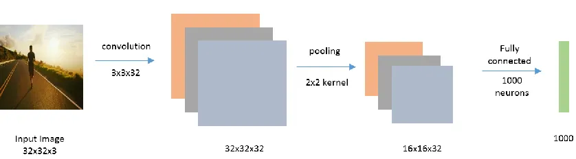
1.3.1 Convolutional Neural Network:
Convolutional neural networks have become the defacto-standard for the tasks of image
classification, segmentation and detection. Typically they comprise of the following layers:
Convolution layer
Pooling layer
Activation layer
Fully connected layer
A convolution layer consists of multiple filters which slide across the input image and
produce a linear response from filter weights applied to the input pixels. Each filter learns a
different set of representations of the original image eg: color, shape and edge information.
A pooling layer aggregates the information across a specified window in an image. The
two popular pooling approaches used are max pooling and average pooling. Max pooling
12
outputs the average intensity of the pixels. Performing pooling reduces the spatial dimensions
of the input.
An activation layer introduces non-linearity in the network. It helps to learn complex
representations that exist between input image and desired target in the network.
A fully connected layer is used as a final layer in most of the classification problems.
It is generally used to transform a high dimensional representation into an n-dimensional
representation by connecting all the pixels in the input layer to each neuron in the output layer.
During training, the filters of the convolutional layers and weights of fully connected
layers are learned by optimizing the cross entropy loss between predicted and groundtruth
labels of samples in classification problems. An example of a typical CNN is shown in Figure
[image:13.612.90.509.370.486.2]1.
Figure 1 An example Convolutional Neural Network.
1.3.2 Recurrent Neural Networks
Recurrent Neural Networks (RNN) have achieved significant success in time-series
problems and machine translation. A basic RNN unit consists of a hidden state and an input
which together predict the next state of a sequence. Some of the most popular variants of RNNs
are Gated Recurrent Units (GRU) and Long Short Term Memory (LSTM) units. LSTMs are
often the preferred choice for long sequences as they tend to remember long term dependencies
13
Figure 2 Basic LSTM cell [42].
where ct denotes the memory unit, ht denotes the hidden state, ft denotes the forget gate, it
denotes input gate and ot denotes the output gate.
The above gates followed by sigmoid and tanh activation units regulate the amount of
information that needs to be passed to the consecutive time steps in the network. More
commonly, LSTM networks are used in machine translation, which are otherwise known as
sequence-sequnce models.
𝑖𝑡 = 𝜎(𝑊𝑥𝑖𝑥𝑡+ 𝑊ℎ𝑖ℎ𝑡−1) (1)
𝑜𝑡 = 𝜎(𝑊𝑥𝑜𝑥𝑡+ 𝑊ℎ𝑜ℎ𝑡−1)
𝑓𝑡= 𝜎(𝑊𝑥𝑓𝑥𝑡+ 𝑊ℎ𝑓ℎ𝑡−1)
𝑔𝑡 = ∅(𝑊𝑥𝑐𝑥𝑡+ 𝑊ℎ𝑓ℎ𝑡−1)
𝑐𝑡 = 𝑓𝑡𝑐𝑡−1 + 𝑖𝑡𝑔𝑡
ℎ𝑡 = 𝑜𝑡∅(𝑐𝑡)
where it, ot, ft and gt are the input gate, output gate, forget gate and input node
14
the cell. The hidden state ht is passed to future timesteps in the network which contains the
[image:15.612.99.556.140.362.2]aggregate information of the previous timesteps.
Figure 3 Long Short Term Memory network with encoder and decoder chains [6].
Figure 3 shows an example of an encoder-decoder network with LSTM units. The
encoder and decoder may or may not share the same LSTM units. The encoder encodes the
input sequence “How are you”, one word at a time using a word embedding. The final state of
the encoder is the last hidden timestep of the input sequence. The encoder’s final time step is
passed along with a start token as input to the first timestep of the decoder. The decoder is
unrolled for variable timesteps and outputs a decoded sentence followed by an end token. This
15
Chapter 2
Related Work
2.1 Cross Modal Applications
Image captioning was one of the earliest works that demonstrated outstanding
capabilities of neural networks to generalize well on learning patterns in both vision and
language modalities. Neural networks trained with back propogation tend to learn patterns in
the image and correlate the relationships between objects in the image and individual words in
the sentence. The branch of study that deals with similarities between different entities is called
Metric Learning. The task of cross-modal retrieval involves learning similar representations
between two modalities. For example, given the two modalities of image and text, one can
extract meaningful content from a database given a query of either modality. Images have
diverse content and a sentence describing the image should capture not only the objects present
in the image but also the relationship between them. Often images can be described in many
ways and capturing the right context in the sentence is challenging. For example, “a man is
running” and “a man is not running” have most of words same but the word “not” changes the
entire meaning of the description. CNNs have become the defacto standard in representing
images and recurrent neural networks have been adept at capturing the syntactic and semantic
representations of the sentence. In this thesis, neural networks with latest CNN and RNN
architectures and current metric learning approaches are explored in cross-modal settings to
16
2.2 Current Metric Learning Approaches
Metric learning models involving images and text include:
Extracting features from images and text using CNNs and language models (Bag of
Words, LSTMs, skipgram)
Generate embeddings from these features using fully connected layers.
Form positive and negative pairing of data and use different loss functions for
convergence.
Some of the commonly used loss functions are:
1) Contrastive Loss
In contrastive learning, positive and negative pairs of the data are formed by the
distance between the image and caption encoding. Contrastive loss strives to have negative
pairs be at least a margin distance away from positive pairs. The loss function is as follows:
𝐿𝑐 = 2𝑁1 ∑((𝑦)𝑑2+ (1 − 𝑦) max(𝑚𝑎𝑟𝑔𝑖𝑛 − 𝑑, 0)2) (2)
where d is the distance between the vectors in a pair. The first term minimizes the distance between positive pairs, while the second term penalizes negative samples whose distance is
closer than a margin. The distance can be Euclidean, cosine, or other appropriate metric.
2) Triplet Loss
Triplets are formed by selecting an anchor sample and generating positive and negative
examples with respect to the anchor sample. The distance between the positive sample and the
anchor is minimized whereas the distance between the anchor and negative sample is
17 𝐿𝑐 = 1
2𝑁∑ max (0, |𝑓𝑎𝑖− 𝑓𝑝𝑖|
2
− |𝑓𝑎𝑖− 𝑓 𝑛𝑖|
2
+ 𝑚𝑎𝑟𝑔𝑖𝑛)
𝑁
𝑖=0
(3)
where fai is the feature embedding of the anchor, fpi is the feature embedding of positive sample
and fniis the feature embedding of negative sample. The triplet learning process is shown in
the Figure 4.
Figure 4 Optimizing latent space through triplet loss [12].
3) Lifted Structured Loss
Lifted structure loss extends the concept of triplet loss by considering multiple negative
samples for each positive sample. It ensures the distance between the positive and anchor
sample is less than distance between anchor and all other negative samples in the batch. The
lifted loss is defined as follows
𝐿𝑐 = 2|𝑃|1 ∑(𝑖,𝑗)∈Pmax (0, 𝐽i,j) (4)
where
18
where N denotes the set of negative samples and P denotes the set of positive samples.
Each sample is compared against a positive sample and all other negative samples in the batch
thereby forming tighter boundaries between samples during training.
Many approaches either use the above losses or the extensions of these to optimize the
distance between embeddings of different modalities. Most of the metric learning approaches
use labels as anchors to form positive and negative pairing. Two pictures of dogs are treated
as similar examples irrespective of their color, orientation and background, whereas a picture
of dog and cat are treated as negative pair.
On the contrary, in cross modal setting, there might not be labelled data with exclusive
categories for each image and captions. More naturally occurring images and text contain
multiple objects and various kind of actions describing their context. This poses a harder
challenge to distinguish samples of any specific category. The general consensus is that the
captions that were used to describe the image are treated as positive pairs and the rest of the
captions in a dataset are treated as negative pairs. This assumption makes the general metric
learning loss functions applicable to the problem of cross-modal retrieval.
2.3 Related Work
Koch et al. [17] introduced siamese networks to learn similarities between characters using contrastive loss and achieved superior performance on one-shot image recognition tasks.
Jiquan et al. [1] demonstrated that better features can be learned if multiple modalities are present during training. They also demonstrate a method to learn shared representations of
zero-19
shot recognition tasks. Schroff et al. [12] proposed triplet loss to enhance similatity learning by considering triplets of data and showed improved performance on face recognition. Hoffer
et al. [18] used triplet loss on metric learning problems and compared its performance to siamese networks which used contrastive loss. Song et al. [15] proposed lifted structured loss which essentially takes advantage of all the samples in the batch. For each positive sample, it
pushes all the negative samples away by a margin in a batch. This showed improved retrieval
performance on standard benchmark datasets. Euclidean distance is used as standard distance
metric in their experiments.
One of the most important aspect in similarity learning is the distribution of samples in
a batch and the strategy of forming positive and negative pairs within a batch. Not all the
negative samples are equally negative. During training, optimizing Euclidean loss of positive
and negative samples with respect to an anchor sample in a batch results in the formation of
discrete clusters in the high dimensional space. Negative samples can be classified into three
categories as follows
Hard negatives
Semi-hard negatives
20
Figure 5 Distrubution of negative samples [20].
Figure 5 shows the distrinution of negative samples with respect to an anchor sample.
Hard negative samples are closer to positive samples, semi-hard negatives lie within margin
distance from the positive samples and easy negatives already are far away from the anchor
sample under consideration. Hard negative mining is a strategy that mines the hardest negatives
for a given sample in a batch. Although hard negatives produce a high loss value, they also
produce high gradients which might lead to bad convergence of the model.
Exploiting the success of generative adversarial networks [16], Duan et al. [19] proposed to use a generator that exploits all easy negative samples and transforms them into
hard negative samples. A generator is trained adversarially to generate features which are
similar to features from hard negative samples thereby enhancing the training. A combination
21
discriminative features from the network and improved retrieval results compared to standard
metric loss functions. Figure 6 shows their model where the generator is a three layered fully
connected network which generates synthetic negative samples.
Figure 6 Deep Adversarial Metric Learning[19].
Schroff et al. [12] proposed to use semi-hard negative mining which samples only semi-hard negatives for each sample. They found loss to be decaying smoothly compared to
random negative sampling. Chao et al. [21] proposed a margin based loss and also proposed distance weighted sampling which selects negative samples based on their distances. They
show that learning the margin parameter removes the inherent bias that restricts all negative
samples to be pushed apart by a constant margin value.
2.4. Image-Text models
The main difference between metric learning and multi-modal learning is the encoding
22
can be expressed in the form of Euclidean distance between vector representations of these
images. This vectorization of images is generally a vector representation from a fully
connected layer of a CNN. The effectiveness of the CNN also plays an important factor in
learning discriminative features among images. In the context of multi-modal learning which
involves images and captions, separate encoders for each modality are required due to
difference in the structures. Images are encoded by CNN (image2vec) and a caption is passed
through an RNN (sent2vec). Aviv et al. [22] used two way neural networks to optimize Euclidean loss between images and text in a common embedding space. Vendrov et al. [23] proposed to use order-violation penalty to enforce constraint on the order in which the
embeddings are learned. In particular, they only use absolute value of image and text
embeddings and use margin-based loss to optimize the model.
Faghri et al. [23] proved hard negative mining can be useful and they showed significant improvements on cross modal retrieval problems. This is counterintuitive to metric
learning problems where hard negative mining hurts performance by ignoring semi-hard and
easy negative samples. Wehrmann et al. [25] proposed to use convolutional text encoders and perform convolutions over characters as opposed to words. They use an embedding matrix for
characters and show significant reduction in number of paramters of the model.
You et al. [26] propose to use local context along with global loss to train the image embeddings. Their method represents each word in a caption by learning a word embedding
matrix and perform series of 1-d convolutions over the individual words to get a final encoding
23
Figure 7 Convolutional Semantic Model [26].
Figure 7 shows their model which enforces a local loss between the intermediate
convolutional layers of images and text. The margin based ranking loss is used for aligning
both the local and global context.
Images consist of diverse content which can include objects as well as actions and
attributes describing them. Most of the commonly occurring datasets like MSCOCO [7] and
FLICKR 30K [27] contain only objects in the image and captions associated with them.
Objects alone do not convey the semantic meaning of the image. Extending this idea, Yan et al. [28] built a vocabulary consisting of image categories, attributes and actions using the captions corresponding to each image. A caption describing the image contains more semantic
information. Using the example “Two men are fighting on the road”, semantic entities include
“Two”, “men” , “fighting” and “road”. Nouns, adjectives and cardinal numbers are extracted
from each caption and frequently occurring words are treated as discrete classes. Using these
24
Figure 8 Image Sentence Matching using Multi-label CNN [28].
Figure 8 outlines their model where regions of an input image are passed to a
multi-label CNN. The class probabilities of the multi-multi-label CNN represent the distribution of
semantic concepts in the image. A gated fusion unit is used which takes the semantic concepts
and global features extracted by Resnet-152 [9] and outputs a fused vector representation
which effectively weighs the importance of global and local features. The architecture of the
gated fusion unit is similar to an LSTM cell where the sigmoid activation is applied to the
linear combination of inputs which regulates the amount of information passed from input
stage to the output stage. A Gated Recurrent Unit (GRU) is used as a sentence encoder where
consecutive words in a caption are passed at each timestep of the network. A sentence generator
is also used as supervision which ensures that the image can also generate the relevant caption.
The sentence generation and the margin based ranking loss can effectively guide the image to
better represent the content in the sentence during training. During inference, they extract ‘r’
regions from each test image and pass each region to a multi-label CNN The value of ‘r’ was
set to 50. Output class probabilities vectors are obtained for all the regions and they are
max-pooled. This results in a single vector which has the information of individual classes. The
gated fusion unit combines the aggregate class probabilities vector which has the local context
25
final image embedding for the test image. This mechanism of learning semantic concepts and
then matching it with the sentence embedding significantly improved the performance of
retrieval.
Martin et al. [38] proposed to use selective pooling of the convolutional feature maps in the setting of a two branch network to enhance cross modal retrieval. Figure 9 shows their
model where the selective pooling is applied at the pool block before the affine normalization
of the image embedding.
Figure 9 Selective pooling of convolutional feature maps for image-sentence matching [38].
Selective spatial pooling is given by (6):
ℎ[𝑘] = max 𝐺(: , ∶, 𝑘) + min 𝐺(: , ∶, 𝑘) , 𝑘 = 1 𝑡𝑜 𝐷′ (6)
where G is a convolutional feature map of size width x height x 𝐷′. 𝐷′ represents the number of feature maps of last layer of Resnet-152 [9]. The selective spatial pooling can be
considered as an aggregation of max pooling and min pooling. A simple recurrent unit (SRU)
26
parameters of Resnet-152 [9], SRU and the embedding layers are learned by optimizing the
margin based ranking loss between image and caption pairs.
Sah et al. [43] proposed a Common Vector Space (CVS) which brings similar concepts from different modalities closer in this space. They used different variants of metric learning
loss functions [12, 15, 17] during training to achieve a common latent representation between
images and text. One of the key difference between other methods is the way they infer the
embeddings from CVS. During inference, they use the embeddings from either modality to
27
Chapter 3
Methodology
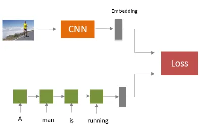
3.1 Baseline Model
[image:28.612.119.514.204.472.2]
Figure 10 Baseline Model.
In order to establish a CVS between images and text, we need encoders which extract
semantic information from individual modalities.Figure 10 shows the baseline architecture
which is used for cross modal retrieval in this research. An input image is passed through a
deep convolutional network [8, 9, 10] which extracts global features. These features are passed
through a fully connected layer whose output is the vector representation of the image in the
common embedding space. The sentence is encoded via GRU or LSTM and then passed into
28
embeddings which ensures similar concepts come closer and dissimilar concepts are pushed
far apart by at least margin in the common embedding space.
Margin based Ranking Loss
Face recognition has seen significant progress in recent years and most of it can be
attributed to metric learning loss functions that enhance the learning of the model. Several
novel loss functions have been proposed [15, 17, 18, 19, 21], which exploit the batch to form
exhaustive positive and negative pairs. Given a batch of samples, each sample is compared
against all other samples in the batch. The number of triplets that can be formed in a batch is
of the order O(n3). The number of contrastive pairs that can be formed in a batch is of the order
O(n2). Optimizing over all these combinations is computationally infeasible and pose heavy
memory constraints on fitting large models on standard GPUs. Sampling strategies such as
hard and semi-hard negative mining have thus been proposed to mitigate this issue. Equation
(7) shows an extension of triplet and lifted structured loss for cross modal tasks.
Lsim = ∑ ∑ max(0, 𝛼 − 𝑆(𝑖, 𝑐) + 𝑆(𝑖, 𝑐𝑚 𝑘 𝑘))+ ∑ ∑ max(0, 𝛼 − 𝑆(𝑐, 𝑖) + 𝑆(𝑐, 𝑖𝑘 𝑚 𝑘)) (7)
where is the margin of separation of positive and negative pairs, c denotes a caption and i denotes an image. In (7), ‘m’ denotes the total number of images and ‘k’ denotes the total number of sentences in a batch. The first term in the equation is associated with caption
retrieval where a single image is compared against all the ‘k’ captions in the batch. The second term in the equation is associated with image retrieval where each caption in the batch is
29
similarity between a caption and an image and S(i, c) computes the similarity between an image and caption. This similarity can be a cosine similarity as shown in (8) or we can use the order
violation penalty proposed in [23]. The order violation penalty enforces hierarchy of captions
over image given by (9). It is always computed with the caption embedding being the anchor.
The baseline model is a simplified model with all the necessary image and text pipelines.
𝑆(𝑖, 𝑐)𝑐𝑜𝑠𝑖𝑛𝑒 = 𝑖. 𝑐𝑇 (8)
𝑆(𝑖, 𝑐)𝑜𝑟𝑑𝑒𝑟 = 𝑚𝑎𝑥(0, |𝑐| − |𝑖|)2 (9)
where i, c denote the image and caption embeddings and |i| denotes the absolute value of the image embedding.
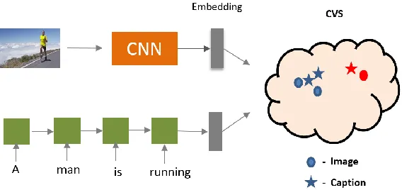
[image:30.612.157.441.485.619.2]3.2 Show, Translate and Tell (STT)
30
Figure 11 shows the CVS of images and text embeddings. CNNs and RNNs act as
encoders for images and text. Images and captions which are semantically similar are mapped
closer in this CVS. For example, in Figure 11, the image of a man running is eqiuvalently
described by the sentence “A man is running”. They are treated as positive pairs marked by
the blue circle and star in the Figure 11. The margin based ranking loss in (7) brings these
positive pairs closer and maps all the other negative pairs denoted by red circle and red star far
apart by atleast margin.
Figure 12 Show, Translate and Tell.
The baseline model constructs a CVS where the relationships between images and text
are expressed in terms of the similarity score between their respective embeddings. CVS is a
continuous space- without training, data points corresponding to images and text from the
original dataset would be mapped arbitrarily. Training CVS forms dense clusters of matching
images and captions. In order to explore the information contained in these CVS data points,
we need to decode them into meaningful representations. Modality specific decoders can
generate either images or captions. One of the early approaches related to this idea was
31
training. They use a pre-trained image generator [44] as decoder which accepts a 4096
dimensional vector as input to generate images. This limits the interpretability of CVS in that
the underlying distribution of CVS might be different from the input distribution that is
expected by the image generator. More often, the generated images experienced the
phenomenon of mode collapse. Inspired by [43] and image captioning models [29, 30, 31,
32], we propose Show, Translate and Tell (STT) which represents images and text in the CVS
and also decodes the embeddings into captions by using an RNN. Figure 12 shows the
schematic of the proposed model. STT offers a simple way to infer the embeddings in CVS by
using an RNN as a decoder which is trained along with the image and text encoders. This
ensures that decoder is aware of the distribution of the CVS embeddings. Since the output of
the decoder was intended to be paraphrase captions, RNN was the preferred choice to generate
these sentences.
During training, a single sample constitutes an image and two captions (caption A and
caption B) as shown in the Figure 12. The captions describe the contents of an image. Features
are extracted from image and caption ‘A’ using deep convolutional and recurrent networks.
These features are projected into a CVS which aligns similar images and captions.
Caption ‘B’ which is always semantically similar to caption ‘A’ is used to enhance the
overall quality of the model. The left side of the model in Figure 12 comprises of encoder
models which encode a modality into its corresponding representation. The right side of the
model is a recurrent neural network which acts as a decoder for both the image and caption A.
32
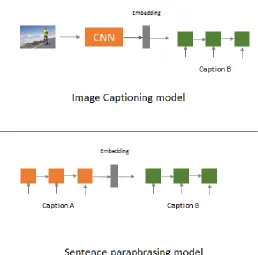
Figure 13 Image Captioner and Sentence Paraphraser.
Image sentence matching is closely related to sentence paraphrasing and image
captioning. In image captioning models, an input image is projected into its feature space and
passed to an RNN. During training, the RNN tries to correlate words in the sentence with the
objects and actions in the image. A vocabulary of words is built using the most frequently
occurring words in the captions. Each word in the vocabulary is encoded into a vector
representation by a randomly initialized word embedding matrix. The word embedding matrix
acts as a look-up table for the words in the caption. During training, the embedding matrix is
also learned along with the weights of RNN and CNN. This ensures the word embedding
matrix accurately learns the relationships between words and the underlying context within a
33
During training, the grountruth words are passed as input at current timestep instead of
the word predicted by previous timestep. Cross-entropy loss between the predicted words from
each timestep of RNN and the groundtruth sentence is used to optimize the parameters of the
model. During testing, an image is passed through the network along with a start token for
decoding the words in the sentence. Equation (10) denotes the loss that is used to train an image
captioner.
LIC= − ∑𝑁𝑡=1log 𝑃(𝑆𝑡|𝐼; 𝜃) (10)
where P(St) is the probability of observing the correct word St at time t, denotes the
paramters of the model and I denotes the image features.
Sentence paraphrasing models transforms a caption ‘A’ into caption ‘B’ which is
semantically similar to caption ‘A’. The words in the caption are encoded into vector
representations by the embedding matrix. Sentence paraphrasing models are modeled in
encoder-decoder framework where both encoder and decoder use recurrent neural networks.
During testing, the input to the model is the encoded sentence representation by the encoder
along with the start token. Equation (11) denotes the cross entropy loss used to train the
sentence paraphraser.
Lpara = − ∑𝑁𝑡=1log 𝑃(𝑆𝑡|𝐸; 𝜃) (11)
where Pt(St) is the probability of observing the correct word St at time t, E denotes the
encoder representation of the sentence and 𝜃 denotes the paramters of the model.
The sentence paraphrasing model ensures the two sentences are closer in the embedding space.
34
into a similar representation. Combining the benefits of the image captioning model and
sentence paraphrasing model, Figure 12 is a unified model which can perform three different
tasks namely image-caption retrieval, image captioning and sentence paraphrasing.
Equation (12) shows the loss for the unified model.
𝐿 = 𝜆1𝐿𝐼𝐶+ 𝜆2𝐿𝑝𝑎𝑟𝑎+ 𝜆3𝐿𝑠𝑖𝑚 (12)
where LIC, Lpara and Lsim correspond to the image captioning, sentence paraphrasing
and similarity loss respectively. 𝜆1, 𝜆2 and 𝜆3are the weights for each of the components of
35
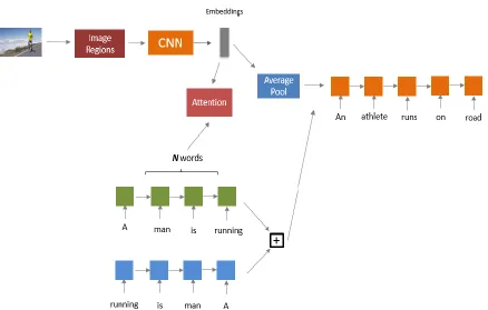
3.3 STT with Attention
Figure 14 Show, Translate and Tell model with Attention.
Figure 14 describes the Show, Translate and Tell model with attention. The input
image is passed through an object detector which outputs region proposals with objectness
score in the image. The object detector used in this process is Faster R-CNN [36] which is a
two-stage object detection network. In the first stage, it outputs region proposals with amount
of objectness in each of them. These proposals are later refined in the second stage and
bounding box regressor head localizes the objects in the image. The number of proposals after
the first stage is 300. We consider a subset of ‘M’ of these proposals based on their objectness
score and extract the portions in the original image. These extracted proposals are passed
36
our experiments, we set the value of ‘M’ to be 36. For more local information and semantic
understanding of the contents in the image, we follow [37] to introduce attention between the
region proposals in the image and individual words in the sentence. The similarity matrix
introduced by [37] calculates the similarity between regions in the image and words in the
sentence and is given by
𝑠𝑖𝑗 = 𝑣𝑖
𝑇𝑒 𝑗
||𝑣𝑖|| ||𝑒𝑗|| (13)
where sij is the similarity between ith region (vi) and jthword (ej). Based on the above
similarity matrix, an attended sentence vector is calculated as
ai𝑡 = ∑ 𝛼𝑖𝑗𝑒𝑗
𝑛
𝑗=0 (14)
where
𝛼
𝑖𝑗=
exp (𝜆1𝑠𝑖𝑗)∑𝑛𝑗=1exp (𝜆1𝑠𝑖𝑗)
(15)
𝛼
𝑖𝑗 is the attention weights which calculates the importance of each word in thesentence with respect to ith region. The similarity between an image and text is then defined as
a mean of similarity between image regions and attended sentence vectors. Equation 16 shows
the aggregate similarity score between an image and a text.
𝑆(𝐼, 𝑇) = ∑ 𝑅(𝑣𝑖,𝑎𝑖
𝑡) 𝑘
𝑖=1
37
where R(vi, ait ) is the similarity of ith image region and attended sentence vector
given by
𝑅(𝑣𝑖, 𝑎𝑖𝑡) = 𝑣𝑖𝑇𝑎𝑖𝑇
|𝑣𝑖| |𝑎𝑖𝑡| (17)
This way of calculating similarity between regions in the image and words can be
directly plugged into (7) where the similarity of the negative pairs is reduced thereby bringing
the positive samples closer in the common embedding space. One difference between this
attention model and STT is that a single image is represented by multiple region embeddings
rather than a single feature vector. We add an average pooling layer which aggregates these
multiple region embeddings into a single representation which can be used as an input to the
decoder. The joint training of the decoder and individual image and text encoders along with
the attention model helps in aligning the image regions with the individual words and also in
38
Chapter 4
Implementation and Results
4.1 Datasets
Some of the popular cross modal datasets which include images and captions associated
with them include
MSR-VTT [33]
Caltech-UCSD Birds 200 [4]
Flowers 102 dataset [3]
MSCOCO [7]
FLICKR 30K [27]
MSR-VTT [33] is a large scale video to text dataset which bridges video and language.
It has comprehensive categories and diverse video content which can be used for video
retrieval, event detection tasks.
Caltech-UCSD Birds 200 [4] is a medium scale dataset consisting of 200 categories of
birds along with attributes for each image. Each image is also annotated with 10 captions which
describe the content in the image.
Flowers 102 [3] dataset is a dataset by University of Oxford which consists of 102
different categories of flowers with 10 captions associated with each image.
MSCOCO [7] dataset is a large-scale dataset comprised of common objects that are
found in nature. It is widely used for multi-label classification, object detection, semantic
39
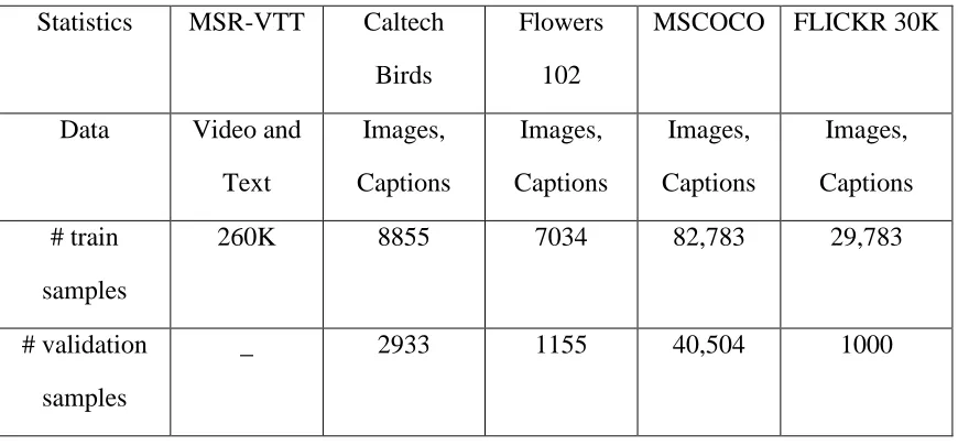
Table 1 Summary of cross-modal datasets.
This work focuses on bridging natural image content and corresponding descriptions.
Caltech-UCSD Birds dataset [4] and Flowers 102 dataset [3] are very specific to birds and
flowers and the diversity of the dataset in terms of datasets and semantic content is limited.
These datasets are more oriented towards zero shot image retrieval and classification.
MSR-VTT [33] is more suitable for temporal video analysis, video segmentation and captioning. In
this work, MSCOCO [7] and FLICKR 30K [27] datasets are explored which contain real-world
images with short descriptions associated with them.
4.2 Training Details
Each image is passed through a Resnet-152 CNN [9] and features are extracted from
the global average pooling layer. For the embedding network, we use a single fully connected
layer. Training is performed in multiple stages. In the first stage, we pre-compute the features
from Resnet-152 [9] and train the image embedding and sentence encoder from scratch for 15
epochs with a learning rate of 0.0002 and lower the learning rate to 0.00002 for the next 15 Statistics MSR-VTT Caltech
Birds
Flowers
102
MSCOCO FLICKR 30K
Data Video and
Text Images, Captions Images, Captions Images, Captions Images, Captions # train samples
260K 8855 7034 82,783 29,783
# validation
samples
40
epochs. We use Adam optimizer for optimizing the parameters of the model. Once we have
the model trained with the precomputed features, we finetune the Resnet-152 CNN along with
embedding layers and sentence encoder with a learning rate 0.00002 for another 15 epochs.
We found the model to be highly sensitive to the learning rate and higher learning rates often
led to model getting stuck at local minimum. We use Tensorflow deep learning framework for
all our experiments.
For the sentence representation, we use a 1-layer GRU network. The hidden dimension
of the GRU was set to 1024. We experimented by stacking more layers, but there was no
significant improvement by introducing more parameters. This complemented with our usage
of only one fully connected layer for generating embeddings. The vocabulary of words was
built by counting the frequency of all the words in the captions present in the dataset. A word
is considered to exist in vocabulary if the frequency of its occurrence is greater than three. The
size of the vocabulary is 26,375 words. The word embedding dimension was set to 300.
For the margin based ranking loss, we set the margin to 0.05 and we use order violation
penalty [23] for computing the similarity metric. The batch size is set to 128, so the number of
contrastive examples for each matching pair would be 127. We employ hard negative mining
where we only consider the hardest negative distance instead of aggregating all the negative
distances. We noticed a significant performance improvement in retrieval with hard negative
mining strategy.
41
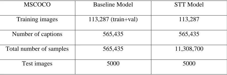
Table 2 MSCOCO statistics.
MSCOCO Baseline Model STT Model
Training images 113,287 (train+val) 113,287
Number of captions 565,435 565,435
Total number of samples 565,435 11,308,700
Test images 5000 5000
For the baseline model, a sample constitutes an image and caption. Since each image
is associated with a set of five captions, the training set of images constitute 565,435 samples
in total. For the STT model, a sample constitutes an image and two similar captions. Since we
have five captions associated with each image, there can be 20 different combinations. Hence,
the total number of samples for the STT model would be 11,308,700.
[image:42.612.92.522.112.255.2]Table 3 shows the statistics for FLICKR 30K dataset that we used in our experiments.
Table 3 FLICKR 30K statistics.
FLICKR 30K Baseline Model STT Model
Training images 29,783 29,783
Number of captions 148,915 148,915
Total number of samples 148,915 2,978,300
Test images 1000 1000
For the baseline model, a sample constitutes an image and caption. Since each image
is associated with a set of five captions, the training set of images constitute 148,915 samples
42
have five captions associated with each image, there can be 20 different combinations. Hence,
the total number of samples for the STT model would be 2,978,300.
4.3 Evaluation Metrics
The following evaluation metrics are used as a standard to compare the performance of
cross-modal retrieval.
4.3.1 Recall@K
Recall@K computes the recall at different values of K. It is a metric which computes if the rank of retrieved sentence is within the top K ranks. All the test set images and their associated captions are passed through the model and their embeddings are extracted. Each
image embedding in the test set is compared with all other caption embeddings and similarity
metric is computed. The similarity is sorted in descending order and appropriately all other
captions are ranked. If the rank of the groundtruth sentence is within the top K ranks, the caption is counted as a positive retrieval. Typical values of K are 1, 5 and 10. The overall recall score is the percentage of samples within the top K ranks.
For the image retrieval, we rank all images in the test set with every caption. The images
are sorted in descending order with respect to the similarity with respect to query caption and
ranked. If the rank of the groundtruth image is within the top K ranks, the image is counted as a positive retrieval.
4.3.2 Median rank
After computing the ranks for each samples, the median of these ranks is computed.
Ideally the median value should be 1 which implies all the samples should be correctly
43
4.3.3 Mean rank
Mean rank is the mean of the ranks of all samples in the test set. The mean rank should
also be equal to 1 in the perfect scenario where all the samples are correctly retrieved.
4.4 Baseline Results
4.4.1 MSCOCO
Table 4 Results of MSCOCO sentence retrieval using baseline model.
Table 5 Results of Image retrieval on MSCOCO test set using baseline model.
Variant Model Emb dim R@1 R@5 R@10 Med R Mean R
Baseline 1 FC 1024 41.4 75.1 85.9 2 12.2
Baseline 1 FC 2048 42.5 76 86.5 2 11.6
Tables 4 and 5 show the results of sentence retrieval and image retrieval on MSCOCO
dataset using the baseline model. The model configuration indicated in the tables is ‘1 FC’
which indicates that the image and text branches consist of one fully connected layer each.
The column ‘Emb dim’ indicates the size of the image and text embeddings. The network
architecture comprises of a Resnet-152 layer CNN for encoding images and GRU recurrent Variant Model Emb dim R@1 R@5 R@10 Med R Mean R
Baseline 1 FC 1024 55.5 85.2 92.3 1 4.6
44
network for encoding captions. From Table 4 and Table 5, we can conclude that increasing the
embedding dimension does not significantly affect the retrieval performance. There is a slight
improvement in other metrics.
The recall scores increase as we increase the values of K. This implies that there are significant number of retrievals within the top 10 ranks. The recall values of sentence retrieval
are comparatively higher than image retrieval due to the fact that each image is associated with
five different captions. A sentence retrieval is considered a positive retrieval if the retrieved
sentence belongs to any of the five associated captions for the image. In the image retrieval
case, each caption is associated with only one image which makes the problem more
challenging. This is evident from the R@1 scores of sentence and image retrieval which are
55.5 and 41.4 respectively.
4.4.2 FLICKR 30K
Table 6 Results of Sentence Retrieval using Baseline model on FLICKR 30K dataset.
Variant Model Emb dim R@1 R@5 R@10 Med R Mean R
Baseline 1 FC 1024 40.2 67.1 79.4 2 15.442
Baseline 1 FC 2048 38.4 67.4 77.5 2 13.4
Table 6 shows the results of sentence retrieval using baseline model on FLICKR 30K
dataset. The recall scores are comparatively lower than that of MSCOCO due to fewer samples
in the dataset. The model quickly overfits the training data hurting the performance on the test
set. We tackle overfitting by monitoring the model’s performance on validation data and
45
Table 7 Results of Image Retrieval using Baseline model on FLICKR 30K dataset.
Variant Model Emb dim R@1 R@5 R@10 Med R Mean R
Baseline 1 FC 1024 27.42 55.58 67.9 4 28.98
Baseline 1 FC 2048 27.1 55.9 68.2 4 24.5
Table 7 shows the results of image retrieval using Baseline model on FLICKR 30K
dataset. The recall scores are considerably lower compared to MSCOCO due to less number
of samples. From Tables 6 and 7, it is clear that increasing the size of embedding does not help
the performance of the retrieval model.
4.5 Results of STT Model
4.5.1 MSCOCO
Table 8 STT results on MSCOCO for Sentence Retrieval.
Variant Model Emb dim R@1 R@5 R@10 Med R Mean R
STT 1 FC 1024 54.7 83.6 92.1 1 4.5
STT 1 FC 2048 55.1 83.5 91.8 1 4.5
Table 8 shows the results of STT on MSCOCO for sentence retrieval. The model
configuration indicated in the tables is ‘1 FC’ which indicates that the image and text branches
consist of one fully connected layer each. The column ‘Emb dim’ indicates the size of the
image and text embeddings. The recall scores seem improve by 0.4% when the embedding
46
be that the model is overfitting the data since the new dataset for STT is 20 the original
image-caption pairs with many repetitive pairs as indicated in Table 3.
Table 9 STT results on MSCOCO for Image Retrieval.
Variant Model Emb dim R@1 R@5 R@10 Med R Mean R
STT 1 FC 1024 41 74.8 86 2 9
STT 1 FC 2048 41.3 75.2 86 2 9.3
Table 9 shows the results of STT on MSCOCO for image retrieval. The recall scores
do not seem to improve significantly with the increase in embedding dimension.
Image Captioning
The STT model is flexible and can perform diverse tasks. The top part of STT shown
in Figure 13 can effectively be used as an image captioner. The task of image-sentence
matching is performed by representing images and text close to each other in the common
embedding space. This high dimensional space is comprised of many naturally occurring
images and text that lie outside of the dataset. Our image captioner effectively generates
sentences which lie near the vicinity of the corresponding images. Table 10 shows the results
of image captioning on MSCOCO 1K test set.
Table 10 Image Captioning Results of STT model on MSCOCO 1k test set.
Variant Emb dim B@1 B@2 B@3 B@4 METEOR CIDEr
STT 1024 0.683 0.506 0.362 0.259 0.236 0.850
47
Table 10 indicates that the STT model is able to achieve good image captioning scores.
The effect of embedding dimension is clearly less significant in image captioning when
compared to cross modal retrieval.
Sentence Paraphrasing
The task of sentence paraphrasing model involves generating a paraphrase which is
semantically similar to the input sentence. This task is particularly challenging due to the fact
that a sentence can be described in many ways. The generated sentence should not only capture
the context of a sentence but it should also be syntactically different from the input sentence.
We evaluate our STT model on the task of sentence paraphrasing. Table 11 shows the result
[image:48.612.88.541.416.504.2]of sentence paraphrasing on MSCOCO 1K test set.
Table 11 Sentence paraphrasing results on MSCOCO 1K test set using STT model.
Variant Emb dim B@1 B@2 B@3 B@4 METEOR CIDEr
STT 1024 0.744 0.578 0.435 0.324 0.275 1.10
STT 2048 0.734 0.568 0.426 0.317 0.270 1.069
From Table 11, it is clear that the STT model can generalize well on sentence
paraphrasing tasks. It is able to obtain good scores which can be attributed to the fact that we
are jointly training the model on sentence paraphrases which contain more context. The
sentence decoder in STT model effectively makes sure the embeddings in the common vector
48
Visualizations
[image:49.612.101.307.170.316.2]1) Good examples
49
Figure 16 Sample STT output on MSCOCO.
Figures 15 and 16 show STT outputs on a sample images. From the figures, we can
observe that the top 3 retrieved sentences are a part of the groundtruth sentences for the image.
This indicates that the STT model was able to retrieve sentences very well. The image
captioning and sentence paraphrasing results also describe the image well.
2) Bad examples
50
Figure 17 shows an example where STT model failed to retrieve the right captions. The
retrieved captions describe content related to a group of animals and giraffes. This might be
due to the texture formed by the wooden spoons on the table as well as resulting color similar
to the color of giraffes. The captioning and paraphrasing show good results even though the
[image:51.612.93.529.222.389.2]retrieval failed.
Figure 18 Sample STT output on MSCOCO.
Figure 18 shows an example of ambiguous retrieval. Although the retrieved sentences
for the query image are semantically related to the image, they do not belong to the groundtruth
sentences which makes this a negative retrieval. The retrieved captions might be related to
another image with similar content. This example depicts that the cross-modal retrieval is very
challenging when there is high overlap of semantic content in the dataset.
[image:51.612.89.541.625.714.2]4.5.2 FLICKR 30K
Table 12 Sentence Retrieval results on FLICKR 30K dataset using STT model.
Variant Model Emb dim R@1 R@5 R@10 Med R Mean R
STT 1 FC 1024 38.9 66.9 78.4 3 13.3
51
Table 13 Results of Image Retrieval on FLICKR 30K dataset using STT model.
Variant Model Emb dim R@1 R@5 R@10 Med R Mean R
STT 1 FC 1024 27.2 55.4 68.4 4 27.6
STT 1 FC 2048 27.1 55.9 68.2 4 24.5
Table 12 and 13 show the results of sentence retrieval and image retrieval on FLICKR
30K using STT model. STT model’s performance is lower than the baseline model for retrieval
but still shows strong performance. STT results on FLICKR 30K [27] are consistent with
[image:52.612.88.550.368.456.2]MSCOCO [7].
Table 14 Results of Image Captioning on FLICKR 30K using STT model.
Variant Emb dim B@1 B@2 B@3 B@4 METEOR CIDEr
STT 1024 0.513 0.330 0.204 0.129 0.178 0.252
[image:52.612.87.547.514.603.2]STT 2048 0.508 0.323 0.198 0.124 0.167 0.216
Table 15 Results of Sentence Paraphrasing on FLICKR 30K using STT model.
Variant Emb dim B@1 B@2 B@3 B@4 METEOR CIDEr
STT 1024 0.569 0.394 0.262 0.176 0.217 0.398
STT 2048 0.548 0.364 0.233 0.151 0.189 0.292
Tables 14 and 15 show the results of image captioning and sentence paraphrasing on
FLICKR 30K [27] using STT model. As the embedding dimension is increased, the scores
52
Visualizations
1) Good examples
Figure 19 Sample STT output on FLICKR 30K.
Figure 19 shows an example of a good retrieval for a query image. The sentence ‘A man surfing in the ocean’ is repeated twice in the dataset and they belong to two different image samples. Captioning results describe the image in more detail although the syntax is
slightly affected. The paraphrasing also outputs good results and shows good diversity.
2) Bad examples
53
Figure 20 shows the results of a failed retrieval on FLICKR 30K [27] dataset. The
retrieved captions do not belong to set of groundtruth captions. However, the retrieved captions
describe the image accurately. This ambiguity can be attributed to the positive and negative
pairing in the dataset during training. Since there is a significant overlap between some samples
in the training data, the strict definition of each sample being a negative to all other samples in
the dataset results in such ambigious scenarios.
4.5.3 Cross Domain Evaluation of STT model
In order to explore the generalization performance of STT model on other datasets, we
perform cross-domain evaluation. We evaluate the STT model trained on MSCOCO [7], on
[image:54.612.95.519.379.469.2]FLICKR 30K [27] and vice-versa.
Table 16 Transfer learning results of STT model on Sentence Retrieval.
Variant Model Emb dim R@1 R@5 R@10
STT MSCOCO-FLICKR 30K 1024 32.9 57.4 67.4
STT FLICKR 30K-MSCOCO 1024 24.8 50.5 62.4
Table 17 Transfer learning results of STT model on Image Retrieval.
Variant Model Emb dim R@1 R@5 R@10
STT MSCOCO-FLICKR 30K 1024 21.1 43.5 55.4
STT FLICKR 30K-MSCOCO 1024 17 41.3 55.3
Tables 16 and 17 show transfer learning results of STT model on sentence and image retrieval.
The model configuration ‘MSCOCO-FLICKR 30K’ indicates that the model was trained on
MSCOCO [7] and evaluated on FLICKR 30K [27] dataset. The model ‘MSCOCO-FLICKR
54
MSCOCO [7] dataset. This can be due to the fact that the MSCOCO [7] dataset is a much
larger dataset as compared to FLICKR 30K [27] dataset. Since MSCOCO [7] and FLICKR
30K [27] have similar type of objects and content in the images, transfer learning is a good
mechanism to evaluate the overall performance of the model.
4.6 Results of STT Model with Attention
4.6.1 MSCOCO
Table 18 Results of Sentence Retrieval on MSCOCO dataset using STT with Attention.
Variant Emb dim R@1 R@5 R@10 Med R Mean R
[image:55.612.117.517.406.466.2]STT-ATT 1024 64.9 91 96.8 1 2.5
Table 19 Results of Image Retrieval on MSCOCO dataset using STT with Attention.
Variant Emb dim R@1 R@5 R@10 Med R Mean R
STT-ATT 1024 49.8 83 91.6 1 5.6
Tables 18 and 19 show the results of sentence and image retrieval on MSCOCO using
STT model with attention (indicated by STT-ATT in the tables). As observed by [37], the
retrieval scores show a significant improvement with attention. This concludes that
cross-modal retrieval is a challenging task which requires fine-grained matching between images and
captions.
Table 20 shows the results of image captioning on MSCOCO using STT model with
attention. The table clearly shows improvement in the captioning scores over the STT model.
55
have local information about the objects in the image. The improvement in B@1 score with
respect to STT model is 2.3%.
Table 20 Image captioning results on MSCOCO 1K test set using STT with attention.
Variant Emb dim B@1 B@2 B@3 B@4 METEOR CIDEr
STT-ATT 1024 0.706 0.530 0.385 0.279 0.246 0.908
[image:56.612.93.537.265.324.2]
Table 21 Sentence paraphrasing results on MSCOCO 1K test set using STT with Attention.
Variant Emb dim B@1 B@2 B@3 B@4 METEOR CIDEr
STT-ATT 1024 0.747 0.581 0.436 0.326 0.272 1.098
Table 21 shows the results of sentence paraphrasing on MSCOCO 1K test set using
STT model with attention. The results are also complementary to image captioning results and
show improvement over the STT.
Visualizations
[image:56.612.115.525.421.690.2]1) Good examples
56
Figure 22 Sample output of STT-ATT model on MSCOCO.
Figures 21 and 22 show good outputs of STT model with Attention on MSCOCO [7].
The retrieval results seem perfect and the outputs of captioning and paraphrasing captured
the semantic content in the image.
2) Bad examples
57
[image:58.612.125.524.77.259.2]
Figure 24 Sample STT-ATT output on MSCOCO.
Figures 23 and 24 show some failed retrievals of STT with Attention. In Figure 23, the
model retrieves captions related to train and station. The image embeddings might not have
been rich enough and the model confused the buildings with windows on a train. In Figure 24,
the model is confused with the number of women in the picture. Although the retrieved
captions reasonably describe the action of the woman, the groundtruth captions are different.
These kind of examples are particularly challenging due to the high overlap between content
in the data samples.
4.6.2 FLICKR 30K
Table 22 Results of Sentence Retrieval on FLICKR 30K dataset using STT with Attention.
Variant Emb dim R@1 R@5 R@10 Med R Mean R
[image:58.612.88.509.657.714.2]STT-ATT 1024 59.2 83.5 91 1 6.6
Table 23 Results of Image Retrieval on FLICKR 30K dataset using STT with Attention.
Variant Emb dim R@1 R@5 R@10 Med R Mean R
![Figure 2 Basic LSTM cell [42].](https://thumb-us.123doks.com/thumbv2/123dok_us/65811.6226/14.612.200.418.75.271/figure-basic-lstm-cell.webp)
![Figure 3 Long Short Term Memory network with encoder and decoder chains [6].](https://thumb-us.123doks.com/thumbv2/123dok_us/65811.6226/15.612.99.556.140.362/figure-long-short-memory-network-encoder-decoder-chains.webp)
![Figure 5 Distrubution of negative samples [20].](https://thumb-us.123doks.com/thumbv2/123dok_us/65811.6226/21.612.152.441.73.335/figure-distrubution-of-negative-samples.webp)