Intelligent Big Multimedia Databases pdf

(1)

(2)

(3)

b1816 MR SIA: FLY PAST b1816_FM

b1816_FM.indd vi

b1816_FM.indd vi 10/10/2014 1:12:39 PM10/10/2014 1:12:39 PM

(4)

(5)

Published by

:RUOG6FLHQWL¿F3XEOLVKLQJ&R3WH/WG 7RK7XFN/LQN6LQJDSRUH

86$RI¿FH:DUUHQ6WUHHW6XLWH+DFNHQVDFN1-8.RI¿FH6KHOWRQ6WUHHW&RYHQW*DUGHQ/RQGRQ:&++(

British Library Cataloguing-in-Publication Data

$FDWDORJXHUHFRUGIRUWKLVERRNLVDYDLODEOHIURPWKH%ULWLVK/LEUDU\

INTELLIGENT BIG MULTIMEDIA DATABASES &RS\ULJKWE\:RUOG6FLHQWL¿F3XEOLVKLQJ&R3WH/WG

$OOULJKWVUHVHUYHG7KLVERRNRUSDUWVWKHUHRIPD\QRWEHUHSURGXFHGLQDQ\IRUPRUE\DQ\PHDQV HOHFWURQLFRUPHFKDQLFDOLQFOXGLQJSKRWRFRS\LQJUHFRUGLQJRUDQ\LQIRUPDWLRQVWRUDJHDQGUHWULHYDO

system now known or to be invented, without written permission from the publisher.

)RUSKRWRFRS\LQJRIPDWHULDOLQWKLVYROXPHSOHDVHSD\DFRS\LQJIHHWKURXJKWKH&RS\ULJKW&OHDUDQFH &HQWHU,QF5RVHZRRG'ULYH'DQYHUV0$86$,QWKLVFDVHSHUPLVVLRQWRSKRWRFRS\ LVQRWUHTXLUHGIURPWKHSXEOLVKHU

,6%1

3ULQWHGLQ6LQJDSRUH

(6)

for Manuela

(7)

b1816_FM.indd vi

b1816_FM.indd vi 10/10/2014 1:12:39 PM10/10/2014 1:12:39 PM

(8)

Preface

Multimedia databases address a growing number of commercially impor-tant applications such as media on demand, surveillance systems and med-ical systems. The book will present essential and relevant techniques and algorithms for the development and implementation of large multimedia database systems.

The traditional relational database model is based on a relational alge-bra that is an offshoot of first-order logic and of the algealge-bra of sets. The simple relational model is not powerful enough to address multimedia data. Because of this, multimedia databases are categorized into many major ar-eas. Each of these areas are now so extensive that a major understanding of the mathematical core concepts requires the study of different fields such as information retrieval, digital image processing, fractals, machine learning, neuronal networks and high-dimensional indexing. This book unifies the essential concepts and recent algorithms into a single volume.

Overview of the book

The book is divided into ten chapters. We start with some examples and a description of multimedia databases. In addressing multimedia informa-tion, we are addressing digital data representations and how these data can be stored and manipulated. Multimedia data provide additional function-ality than would be available in traditional forms of data. It allows new data access methods such as query by images in which the most similar image to the presented image is determined.

In the third chapter, we address the basic transform functions that are required when addressing multimedia databases, such as Fourier and cosine transforms as well as the wavelet transform, which is the most popular.

(9)

April 7, 2015 16:32 ws-book9x6 9665-main page viii

viii Intelligent Big Multimedia Databases

Starting from continuous wavelet transforms, we investigate the discrete fast wavelet transform for images, which is the basis for many compres-sion algorithms. It is also related to the image pyramid, which will play an important role when addressing indexing techniques. We conclude the chapter with a description of the Karhunen-Lo`eve transform, which is the basis of principal component analysis (PCA) and the k-means algorithm.

The size of a multimedia object may be huge. For the eﬃcient storage and retrieval of large amounts of data, a clever method of encoding the information using fewer bits than the original representation is essential. This is the topic of the fourth chapter, which addresses compression algo-rithms. In addition to lossless compression, where no loss of information is present, lossy compression based on human perceptual features is essential for humans, and in this form of compression, we only represent the part of information that we experience.

Lossy compression is related to feature extraction, which will be de-scribed in the ﬁfth chapter. We introduce the basic image features and outgoing from the image pyramid, and for the scale space, we describe the scale-invariant feature transform (SIFT). Next, we turn to speech and explain the speech formant frequencies. A feature vector represents the extracted features that describe multimedia objects. We introduce the dis-tinction between the nearest neighbor similarity and the epsilon similarity for vectors in a database. When the features are represented by sequences of varying length, time wrapping is used to determine the similarity between them.

For the fast access of large data, divide and conquer methods are used, which are based on hierarchical structures, and this is discussed in the sixth chapter. For numbers, a tree can be used to prune branches in the process-ing queries. The access is fast: it is logarithmic in relation to the size of the database representing the numbers. Usually, the multimedia objects are described by vectors rather than by numbers. For low-dimensional vectors, metric index trees such as kd-trees and R-trees can be used. Alternatively, an index structure based on space-ﬁlling curves can be constructed.

The metric index trees operate eﬃciently when the number of dimen-sions is small. The growth of the number of dimendimen-sions has negative impli-cations for the performance of multidimensional index trees; these negative eﬀects are called the “curse of dimensionality.” The “curse of dimensional-ity”, which states that for an exact nearest neighbor, any algorithm for high dimensiondand nobjects must either use annd_{-dimension space or have}

(10)

Preface ix

indexing, the data points that may be lost at some distances are distorted. Approximate indexing seems to be, in some sense, free from the curse of dimensionality. We describe the popular locality-sensitive hashing (LSH) algorithm in the seventh chapter.

An alternative method, which is based on exact indexing, is the generic multimedia indexing (GEMINI) and is introduced in the eighth chapter. The idea is to determine a feature extraction function that maps the high-dimensional objects into a low-high-dimensional space. In this low-high-dimensional space, a so-called “quick-and-dirty” test can discard the non-qualifying ob-jects. Based on the ideas of the image pyramid and the scale space, this approach can be extended to the subspace tree. The search in such a struc-ture starts at the subspace with the lowest dimension. In this subspace, the set of all possible similar objects is determined. The algorithm can be easily parallelized for large data. Chunks divide the database; each chunk may be processed individually by ten to thousands of servers.

In the following chapter, we address information retrieval for text databases. Documents are represented as sparse vectors. In sparse vectors, most components are zero. To address this, alternative indexing techniques based on random projections are described.

The tenth chapter addresses an alternative approach in feature extrac-tion based on statistical supervised machine learning. Based on percep-trons, we introduce the back-propagation algorithm and the radial-basis function networks, where both may be constructed by the support-vector-learning algorithm. We conclude the book with a chapter about applica-tions in which we highlight some architecture issues and present multimedia database applications in medicine.

The book is written for general readers and information professionals as well as students and professors that are interested in the topics of large mul-timedia databases and want to acquire the required essential knowledge. In addition, readers interested in general pattern recognition engineering can proﬁt from the book. It is based on a lecture that was given for several years at the Universidade de Lisboa.

My research in recent years has beneﬁted from many discussions with ˆ

(11)

April 7, 2015 16:32 ws-book9x6 9665-main page x

x Intelligent Big Multimedia Databases

Finally, I would like to thank my sonAndr´e and my loving wifeManuela, without their encouragement the book would be never ﬁnished.

(12)

Introduction

Multimedia databases are employed in an increasing number of commer-cially important applications, such as media-on-demand, surveillance sys-tems and medical syssys-tems. Multimedia databases divide a subject into numerous major areas. Because each area is extensive, a major under-standing of the mathematical core concepts requires an investigation of the diﬀerent areas. In this book, we attempt to unify the essential concepts and recent algorithms.

1.1 Intelligent Multimedia Database

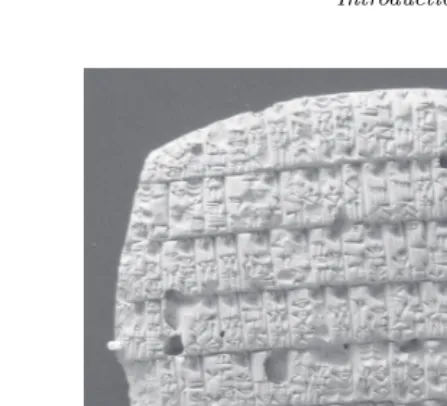
During prehistoric times and prior to the availability of written records, humans created images using cave paintings that were frequently located in areas of caves that were not easily accessible, as shown in Figure 1.1. These paintings were assumed to serve a religious or ceremonial purpose or to represent a method of communication with other members of the group [Curtis (2006); Dale (2006)]. As human societies emerged, the devel-opment of writing was primarily driven by administrative and accounting purposes. Approximately six thousand years ago, the complexity of trade and administration in Mesopotamia outgrew human memory. Writing be-came a necessity for recording transactions and administrative tasks [Wells (1922); Rudgley (2000)]. The earliest writing was based on pictograms; it was subsequently replaced by letters that represented linguistic utter-ances [Robinson (2000)]. Figure 1.2 displays a Sumerian clay tablet from 4200 years ago; it documents barley rations issued monthly to adults and children [Edzard (1997)]. Approximately 4000 years ago, the “Epic of Gil-gamesh”, which was one of the ﬁrst great works of literature, appeared. It is a Mesopotamian poem about the life of the king of Uruk [Sandars

(19)

April 7, 2015 16:32 ws-book9x6 9665-main page 2

2 Intelligent Big Multimedia Databases

Fig. 1.1 Reproduction of a prehistoric painting that represents a bison of the cave of Altamira near Santander in Spain.

(20)

[image:20.595.94.318.67.270.2]

Introduction 3

Fig. 1.2 Sumerian clay tablet from 4200 years ago that documents barley rations issued monthly to adults and children. From Girsu, Iraq. British Museum, London.

corresponds to a pattern that mirrors the manner in which our biological sense organs describe the world [Wichert (2013b)]. This form of represen-tation is frequently deﬁned as vector-based represenrepresen-tation or subsymbolical representation [Wichert (2009b)]. Databases that are based on multimedia representation are employed in entertainment, scientiﬁc and medical tasks and engineering applications, instead of administrative and organizational tasks. The elegant and simple relational model is not adequate for handling this form of representation and application.

Our human brain is more eﬃcient in storing, processing and interpreting visual and audio information as represented by multimedia representation compared with symbolical representation. As a result, it is a source of inspi-ration for many AI algorithms that are employed in multimedia databases. We have a limited understanding of our human brain, see Figure 1.7. No elegant theory can describe the working principle of the human brain as simple as for example relational algebra.

(21)

Fig. 1.3 Computer screen with textual representation of the information.

Fig. 1.4 Interface of a relational database.

(22)

Introduction 5

Fig. 1.5 The nature of documents and information is changing; more information is represented by images, ﬁlms and unstructured text.

process that referenced it using a traditional database record. However, this simple extension of the relational model is insuﬃcient when handling multimedia information.

1.2 Motivation and Goals

When handling multimedia information, we have to consider digital data representations and explore questions regarding how these data can be stored and manipulated:

• How to pose a query?

• How to search?

• How can information be retrieved?

(23)

[image:23.595.74.339.68.268.2]

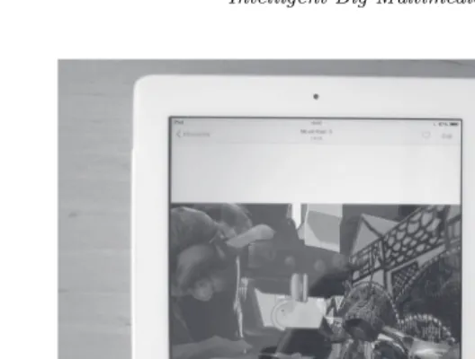
Fig. 1.6 Tablet computer and a smartphone.

are pre-computed and stored. The problem of a rapid exact search of large high-dimensional collections of objects is an important problem with applications in many diﬀerent areas (multimedia, medicine, chemistry, and biology). This problem becomes even more urgent when handling large multimedia databases that cannot be processed by one server but require the processing power hundreds to thousands of servers.

1.3 Guide to the Reader

(24)

representa-Introduction 7

Fig. 1.7 We have a limited understanding of our human brain. An example of an fMRI image indicated row positions of changes of brain activity associated with various stimulus conditions. A cluster indicates a brain activity during an experiment [Wichert et al.(2002)].

tion, such as the wavelet transformation, the scale space, the subspace tree and deep learning.

1.4 Content

Multimedia Databases - Chapter 2 We begin with a short introduc-tion to relaintroduc-tional databases and introduce examples of popular multimedia information. Multimedia data enable new data access methods, such as query by images, in which the most similar image to the presented image is determined, which is also referred to as content-based image retrieval (CBIR).

(25)

Compression - Chapter 4 The size of a multimedia object may be im-mense. For the eﬃcient storage and retrieval of large amounts of data, a clever method for encoding information using fewer bits than the original representation is essential. Two categories of compression exist: lossless compression and lossy compression. Both types of compression reduce the amount of the source information. No information is lost during lossless compression, which is not the case during lossy compression. When com-pressed information is decomcom-pressed in lossy compression, a minor loss of information and quality occurs. This is achieved by the identiﬁcation of unnecessary or unimportant information that can be removed. Lossy com-pression is primarily based on human perceptual features.

Feature Extraction - Chapter 5 The extraction of primitive out of media data is referred to as feature extraction. The set of features represents relevant information about the input data in a certain context. The context is dependent on the desired task, which employs the reduced representation instead of the original input. The set of primitives is usually described by a feature vector. Feature extraction is related to compression algorithms and is frequently based on the transform function described in the previous chapter. During content-based media retrieval, the feature vectors are used to determine the similarity among the media objects. We introduce the basic image features and then describe the scale-invariant feature transform (SIFT). The GIST is a low-dimensional representation of a scene that does not require any segmentation. We highlight the concept of recognition by components (GEONS). Next, we explain the speech formant frequencies and phonemes. A feature vector represents the extracted features that describe multimedia objects. We introduce the distinction between the nearest neighbor similarity and the epsilon similarity. When the features are represented by sequences of varying length, time wrapping is employed to determine the similarity between these features.

(26)

Introduction 9

be constructed. At the end of the chapter, we introduce fractals and the Hausdorﬀ dimension.

Approximative Indexing - Chapter 7 The metric index trees eﬃ-ciently operate with a small number of dimensions. An increase in the number of dimensions has negative implications for the performance of multidimensional index trees. These negative eﬀects, which are referred to as the “curse of dimensionality”, state that any algorithm for high di-mension dandn objects for an exact nearest neighbor must either use an

nd_{-dimension space or have a query time of} _n_×_d _[B¨_ohm _{et al.} _(2001)],

[Pestov (2012)]. In approximate indexing, data points that may be lost at certain distances are distorted. Approximate indexing seems to be free from the curse of dimensionality. We describe the popular locality-sensitive hashing (LSH) algorithm and its relation to Johnson-Lindenstrauss Lemma. We then present product quantization for the approximate nearest neighbor search.

High Dimensional Indexing - Chapter 8 Traditional indexing of mul-timedia data creates a dilemma. Either the number of features has to be reduced or the quality of the results in unsatisfactory or approximate query is preformed, which causes relative error during retrieval. The promise of the recently introduced subspace tree is the logarithmic retrieval complex-ity of extremely high-dimensional features. The subspace tree indicates that the conjecture “the curse of dimensionality” may be false. The search in this structure begins in the subspace with the lowest dimension. In this subspace, the set of all possible similar objects is determined. In the next subspace, additional metric information that corresponds to a higher dimension is used to reduce this set. This process is repeated. The theoret-ical estimation of temporal complexity of the subspace tree is logarithmic for the Gaussian (normal) distribution of the distances between the data points. The algorithm can be easily parallelized for large data. Chunks divide the database; each chunk may be individually processed by ten to thousands of servers.

(27)

document collection can be employed. During information retrieval, the fea-ture vectors are used to determine the similarity between text documents represented by the cosine of the angle between the vectors. Alternative indexing techniques based on random projections are described. We intro-duce an alternative biologically inspired mode “the associative memory” which is an ideal model for the information retrieval task. It is composed of a cluster of units that represent a simple model of a real biological.

Statistical Supervised Machine Learning - Chapter 10 Several par-allels between human learning and machine learning exist. Various tech-niques are inspired from the eﬀorts of psychologists and biologists to simu-late human learning using computational models. Based on the Perceptron, we introduce the back-propagation algorithm and the radial-basis function network; both may be constructed by the support-vector learning algo-rithm. Deep learning models achieve high-level abstraction by architec-tures that are composed of multiple nonlinear transformations. They oﬀer a natural progression from a low level structure to a high level structure as demonstrated by natural complexity. We describe the Map Transformation Cascade (MTC), in which the information is sequentially processed; each layer only processes information after the previous layer is completed. We show that deep learning is intimately related to the subspace tree and pro-vide a possible explanation for the success of deep belief networks and its relation to the subspace tree,

Multimodal Fusion - Chapter 11 A multimodal search enables an information search using search queries in multiple data types, including text and other multimedia formats. The information is described by some feature vectors and categories that were determined by indexing structures or supervised learning algorithms. A feature vector or category can be-long to diﬀerent modalities, such as word, shape, or color. Either late or early fusion can be performed; however, our brain seems to perform a unimodal search with late fusion. Late fusion can be described by the stochastic language model approach and the Dempster-Shafer theory. In the Dempster-Shafer theory, measures of uncertainty can be associated with sets of hypotheses to distinguish between uncertainty and ignorance. The Dempster rule of combination derives common and shared beliefs between multiple sources and disregards all conﬂicting (nonshared) beliefs.

(28)

Introduction 11

collection of unstructured data that cannot be processed with traditional methods, such as standard database management systems. It requires the processing power of hundreds to thousands of servers. To rapidly access big data, divide and conquer methods, which are based on hierarchical struc-tures that can be parallelized, can be employed. Data can be distributed and processed by multiple processing units. Big data is usually processed by a distributed ﬁle-sharing framework for data storage and querying. MapRe-duce provides a parallel processing model and associated implementation to process a vast amount of data. Queries are split and distributed across parallel nodes (servers) and processed in parallel (the Map step).

(29)

b1816_FM.indd vi

b1816_FM.indd vi 10/10/2014 1:12:39 PM10/10/2014 1:12:39 PM

(30)

Chapter 2

Multimedia Databases

We begin with a short introduction to relational databases and introduce examples of popular multimedia information. Multimedia data enables new data access methods, such as query by images, in which the most similar image to the presented image is determined; it is also referred to as content based image retrieval (CBIR).

2.1 Relational Databases

The database evolved over many years from a simple data collection to multimedia databases:

• 1960: Data collections, database creation, information manage-ment systems (IMS) and database managemanage-ment systems (DBMS) were introduced. DBMS is the software that enables a computer to perform the database functions of storing, retrieving, adding, deleting and modifying data.

• 1970: The relational data model and relational database manage-ment systems were introduced by Tedd Codd (1923-2003). He also introduced a special-purpose programming language named Struc-tured Query Language (SQL), which was designed for managing data held in a relational database management system. It is the most successful data model.

• 1980: The introduction of advanced data models were motivated by recent developments in artificial intelligence and programming languages: the object oriented model and the deductive model. Neither of these models gained popularity. They are difficult to model and are not flexible.

(31)

Table 2.1 Employee database with information about employees and the department. Employee and department are entities represented by symbols and the relationships are the links between these entities. A relation is represented by a table of data.

employeeID name job departmentID

9001 Claudia DBA 99

8124 Ana Programmer 101

8223 Antonio Programmer 99

8051 Hans System-Administrator 101

• 1990: Data mining and data warehousing were introduced.

• 2000: Stream data management, global information systems and multimedia databases become popular.

The relational database model is based on relational algebra that is an offshoot of first-order logic and of algebra of sets. Logical representation is motivated by philosophy and mathematics [Kurzweil (1990); Tarski (1995); Luger and Stubblefield (1998)]. Predicates are functions that map objects’ arguments into true or false values. They describe the relation between objects in a world which is represented by symbols. Symbols are used to denote or refer to something other than themselves, namely other things in the world (according to the, pioneering work of Tarski [Tarski (1944, 1956, 1995)]). They are defined by their occurrence in a relation. Symbols are not present in the world; they are the constructs of a human society and simplify the process of representation. Whenever a relation holds with respect to some objects, the corresponding predicate is true when applied to the corresponding objects. A relational database models entities by symbols and relationships between them. Entities are the things in the real world represented by symbols, like for example the information about employees and the department they work for. Employee and department are entities represented by symbols and the relationships are the links between these entities. A relation is represented by a table, see Table 2.1.

Each column or attribute describes the data in each record in the table. Each row in a table represents a record. If there is a functional dependency between columnsAand B in a given table,

A→B,

then, the value of columnAdetermines the value of columnB. In the Table 2.1 employeeIDdetermines the name

(32)

Multimedia Databases 15

A key is a column (or a set of columns) that can be used to identify a row in a table. Diﬀerent possible keys exist; the primary key is used to identify a single row (record) and foreign keys represent links between tables. In the Table, 2.1employeeIDis a primary key anddepartmentIDis a foreign key that indicates links to other tables. A database schema is the structure or design of the database without any data. The employee database schema of Table 2.1 is represented as

employee(employeeID, name, job, departmentID).

A database is usually represented by several tables. During the design of a database, the design ﬂaws are removed by rules that describe what we should and should not do in our table structures. These rules are referred to as the normal forms. They break tables into smaller tables that form a better design. A better design prevents insert anomalies and deletion anomalies. For example, if we delete all employees of department 99, we no longer have any record that indicates that department 99 exists. If we insert data into a ﬂawed table, the correct rows in the database are not distinct. The relational model has been very successful in handling structured data but has been less successful with media data.

2.1.1 Structured Query Language SQL

The role of the Structured Query Language SQL in a relational database is limited to checking the data types of values and comparing using the Boolean logic. The general form is

select a1, a2, ... an from r1, r2, ... rm where P

[order by ....] [group by ...] [having ...]

For example

select name

from student, takes

(33)

Numeric types are called numbers, mathematical operations on numbers are preformed by operators and scalar numerical functions in SQL. Scalar functions perform a calculation, usually based on input values that are provided as arguments, and return a numeric value. For example

select 9 mod 2

9 mod 2 1.

There are no numerical vectors, we can not deﬁne a distance function like

select * from image

where dist(image, given-image) <= 100

and preform similarity search. For example, it is not possible to ﬁnd pairs of branches with similar sales patterns.

2.1.2 Symbolical artiﬁcial intelligence and relational databases

Knowledge representation in symbolical artificial intelligence tries to model the way we humans represent and process knowledge. Of course this rep-resentation is far more complex then the organisational and administrative knowledge representation by relational databases. The relational model could be seen as AI motivated since it is based on the first-order logic. Be-side this, the influence of symbolical AI is mainly marginal and is related to the object-oriented representation and the rule based systems that will be introduced in the next sections. This is not the case with subsymbolical artificial intelligence, it plays an essential part in the domain of data mining and multimedia databases.

2.1.2.1 Semantic nets and frames

(34)

were popularized in computer science by Marvin Minsky. One important result of the frame theory is the object-oriented approach in programming and the object-oriented extensions of SQL. The object-oriented extensions

mammal

is-a animal

gives milk bird

is-a

does lay egg

sing does is-a

nightingale

dolphin

swim is-a

does penguin

is-a

does swim

giraffe

long neck is-a

has

Fig. 2.1 Taxonomic frame representation of some animals.

of SQL:1999 (formerly SQL3) provides the primary basis for supporting object-oriented structures and the deﬁnition of new primitive types, called user-deﬁned primitive types. Related to object-oriented programming lan-guage is the object database. An object database stores complex data and relationships between data directly, the database is integrated with the object-oriented programming language. The programmer can maintain consistency within one environment, this makes it suitable for complex ap-plications. A big disadvantage of this approach is lack of a clear division between the database model and the application.

2.1.2.2 Expert systems

(35)

(1995); Luger and Stubbleﬁeld (1998)] contains several “if” patterns and one or more “then” patterns. A pattern in the context of rules is an in-dividual predicate which can be negated together with arguments. The rule can establish a new fact by the “then” part, the conclusion whenever the “if” part, the premise, is true. When variables become identiﬁed with values they are bound to these values. Whenever the variables in a pattern are replaced by values, the pattern is said to be instantiationed. Here is an example of rules with a variable x:

• If (ﬂies(x)∨feathes(x))∧lays eggs(x)

premise

then bird(x)

conclusion • If bird(x)∧swims(x) then penguin(x)

• If bird(x)∧sings(x) then nightinagle(x)

The following fact are present:

• feathers(Pit)

• lays eggs(Pit)

• swims(Pit)

• ﬂies(Airbus)

(36)

2.2 Media Data

When addressing multimedia in databases, we have to consider digital data representation. We will introduce examples of the most popular multimedia information, namely, text, graphics, digital images, digital audio and digital video.

2.2.1 Text

Text plays the main role in information retrieval (IR). There are four types of text that are used to produce pages of documents;

• unformatted text,

• formatted,

• hypertext,

• text with mark-up language.

Unformatted text is also known as plaintext enables pages to be created which compromise strings of fixed-sized characters from a limited charac-ter set. American Standard Code for Information Incharac-terchange, the ASCII character set, is the most popular code. It was developed based on the English alphabet around 1963. Each character is represented by 7 bits. There are 128 = 27alternative characters, see Figure 2.2. In addition to all normal alphabetic characters, numeric characters and printable characters, the set also includes a number of control characters. The character set was extended to 8 bits by adding additional character definitions after the first 128 characters. The limitation of the ASCII character set was overcome by Unicode [Consortium (2006)]. Unicode is an industry standard that is designed to enable text and symbols from all writing systems of the world to be consistently represented and manipulated by computers. The stan-dard has been implemented in many recent technologies, including XML, the Java programming language, and modern operating systems. Unicode covers almost all current scripts (writing systems), including Arabic, Arme-nian, Thai and Tibetan, as shown in Figure 2.3. Most popular encodings include:

• UTF-8: an 8-bit, variable-width encoding that is compatible with ASCII.

(37)

Fig. 2.2 ASCII table of the ﬁrst 128 characters.

Fig. 2.3 Some example of the Unicode, Latin and Chinese.

Formatted text is used by word processors. It enables pages and com-plete documents, which are composed of strings of characters of diﬀerent styles, size and shapes with tables, graphics, and images inserted at appro-priate points, to be created.

Hypertext enables an integrated set of documents that each comprise formatted text, which have deﬁned linkages created by hyperlinks. Hyper-Text Markup Language (HTML) is an example of a more general set of mark-up languages.

(38)

annotating a document in a manner that is syntactically distinguishable from the text. Examples of mark-up languages include Postscript, TeX, LaTeX, and Standard Generalization Mark-Up Language (SGLM) on which Extensible Markup Language (XML) and HTML are based.

2.2.2 Graphics and digital images

2.2.2.1 Vector graphics

Vector graphics use geometrical primitives, such as points, lines, curves, and polygons, which are based on mathematical equations to represent images in computer graphics. Vector graphics are used in contrast to the term raster graphics (refer to Figure 2.4), which is the representation of images as a collection of pixels (dots) and is related to mark-up languages (refer to Figure 2.5). Consider a circle of radius r. The main pieces of information

Fig. 2.4 A simple raster graphic represented by binary pixels.

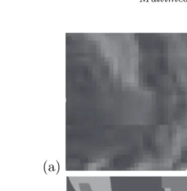
that a program needs to draw this circle are the radius r, the location of the center point of the circle, the stroke line style and color and the fill style and color (possibly transparent). The amount of information translates to a much smaller file size compared with large raster images (refer to Figure 2.6), and the size of representation does not depend on the dimensions of the object. A user can indefinitely zoom in on a circle arc and it remains smooth. In Figure 2.7, an image in a pixel-based representation is converted to a vector graphics representation. In Figure 2.8 (a), we zoom in on the pixel-based image (refer to Figure 2.7); we can recognize the pixels. In Figure 2.8 (b) we zoom in the same area this time in the vector based representation, the regions remains smooth.

2.2.2.2 Raster graphics

(39)

Fig. 2.5 Example of vector graphics.

different colors. The images in the red, green, and blue (RGB) color space consist of colored pixels that are defined by three numbers: one for red, one for green and one for blue (RGB image). The range of different colors that can be produced is dependent on the pixel depth. For a 12 bit pixel depth, four bits per primary color yields

24·24·24= 4096

(40)

Fig. 2.6 Battlezone is an arcade game that was developed by Atari in 1980 using vec-tor graphics. Vecvec-tor graphics were used for some video games in 1980 due to limited computing resources.

2.2.3 Digital audio and video

2.2.3.1 Audio

In signal processing, sampling is the reduction of a continuous signal to a discrete signal. It is the conversion of a sound wave (a continuous time signal) to a sequence of samples (a discrete time signal; refer to Figure 2.10). The sampling frequency or sampling ratefsis deﬁned as the number

of samples obtained in one second; for T seconds,fs is

fs=

1

T

T is referred to as the sample period or sampling interval. The sampling rate is measured in hertz (symbol Hz). Prior to 1960, it was measured in cycles per second (cps). Since 1960, it was oﬃcially replaced by the hertz. The sampling or Nyquist theorem indicates a relation between continuous signalsx(t) in time and discrete signalsx[n], It states that if a functionx(t) in timetcontains no frequencies higher thanM hertz, it can be completely determined by its ordinates for a series of points spaced

1 2·M

seconds apart. With

T= 1

(41)

Fig. 2.7 An image of Sophie Scholl in a pixel-based representation is converted to a vector graphics representation.

T represents the interval between the samples, the samples of functionx(t) are represented asx[n] with

x[n] =x(nT) (2.1)

for all integersn. The double-rate requirement, as speciﬁed by the sampling theorem, is approximately used for signals that represent speech and music. For speech signals, the sampling rate is 50Hz - 10kHz; for stereo signals, this value is multiplied by two. For music-quality audio, the sampling rate is 15Hz - 20kHz; for stereo signals, 2·20 kHz, which is 40 kHz (samples per second). The number of bits per sample must be selected to ensure that the quantization noise generated by the sampling process remains at an acceptable level (reconstructing). In speech, 12 bits per sample are used; in music, 16 bits per sample are used. In most applications that involve music, stereo signals are required and two stereo signals need to be digitized. In practice, a lower sampling rate and fewer bits per sample are utilized.

2.2.3.2 Video

(42)

(a)

[image:42.595.91.279.68.260.2]

(b)

Fig. 2.8 (a) We zoom in on the a pixel-based image (refer to Figure 2.7); we can recognize the pixels. (b) We zoom in on the same area in the vector-based representation; the regions remain smooth.

Fig. 2.9 3D Figure represented by voxels.

[image:42.595.155.262.324.436.2]

(43)

Fig. 2.10 The sound signal “You return safely” spoken during Apollo 13 mission.

(44)

2.2.4 SQL and multimedia

SQL was extended to the use of multimedia for presentational requirements. A sales order processing system can include an online catalog that contains a picture of the oﬀered product. The image can be retrieved via a tradi-tional database record with a key. The extended SQL language is named SQL:1999 (formerly SQL3); it oﬀers two new data types that can store media data [Dunckley (2003)].

• BLOB for binary large objects.

• CLOB for character large objects.

The types are restricted in terms of many SQL operations; for example, for use with comparisons instead of pure equality tests. The manner in which new data types are implemented varies. The media objects can be externally stored as operating system ﬁles or in the database.

• Binary large objects (BLOB) that are locally stored in the database and contain audio, image, or video data or other heterogeneous media data.

• File-based large objects (BFILE) that are locally stored in operat-ing system-specific file systems and contain audio, image, or video data or other heterogeneous media data. A data link enables the SQL to provide a transparent interface for the data that is stored in both the database and the external files.

Because SQL editors cannot cope with the display or input of multimedia in a database, an additional multimedia extender outside the relational database framework is required. The multimedia extender supports popular formats (audio, image, and video data formats) and enables access via traditional and Web interfaces. They also enable querying using media content with optional specialized indexing methods.

2.2.5 Multimedia extender

A multimedia extender is a module outside the relational database model. It is frequently implemented in a programming language, such as Java or

C#. The multimedia extender communicates with the relational database via an interface (for example, JDBC for Java). It extends the reliability, availability, and data management of the database as follows:

(45)

• Access via traditional and Web interfaces.

• Querying using associated relational data.

• Querying using extracted metadata.

• Querying using media content with optional specialized indexing methods. This type of querying is referred to as content-based multimedia retrieval.

2.3 Content-Based Multimedia Retrieval

Traditional text-based multimedia search engines use text-based retrieval methods, which frequently requires manual annotation of multimedia, such as images. An alternative approach is content-based multimedia retrieval. Content-based image retrieval (CBIR) is the most common content-based visual information retrieval application. Other examples include based music retrieval or based video retrieval. Diﬀerent content-based query types, such as exact queries and approximative queries, exists. An exact query can be represented by a predicate that describes the image; for example, we are searching images in which more than half of the image represents the sky,

amount sky >60%.

(46)

Fig. 2.11 The retrieval by a query (example) image.

image retrieval methods, features that describe important properties of im-ages are employed, such as color, texture and shape [Flickneret al.(1995)], [Smeulderset al.(2000)], [Quacket al.(2004)], [Dunckley (2003)].

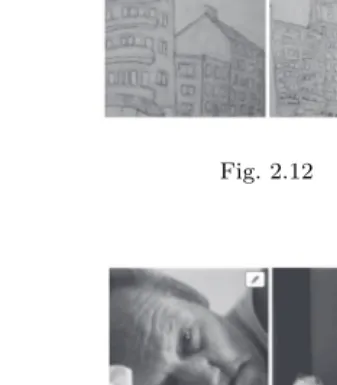
The impact of the features is dependent on the image domain, as demon-strated by two diﬀerent domains of oil paintings (refer to Figure 2.12) and photos (refer to Figure 2.13).

The features that describe the properties of the image are referred to as the image signature. Any query operations solely address the image signature and do not address the image. Using the image signature, a sig-niﬁcant compression is achieved. For a better performance with large image databases, an index for searching the image signatures is constructed. Ev-ery image inserted into the database is analyzed, a compact representation of its content is stored in the signature and the index structure is updated. Traditional data structures are insuﬃcient. The feature extraction mecha-nism and the indexing structure are a part of the multimedia extender.

The best known content-based image retrieval system is the IBM query by image content (QBIC) search system [Niblack et al. (1993)], [Flickner

et al.(1995)]. The IBM QBIC employs features for color, texture and shape,

(47)

[image:47.595.122.291.288.481.2]

Fig. 2.12 Oil paintings.

Fig. 2.13 Some photos.

(48)

indexing and retrieval algorithm with partial sketch image searching capa-bility for large image databases that are based on wavelets. The algorithm characterizes the color variations over the spatial extent of the image in a manner that provides semantically meaningful image comparisons.

2.3.1 Semantic gap and metadata

2.3.1.1 Semantic gap

The majority of the CBIR systems suﬀer from the “semantic gap” problem. Semantic gap is the lack of coincidence between the information that can be extracted from an image and the interpretation of that image [Dunckley (2003)]. The semantic gap exists because an image is usually described by the image signature, which is composed of features such as the color dis-tribution, texture or shape without any additional semantical information. The semantic gap can be overcome by

• image understanding systems,

• manual annotation of the image (metadata).

2.3.1.2 Image understanding

(49)

2.3.1.3 Metadata

The semantic gap can also be overcome by metadata. Metadata can be deﬁned as “data about data”. Metadata addresses the content structure and similarities of data. It can be represented as text using keywords to ensure that traditional text-based search engines can be utilized. The metadata and the original data need to be maintained and we need to know how to store and update the data, which is speciﬁed by multimedia standards.

2.3.1.4 Multimedia standards

Multimedia standards were developed to ensure interoperability and scala-bility. Popular examples are as follows:

• ID3 is a metadata container that is predominantly used in conjunc-tion with the MP3 audio file format. It enables informaconjunc-tion such as the title, artist, album, track number, or other information about the file to be stored in the file1.

• EXIF is a specification for metadata that employs an image file format that is used by digital cameras2. When taking a picture, the digital equipment can automatically embed information such as the date and time or GPS and other camera parameters. Typically, this metadata is directly embedded in the file. Both JPEG and TIFF file formats foresee the possibility of embedding extra information.

• A general example is the Dublin core, which provides substantial ﬂexibility, is easy to learn and ensures interoperability with other schemes [Dunckley (2003)]. The Dublin core metadata can be used to describe the resources of an information system3. They can be located in an external document or loaded into a database, which enables the data to be indexed. The Dublin core metadata can also be included in the web pages within META tags, which are placed within the HEAD elements of an HTML document.

• MPEG-7 is a universal multimedia description standard. It sup-ports abstraction levels for metadata from low-level signal char-acteristics to high-level semantic information. It creates a stan-dardized multimedia description framework and enables

content-1http://id3.org

(50)

based access based on the descriptions of multimedia content and structure using the metadata. MPEG-7 and MPEG-21 are descrip-tion standards for audio, image and video data [Manjunath et al.

(2002)], [Kim et al. (2005)]; however, they do not make any as-sumptions about the internal storage format in a database. The MPEG-21 standard is an extension of the MPEG-7 standard by managing restrictions for digital content usage.

(51)

b1816_FM.indd vi

b1816_FM.indd vi 10/10/2014 1:12:39 PM10/10/2014 1:12:39 PM

(52)

Chapter 3

Transform Functions

Transform functions can be used for lossy and lossless compression; they are the basis of feature extraction and of high dimensional indexing techniques.

3.1 Fourier Transform

It is always possible to translate periodic waveforms into a set of sinusoidal waveforms. Adding together a number of sinusoidal waveforms can approx-imate any periodic waveform. Fourier analysis tells us what particular sets of sinusoids compose a particular complex waveform by mapping the signal from the time domain to the frequency domain.

3.1.1 Continuous Fourier transform

The frequency is the number of occurrences of a repeating event per unit time1. The period is the duration of one cycle of an event and is the reciprocal of the frequency f. For example, if we count 40 events in two seconds, the frequency is

40 2s =

20 1s = 20

1

s = 20hertz

then the period is

T =p= 1 20s.

A repeated event can be a rotation, oscillation, or a periodic wave. For periodic waves, one period corresponds to the time in which a full cycle of

1_{Section 3.1.1 is similar, with some slight changes, to section 9.1, section 3.1.2 is similar}

to section 9.2 and section 3.1.3 is similar to section 9.4 of the book Principles of Quantum Artiﬁcial Intelligence by the same author

(53)

a wave passes. A cycle is represented by the wavelength. The velocity v

of the wave is represented by the wavelength λ divided by the period p. Because the frequencyf is the inverse of the period, we can represent the velocity as

v= λ

p =λ·f (3.1)

and the frequency as

f = 1

T =

1

p = v

λ. (3.2)

If something changes rapidly, then we say that it has a high frequency. If it does not change rapidly, i.e., it changes smoothly, we say that it has a low frequency. The Fourier transform changes a signal from the time domain

x(t) ∈ C to the frequency domain X(f)∈ C. The representation of the signalx(t) in the frequency domainX(f) is the frequency spectrum. This representation has the amplitude or phase plotted versus the frequency. In a wave, the amplitude describes the magnitude of change and the phase describes the fraction of the wave cycle that has elapsed relative to the origin.

The frequency spectrum of a real valued signal is always symmetric; because the symmetric part is exactly a mirror image of the ﬁrst part, the second part is usually not shown.

The complex number X(f) conveys both the amplitude and phase of the frequencyf. The absolute value|X(f)|represents the amplitude of the frequencyf. The phase is represented by the argument ofX(f),arg(X(f)). For a complex number

z=x+i·y=|z| ·ei·θ (3.3)

θ is the phase

θ=arg(z) =tan−1

_y

x

(3.4)

and

|z|=x2+y2 (3.5)

the phase is an angle (radians), and a negative phase corresponds to a positive time delay of the wave. For example, if we shift the cosine function by the angleθ

(54)

Transform Functions 37

the phase of the cosines wave is shifted. It follows as well that

sin(x) = cos(x−π/2). (3.6)

The Fourier transform ofx(t) is

X(f) =

∞

−∞

x(t)·e−2·π·i·t·fdt (3.7)

tstands for time andf for frequency. The signalx(t) is multiplied with an exponential term at some certain frequencyf, and then integrated over all times. The inverse Fourier transform ofX(f) is

x(t) =

∞

−∞

X(f)·e2·π·i·t·fdf. (3.8)

3.1.2 Discrete Fourier transform

The discrete Fourier transform converts discrete time-based or space-based data into the frequency domain. Given a sequence α

αt: [1,2,· · ·, n]→C. (3.9)

The discrete Fourier transform produces a sequence ω:

ωf : [1,2,· · · , n]→C. (3.10)

The discrete Fourier transform of α(t) is

ωf =

1 √ n· n t=1

αt·e−2·π·i·(t−1)· (f−1)

n (3.11)

its wave frequency is (f−_n1) events per sample. The inverse discrete Fourier transform ofωf is

αt=

1 √ n· n f=1

ωf·e2·π·i·(t−1)· (f−1)

n . (3.12)

Discrete Fourier transform (DFT) can be seen as a linear transform F

talking the column vector αto a column vectorω

ω=F·α (3.13)

⎛ ⎜ ⎜ ⎜ ⎝ ω1 ω2 .. . ωn ⎞ ⎟ ⎟ ⎟

(55)

= √1

n· ⎛ ⎜ ⎜ ⎜ ⎜ ⎝

e−2·π·i·(0)·(0)_n _e−2·π·i·(0)·(1)_n _{· · ·} _e−2·π·i·(0)·(n−_n1) e−2·π·i·(1)·(0)_n _e−2·π·i·(1)·(1)_n _{· · ·} _e−2·π·i·(1)·(n−_n1)

..

. ... . .. ...

e−2·π_·i_·(n₋1)·(0)n e−2·π·i·(n−1)· (1)

n · · · e−2·π·i·(n)· (n−1)

n ⎞ ⎟ ⎟ ⎟ ⎟ ⎠· ⎛ ⎜ ⎜ ⎜ ⎝ α1 α2 .. . αn ⎞ ⎟ ⎟ ⎟ ⎠ (3.14) and the inverse discrete Fourier transform (IDFT) can be seen as a linear transformIF talking the column vector ω to a column vectorα

α=IF ·ω (3.15)

⎛ ⎜ ⎜ ⎜ ⎝ α1 α2 .. . αn ⎞ ⎟ ⎟ ⎟ ⎠= 1 √ n· ⎛ ⎜ ⎜ ⎜ ⎜ ⎝

e2·π·i·(0)·(0)

n e2·π·i·(0)· (1)

n · · · e2·π·i·(0)· (n−1)

n

e2·π·i·(1)·(0)

n e2·π·i·(1)· (1)

n · · · e2·π·i·(1)· (n−1)

n

..

. ... . .. ...

e2·π·i·(n−1)·(0)_n _e2·π·i·(n−1)·(1)_n _{· · ·} _e2·π·i·(n)·(n−_n1) ⎞ ⎟ ⎟ ⎟ ⎟ ⎠· ⎛ ⎜ ⎜ ⎜ ⎝ ω1 ω2 .. . ωn ⎞ ⎟ ⎟ ⎟ ⎠. (3.16) Forn= 8

F =√1 8· ⎛ ⎜ ⎜ ⎜ ⎜ ⎜ ⎜ ⎜ ⎜ ⎜ ⎜ ⎜ ⎝

1 1 1 1 1 1 1 1

1e−π·i·1₄ ₋_{i e}−π·i·₄3 ₋₁ _eπ·i·₄3 _i _eπ·i·1₄

1 −i−1 i 1 −i−1 i

1e−π_·i_·₄3 _{i e}₋π_·i_·1₄ ₋₁ _eπ_·i_·1₄ _i _eπ_·i_·3₄

1 −1 1 −1 1 −1 1 −1

1 eπ·i·3₄ ₋_i _eπ·i·1₄ ₋₁_e−π·i·₄1 _{i e}−π·i·3₄

1 i−1 −i 1 i−1 −i

1 eπ_·i_·1₄ _i _eπ_·i_·3₄ ₋₁_e₋π_·i_·3₄ ₋_{i e}₋π_·i_·1₄ ⎞ ⎟ ⎟ ⎟ ⎟ ⎟ ⎟ ⎟ ⎟ ⎟ ⎟ ⎟ ⎠ . (3.17)

The first row of F is the DC average of the amplitude of the input state when measured, the following rows represent the AC (difference) of the input state amplitudes. F can be simplified with

e−π·i·1₄ ₌1_√−i

2 into

F = √1 8 · ⎛ ⎜ ⎜ ⎜ ⎜ ⎜ ⎜ ⎜ ⎜ ⎜ ⎜ ⎜ ⎜ ⎝

1 1 1 1 1 1 1 1

1 1_√−i

2 −i −

1−i

√

2 −1 −

1+i

√

2 i

1+_√i 2

1 −i−1 i 1 −i−1 i

1 −√1−₂i −i 1√−₂i −1 1+√₂i i −√1+₂i

1 −1 1 −1 1 −1 1 −1 1 −√1+₂i −i 1+√₂i −1 1√−₂i i −√1−₂i

1 i−1 −i 1 i−1 −i

1 1+_√i

2 −i −

1+i

√

2 −1 −

1−i

√

2 i

(56)

and represented as a sum of a real and imaginary matrix

F = √1 8 · ⎛ ⎜ ⎜ ⎜ ⎜ ⎜ ⎜ ⎜ ⎜ ⎜ ⎜ ⎜ ⎜ ⎝

1 1 1 1 1 1 1 1

1 √1₂ 0 −√1₂ −1 −√1₂ 0 √1₂

1 0−1 0 1 0−1 0 1 √−1₂ 0 √1₂ −1 √1₂ 0 −√1₂

1−1 1−1 1 −1 1−1 1 √−1

2 0

1

√

2 −1

1

√

2 0 −

1

√

2

1 0−1 0 1 0−1 0 1 √1

2 0 −

1

√

2 −1 −

1 √ 2 0 1 √ 2 ⎞ ⎟ ⎟ ⎟ ⎟ ⎟ ⎟ ⎟ ⎟ ⎟ ⎟ ⎟ ⎟ ⎠ + (3.19)

+√1 8· ⎛ ⎜ ⎜ ⎜ ⎜ ⎜ ⎜ ⎜ ⎜ ⎜ ⎜ ⎜ ⎜ ⎝

0 0 0 0 0 0 0 0 0 √−i₂ −i √−i₂ 0 √i₂ i √i₂

0 −i 0 i0 −i0 i

0 _√−i

2 −i √−i2 0 √i2 i √−i2

0 0 0 0 0 0 0 0 0 _√i

2 −i

i

√

2 0 −

i

√

2 i −

i

√

2

0 i 0 −i0 i0 −i

0 _√i

2 −i

i

√

2 0 −

i

√

2 i −

i √ 2 ⎞ ⎟ ⎟ ⎟ ⎟ ⎟ ⎟ ⎟ ⎟ ⎟ ⎟ ⎟ ⎟ ⎠ . (3.20)

The ﬁrst row measures the DC, the second row the fractional frequency of the amplitude of the input state of 1/8, the third that of 1/4 = 2/8, the fourth that of 3/8, the ﬁfth that of 1/2 = 4/8, the sixth that of 5/8, the seventh that of 3/4 = 6/8 and the eighth that of 7/8 or, equivalently, the fractional frequency of−1/8. The resulting frequency of the amplitude vector ω for a real valued amplitude vector α is symmetric; ω2 = ω6, ω3=ω7andω4=ω8.

3.1.2.1 Example

We generate a list with 256 = 28 elements containing a periodic signalαt

αt=cos

50·t·2· ·π

256

,

see Figure 3.1 (a). The discrete Fourier transform ωf of the real valued

signalαtis symmetric. It shows a strong peak at 50 + 1 and a symmetric

peak at 256−50 + 1 representing the frequency component of the signal

αt(see Figure 3.1 (b)). We add to the periodic signalαtGaussian random

noise from the interval [−0.5,0.5].

α∗_t =cos

50·t·2· ·π

256

(57)

[ht] (a)

(b)

Fig. 3.1 (a) A periodic signalα_t. (b) The discrete Fourier transformω_f.It shows two peaks at 50 + 1 and a symmetric peak at 256−50 + 1.

The represented data looks random, see Figure 3.2 (a). The frequency component of the signalα∗_tare shown in Figure 3.2 (b). A ﬁlter that reduces Gaussian noise based on DFT removes frequencies with low amplitude of

ωf (see Figure 3.3) and performs the inverse discrete Fourier transform.

For dimension reduction of the signal, only a fraction of frequencies with high amplitude are represented.

3.1.3 Fast Fourier transform

(58)

(a)

(b)

Fig. 3.2 (a) A periodic signalα∗_t. (b) The discrete Fourier transformω∗_f.It shows a strong peak at 50 + 1 and a symmetric peak at 256−50 + 1 representing the frequency component of the signalα∗_t. The zero frequency term represents the DC average and appears at position 1 instead of at position 0.

1805. However, because the corresponding article was written in Latin, it did not gain any popularity. The FFT was several times rediscovered, and it was made popular by J. W. Cooley and J. W. Tukey in 1965 [Cooley and Tukey (1965)], [Cormen et al. (2001b)]. The original algorithm is limited to the DFT matrix of the size 2m_×₂m_{, with a power of two. Variants of}

the algorithm for the case in which the size of the matrix is not a power of two exist. The original algorithm decomposesFm recursively.

Fm+1=

1

√

2 ·

Im Dm Im−Dm

·

Fm 0

0 Fm

(59)

(a)

(b)

Fig. 3.3 (a) The discrete Fourier transformω_f∗.(b) A ﬁlter removes frequencies with low amplitude, resulting inω_f.

with the permutation matrixRmgiven thatn= 2m

Rm= ⎛ ⎜ ⎝

r11 · · · r1n

.. . . .. ...

rn1· · · rnn ⎞ ⎟

⎠ (3.22)

with

rab= ⎧ ⎨ ⎩

1 if 2·a−1 =b

1 if 2·a−n=b

0 else

(60)

and the diagonal matrix with n·2 = 2m+1

Dm= ⎛ ⎜ ⎜ ⎜ ⎝

ζ_n0_·₂ 0 · · · 0 0 ζ_n1_·₂· · · 0

..

. ... . .. ... 0 0 · · · ζ_nn_·−₂1

⎞ ⎟ ⎟ ⎟

⎠. (3.24)

For example F2 is decomposed with

D1, ζ4=e−2·π·i·14 →D1=

e−·π·i·0₂ ₀

0 e−·π·i·1₂

=

1 0 0−i

(3.25)

and

R2= ⎛ ⎜ ⎜ ⎝

1 0 0 0 0 0 1 0 0 1 0 0 0 0 0 1

⎞ ⎟ ⎟

⎠ (3.26)

it follows

F2=√1

2·

⎛ ⎜ ⎜ ⎝

1 0 1 0 0 1 0 −i

1 0−1 0 0 1 0 i

⎞ ⎟ ⎟ ⎠·√1₂·

⎛ ⎜ ⎜ ⎝

1 1 0 0 1−1 0 0 0 0 1 1 0 0 1−1

⎞ ⎟ ⎟ ⎠· ⎛ ⎜ ⎜ ⎝

1 0 0 0 0 0 1 0 0 1 0 0 0 0 0 1

⎞ ⎟ ⎟

⎠ (3.27)

F2= 1 2·

⎛ ⎜ ⎜ ⎝

1 1 1 1

1 −i−1 i

1−1 1−1 1 i−1 −i

⎞ ⎟ ⎟

⎠. (3.28)

The complexity of the FFT algorithm that decomposes Fm recursively is O(n·m).

3.1.4 Discrete cosine transform

The discrete Fourier transform of α(t) is

ωf =

1 √ n· n t=1

αt·e−2·π·i·(t−1)· (f−1)

n . (3.29)

Using the Eluer’s formula

(61)

it can be represented as

ωf =

1 √ n· n t=1

αt·(cos

−2·π·(t−1)·(f−1)

n

+

i·sin

−2·π·(t−1)·(f−1)

n

) (3.31)

and

ωf=

1 √ n· n t=1

αt·(cos

2·π·(t−1)·(f−1)

n

−

i·sin

2·π·(t−1)· (f −1)

n

). (3.32)

For a real valued signal, the spectrum is symmetric, so half of the spectrum is redundant. However, for the reconstruction of the signal through the inverse Fourier transform, the real part and the imaginary part are both required. DCT is a Fourier-related transform similar to the discrete Fourier transform (DFT), but it only uses real numbers.

γ_f =√1

n· n

t=1 αt·cos

2·π·(t−1)·(f−1)

n

(3.33)

Due to normalization it is usually deﬁned as

γf =w(t)· n−1

t=0 αt·cos

π· f·(2·t+ 1)

2·n

. (3.34)

with

w(t) =

_√1

n f or t= 0

2 n else

The resulting spectrum is represented by the absolute value of real numbers and is not redundant. Due to normalization, the spectrum is deﬁned over the entire frequency space.

3.1.4.1 Example

We generate a list withn= 256 = 28elements containing a periodic signal

αt,

αt=sin

60·t·2·π

256

.

The discrete Fourier transform ωf. It shows two peaks at 60 + 1 and a