promoting access to White Rose research papers
White Rose Research Online [email protected]
Universities of Leeds, Sheffield and York
http://eprints.whiterose.ac.uk/
This is an author produced version of a conference paper presented at UK e-Science All Hands Meeting 2006
White Rose Research Online URL for this paper:
http://eprints.whiterose.ac.uk/id/eprint/78060
Paper:
Handley, J, Brodlie, KW and Clayton, RH (2006)Model based visualization of cardiac virtual tissue.In: Cox, SJ, (ed.) Proceedings of the UK e-Science All Hands Meeting 2006. UK e-Science All Hands Meeting 2006, 18th-21st September 2006, Nottingham, UK. NeSC , 233 - 240. ISBN 0-9553988-0-0
Model Based Visualization of Cardiac Virtual Tissue
J W Handley∗, K W Brodlie∗, R H Clayton† ∗School of Computing, University of Leeds, Leeds LS2 9JT
†University of Sheffield, Department of Computer Science,
Regent Court, 211 Portobello Street, Sheffield S1 4DP
Abstract
In standard analysis of simulations of the heart, usually only one state variable – the trans-membrane voltage (or action potential) – is visualized. While this is the ‘most important’ vari-able to visualize, all but the most basic cardiac models have many state varivari-ables at each node; data that are not used when visualizing the output. In this paper, we present a novel visualization technique developed within the Integrative Biology project that uses the entire state of the car-diac virtual tissue to produce images based on the deviation from normal propagation of action potential.
1
Introduction
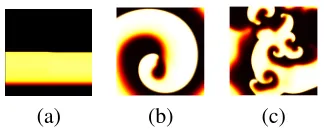
The current generation of high performance computers enable complex simulations of car-diac tissue with anatomically detailed geome-tries [2, 10] — yet the output of these simula-tions are usually visualized using a single out-put from the models; the trans-membrane volt-age, or action potential. This leads to images such as those shown in Figure 1 (see also, for example, [8].) In a normal heartbeat the ac-tion potential propagates from cell to cell as a plane wave across the tissue (Figure 1 (a)), but this propagation can break down into the cir-culating pattern of re-entry (Figures 1 (b) and (c)), a potentially lethal malfunction of heart function. Cardiac arrhythmias such as this are an important cause of premature death in the industrialised world, yet the mechanisms that initiate and sustain the lethal arrhythmias of ventricular fibrillation (VF) and ventricular tachycardia (VT) remain poorly understood.
Experimental and clinical studies of VF mechanisms are limited because it is difficult to record electrical activity throughout the 3D ventricular wall, and so most studies are lim-ited to surface recordings — membrane volt-age can be imvolt-aged on the surface of experi-mental preparations of heart tissue using volt-age sensitive fluorescent dyes. Computational
models, however, allow us to examine the whole tissue, and models of action potential propagation in cardiac tissue (cardiac virtual tissues - CVT) have been used extensively in the last decade to probe the mechanisms of VF [7].
[image:2.596.329.491.435.502.2](a) (b) (c)
Figure 1: Example visualizations of 2D car-diac virtual tissues with (a) normal propa-gation, and re-entrant propagation with (b) one and (c) many re-entrant waves visual-ized using a colourmap where large values are represented by brighter colours.
experimen-tal preparations, but are available in compu-tational models via state variables. Including these variables in visualizations should provide insight into abnormal cardiac function, such as arrhythmias. In this paper we discuss the is-sues of visualizingall the state variables, and present a technique for doing so.
2
Visualizing Cardiac Virtual
Tissue
In the CVT used throughout this paper, action potential propagation is modelled by a reaction diffusion partial differential equation [1]. Sev-eral different excitation models can be used, and these range from simplified models with 3 or 4 state variables, to more detailed models with large nonlinear, stiff systems of ODEs and tens of state variables [6]. The equations are solved across a grid, and typical grid geome-tries are a 2D sheet, a 3D slab, or an anatom-ically detailed representation of the heart ven-tricles.
[image:3.596.321.493.80.280.2]U V W D
Figure 2: A snapshot of re-entry in a 2D model with excitation described by the 4 variable Fenton Karma model [4]. The four state variables are shown individually using the ‘hot’ colourmap where low brightness corresponds to low values.
The visualization challenge can be grasped very quickly through looking at the outputs of two different 2D cardiac virtual tissues. Fig-ure 2 shows a snapshot of the state of a 2D CVT in which a re-entrant wave is rotating. In this model excitability is simulated with the simplified 4 variable Fenton Karma model [4] and in this visualization each state variable is visualized separately. Figure 3 shows a sim-ilar snapshot of a re-entrant wave in a CVT where excitability is modelled using a modifi-cation of the biophysically detailed Luo Rudy
v m h j
d f xs1 xs2
xr b g ato
itto Ca
Figure 3: Snapshot of re-entry in a 2D model with excitation described by the bio-physically detailed Luo Rudy 2 model [3]. As with Figure 2, each state variable is shown individually, except in this model there are 14 state variables.
2 model [3], which has 14 state variables. It is much more difficult to assimilate the 14 im-ages of Figure 3 into a single mental model of the state of the simulation than the four images of Figure 2.
There are many existing techniques for vi-sualizing multi-variate data, such as parallel coordinates, iconic representations or ‘glyphs’, and a review of these and other approaches to the visualization of complex data can be found in [9], however none of these techniques suc-cessfully handle data that are, and need to re-main, four dimensional (i.e. three spatial di-mensions and one temporal) while also being (highly) multi–variate. In this paper, therefore, we concentrate on attempting to reduce the data to an uni–variate space, which can then be visualized easily in four dimensions (using an-imations of isosurfaces, volume rendering, and so on).
Fortunately the dozens of state variables in CVT are not entirely independent, which makes the visualization process easier. This in-terdependence has two main impacts;
may be left out of the visualization, and
2. A collection of state variables can be col-lapsed into a single ‘meta-variable’ which represents the value of all its constituent variables. For example, the parameters
m,h, andjin Figure 3 all depend on mem-brane voltage and time, and determine the magnitude of current through the Na+ channel in the cell membrane, which is needed for an action potential to propa-gate.
The first point can be seen if the correlation co-efficient is calculated between each pair of variables in the four variable Fenton Karma model at each point in time. The correlation used every pixel in a pairwise fashion between each pair of state variables, and can be seen in Figure 4. Note that U and D are almost perfectly correlated across the whole simula-tion, which suggests there would be little extra information gained through including both of these variables in a visualization.
Figure 4: The correlation coefficients of each pair of state variables in the Fenton Karma four variable model across an en-tire simulation. The two letters at the right-hand end of each trace indicate which pair the correlation refers to.
In this paper, we focus on forming visualiza-tions based on every state variable, with the ap-proaches above highlighted as a future refine-ment.
3
Visualizing in Phase Space
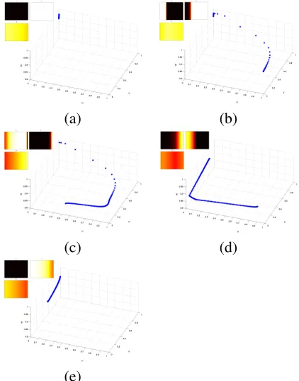
The nature of the propagation of action poten-tial through the heart imposes a structure of sorts on the data, as each cell goes through a
cycle of excitation and recovery. This struc-ture becomes apparent, at least with more sim-ple models, when the data is visualized in phase space. In the case of a tri-variate model, if the standard visualization at time t is to generate threenby m pixel images Ut(x, y),
Vt(x, y), and Wt(x, y), for 0 < x < n
and 0 < y < m, the phase space visual-ization is a single 3D scatter-plot image ob-tained by plotting n×m ‘dots’, one at each
(Ut(x, y), Vt(x, y), Wt(x, y)). Figure 5 shows
examples of phase space plots from a Fenton Karma three variable model exhibiting normal propagation.
(a) (b)
(c) (d)
[image:4.596.312.523.292.561.2](e)
Figure 5: A phase space plot of the 3 param-eters from a 2D Fenton Karma three vari-able model, showing the normal propaga-tion of a wave of acpropaga-tion potential at various intervals. The insets show the false colour images of the three variables. (a) rest state – the points occupy[U = 0, V = 1, W = 1], (b) 30 ms after wave initiation along the left edge of the medium, (c) 90 ms, (d) 150 ms, (e) 210 ms.
[image:4.596.88.284.413.500.2]space. While this ‘snake’ is entirely expected – it occurs as cells depolarise then recover – it nevertheless provides an interesting view on wavefront propagation, and should be present even in higher variate models.
(a) (b)
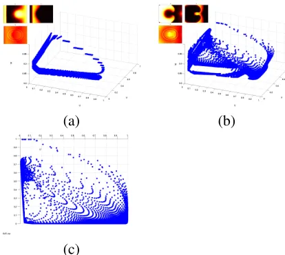
[image:5.596.90.297.164.349.2](c)
Figure 6: A phase space plot of the 3 param-eters from a 2D Fenton Karma three vari-able model, showing re-entrant behaviour. (a) The initiation of the second stimulus — the stimulus that causes re-entry. (b) 145 ms later, when re-entry is well established. (c) A plan view of (b).
Perhaps more interesting effects are ob-served when re-entry is induced in the model. As Figures 6 (b) and (c) shows, the points that previously followed a nominal circumference have now collapsed to almost entirely fill the enclosed space.
Even this simple phase space ‘snake’ pro-vides a novel view of the structure of the model, particularly when re-entrant behaviour is starting or stopping, and it is should be use-ful with higher-variate models through judi-cious choice of the subset of variables plot-ted. It should be noted that adjacent points in real space can be joined in phase space, but we found this cluttered the images without provid-ing any further insight — an intuitive ‘join– the–dots’ interpretation being the correct one.
Clearly the phase space is trivial to visual-ize with two or three variables, but in the case of the Luo Rudy 2 model, with 14 variables, this approach is non-trivial. If the
dimension-ality reduction techniques from section 2 re-duced the phase space even by a factor of three, there would still be too many variables to visu-alize directly. One approach is to create multi-ple phase space plots, which has the advantage that all the data are shown, but the disadvan-tages of still having to visually combine many data sources (see Figure 8, for example). The phase space plots also have the disadvantage of removing spatial information from the visual-ization.
One way forward is to form visualiza-tions based on the density and/or location of the points in the phase space, through ‘hyper-histogram’s [5], but we found this to be a less promising approach than using the propagation-model described in this paper.
4
Propagation-Model Based
Vi-sualization
The phase space ‘snake’ provides an expected behaviour of normal propagation, which in turn suggests the possibility of measuring the deviation from this behaviour. A number of metrics are possible for measuring this devia-tion — in this study we normalised the output from the simulation so that the range of each state variable was[0−1], and then measured deviation as the Euclidean distance to the near-est point in the model. Ideally, the deviation would be measured as the distance from where the simulation pointought to be, but once re-entry is established the concept of the expected state for any given cell becomes meaningless. The nearest ‘normal’ point acts rather as an ap-proximation to where the point would be if all were normal.
in phase-space, at least in part due to the deterministic and quantised simulations being used. Secondly, the computational overhead of performing several hundred thousand distance calculations for every node of the simulation at every point in time would be prohibitive.
[image:6.596.314.499.88.401.2]The decimation was carried about by itetively combining all model points within a ra-diusρof one another into a single point at the mean location of all those points. ρwas cho-sen empirically to be the largest value that vi-sually captured, in phase space, the essence of the model. Note that in this application it is not desirable to decimate by phase-space density, as the model is trying to capture a path through space, not a relative expectation of position in phase-space.
Figure 7 shows the complete and decimated models of normal propagation for the Fen-ton Karma three variable simulation. ρ was
0.02, which reduced the model from 5.4 mil-lion points to 528 points. Clearly the deci-mated model fails to capture the entire region of ‘valid’ phase space; but the essence is cap-tured, and we found the results with this model to be insightful, as described in Section 5.1.
(a) (b)
Figure 7: The model of normal propagation for a Fenton Karma three variable simula-tion. (a) The full model, and (b) the deci-mated model capturing the essence of figure (a).
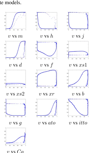
The same process was used for the Luo Rudy 2 simulation, except that a radius of
0.01 was used, resulting in a model of 831 points. The model is partially shown in Fig-ure 8, which displays the model by projecting it onto each of 13 axes formed by the action potential and every other state variable. Note that this figure offers some support for the exis-tence of the phase space ‘snake’ in higher
vari-ate models.
vvsm vvsh vvsj
vvsd vvsf vvsxs1
vvsxs2 vvsxr vvsb
vvsg vvsato vvsitto
[image:6.596.92.292.454.538.2]vvsCa
Figure 8: The model of normal propagation for a Luo Rudy 2 fourteen variable simu-lation. Only a small subset of the model is shown, by plotting the action potential pair-wise with every other state variable. The action potential (v) is on the x-axis in every subplot.
Each data point of CVT is assigned a value based on its Euclidean distance from the near-est point of the propagation model. The result-ing scalar values, in the range[0−√n]for an
n-dimensional model, can be used, at least in this 2-D case to generate false colour images using a standard colourmap.
5
Results and Discussion
(a) (b)
Figure 9: The visualization of the deviation from the model of normal propagation for a normal propagation in the Fenton Karma three variable simulation. (a) The action po-tential output, and (b) the deviation from the model.
As re-entry was introduced in the models, the deviations from the model grew larger, and more interesting images resulted.
5.1 Fenton Karma three variable
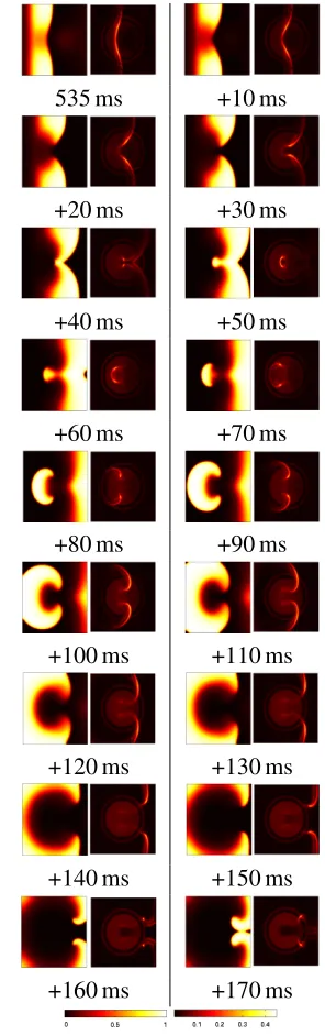
Re-entrant behaviour was introduced in the Fenton Karma three variable simulation by changing the tissue type in the central region such that the recovery following an excitation was delayed. In this way spiral waves are initi-ated when two stimuli are applied in close suc-cession. The onset of re-entry is shown in the sequence of images shown in Figure 10, which are images of the action potential and the devi-ation from the model at 10 ms intervals,
The first feature to note in Figure 10 is that, even when re-entry is well established, nearly all the tissue in the simulation is operating within the expected model for normal propaga-tion, that is it appears dark. The tissue that is deviating from the normal model is very clear at the leading edge of waves of propagation. This is the tissue that has not yet fully recov-ered from an early excitation, and is therefore inhibiting or slowing the propagation of the current excitation. This suggests the combin-ing of the three state variables into a scombin-ingle image is providing an insight into the entire state of the model, in that it becomes possible to predict how the action-potential will propa-gate in the immediate future — something that is not easily assessed from the action-potential images alone. The second feature that can be seen on close inspection of Figure 10 is that the circular heterogeneity in the centre of the do-main has become visible in this visualization, whereas it can not be seen in action potential
images alone.
535 ms +10 ms
+20 ms +30 ms
+40 ms +50 ms
+60 ms +70 ms
+80 ms +90 ms
+100 ms +110 ms
+120 ms +130 ms
+140 ms +150 ms
+160 ms +170 ms
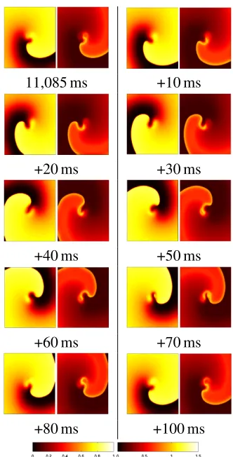
5.2 Luo Rudy 2 fourteen variable
Re-entrant behaviour was introduced in a dif-ferent way for the Luo Rudy 2 simulation — instead of using heterogeneous tissue, the sim-ulation was started in an initial condition where a re-entrant spiral wave immediately forms and continues. The formation of the wave from this artificial start condition was not of interest, so the visualizations were only generated after a settling down period. Figure 11 shows snap-shots at 10 ms intervals of a single revolution of the re-entrant wave, with the action poten-tial and the deviation from the model being dis-played ass before.
The features of this visualization observed in the previous section are present here, in that the re-entrant wavefront shows the largest de-viation from normal, and in particular the tip of the spiral wave. This again represents the regions where propagation is being blocked or delayed. It is interesting to note the very slow drop off of this deviation behind the wave-front – behaviour which contrasts with the very sharp drop-off on the Fenton Karma simula-tion. This may be due a failure of the prop-agation model to capture normal behaviour, or or that this form of re-entry genuinely does dif-fer to this extent from normal propagation. In case, the deviation from the model seems to be far less specific than for the Fenton Karma model.
In these visualizations, the deviation from the model gives a very good impression of the excitation state of any given region of tissue; so much so the action-potential images are not really required in this figure.
6
Conclusions
and
Future
Work
This paper has presented a novel method of visualizing cardiac virtual tissues, through the generation of a model of normal propagation in phase space, and measuring the deviation from this model. In the resulting visualizations, re-gions of CVT where the propagation of ac-tion potential is being delayed are highlighted. When combined with the visualization of
ac-11,085 ms +10 ms
+20 ms +30 ms
+40 ms +50 ms
+60 ms +70 ms
[image:8.596.326.492.81.407.2]+80 ms +100 ms
Figure 11: The visualization of the deviation from the model of normal propagation for re-entrant behaviour in the Luo Rudy 2 sim-ulation. The images show a complete revo-lution of the single spiral wave, with the ac-tion potential on the left, and the deviaac-tion from the model on the right. The colour-bars are shown at the bottom, with the left colour-bar corresponding to the action po-tential images, and the right colour-bar to the deviation images.
tion potential, this provides insight into how the action potential will propagate through the tissue.
normali-sation technique appropriate. There may also be scope in normalising the results between simulations, in that the range of possible dis-tances increases with increasing numbers of state variables.
This visualization technique can be ex-tended to three-dimensional simulations fairly easily. The distance metric is dimension in-dependent, as it is based in phase space. The significant distances occur at the wave-front of action potential, so an interesting visualization might be to form an iso-surface of action po-tential, and colour it according to the deviation from the model.
Acknowledgements
The authors wish to acknowledge the support provided by the funders of the UK e-Science Integrative Biology Project: The EPSRC (ref no: GR/S72023/01) and IBM.
References
[1] R.H. Clayton. Computational models of normal and abnormal action poten-tial propagation in cardiac tissue: Link-ing experimental and clinical cardiology.
Phys. Meas., 22:R15–R34, 2001.
[2] R.H. Clayton and A.V. Holden. Fila-ment behaviour in a computational model of ventricular fibrillation in the canine heart. IEEE Trans. Biomed Eng., 51:28– 34, 2004.
[3] R.H. Clayton and A.V. Holden. Prop-agation of normal beats and re-entry in a computational model of ventricular cardiac tissue with regional differences in action potential shape and duration.
Progress in Biophysics and Molecular Biology, 85:473–499, 2004.
[4] F.H. Fenton, E.M. Cherry, H.M. Hast-ings, and S.J. Evans. Multiple mecha-nisms of spiral wave breakup in a model of cardiac electrical activity. Chaos, 12:852–892, 2002.
[5] J.W. Handley, K.W. Brodlie, and R.H. Clayton. Multi-variate visualization of cardiac virtual tissue. InProc. 19th IEEE International Symposium on Computer Based Medical Systems. IEEE Computer Society, 2006. In press.
[6] D. Noble and Y. Rudy. Models of cardiac ventricular action potentials: Iterative in-teractions between experiment and sim-ulation. Philos. Trans. R. Soc. Lond. Ser. A-Math. Phys. Eng. Sci., 359:1127–1142, 2001.
[7] A.V. Panfilov and A.M. Pertsov. Ven-tricular fibrillation: Evolution of the multiple-wavelet hypothesis. Philos. Trans. R. Soc. Lond. Ser. A-Math. Phys. Eng. Sci., 359:1315–1325, 2001.
[8] Blanca Rodr´ıguez, Brock M. Tice, James C. Eason, Felipe Aguel, Jr. Jos M. Ferrero, and Natalia Trayanova. Ef-fect of acute global ischemia on the up-per limit of vulnerability: a simulation study. Am. J. Physiol. Heart. Circ. Phys-iol., 286(6):H2078–H2088, 2004.
[9] P. Wong and R. Bergeron. 30 years of multidimensional multivariate visualiza-tion. In Gregory M. Nielson, Hans Ha-gan, and Heinrich Muller, editors, Scien-tific Visualization - Overviews, Method-ologies and Techniques., pages 3–33, Los Alamitos, CA., 1997. IEEE Computer Society Press.
![Figure 2: A snapshot of re-entry in a 2Dmodel with excitation described by the 4variable Fenton Karma model [4]](https://thumb-us.123doks.com/thumbv2/123dok_us/8084853.229813/3.596.321.493.80.280/figure-snapshot-dmodel-excitation-described-variable-fenton-karma.webp)