This is a repository copy of
Some remarks on modelling the PDF of the concentration of a
dispersing scalar in turbulence
.
White Rose Research Online URL for this paper:
http://eprints.whiterose.ac.uk/1553/
Article:
Chatwin, P.C. (2002) Some remarks on modelling the PDF of the concentration of a
dispersing scalar in turbulence. European Journal of Applied Mathematics, 13 (1). pp.
95-108. ISSN 0956-7925
https://doi.org/10.1017/S0956792501004727
[email protected] https://eprints.whiterose.ac.uk/ Reuse
Unless indicated otherwise, fulltext items are protected by copyright with all rights reserved. The copyright exception in section 29 of the Copyright, Designs and Patents Act 1988 allows the making of a single copy solely for the purpose of non-commercial research or private study within the limits of fair dealing. The publisher or other rights-holder may allow further reproduction and re-use of this version - refer to the White Rose Research Online record for this item. Where records identify the publisher as the copyright holder, users can verify any specific terms of use on the publisher’s website.
Takedown
If you consider content in White Rose Research Online to be in breach of UK law, please notify us by
DOI: 10.1017/S0956792501004727 Printed in the United Kingdom
Some remarks on modelling the PDF of the
concentration of a dispersing scalar in turbulence
P. C. C H A T W I N
Department of Applied Mathematics, University of Sheffield, Hicks Building, Sheffield S3 7RH, UK
(Received 31 August 2001)
The paper deals with the probability density function (PDF) of the concentration of a scalar within a turbulent flow. Following some comments about the overall structure of the PDF, and its approach to a limit at large times, attention focusses on the so-called small scale mixing term in the evolution equation for the PDF. This represents the effect of molecular diffusion in reducing concentration fluctuations, eventually to zero. Arguments are presented which suggest that this quantity could, in certain circumstances, depend inversely upon the PDF, and a particular example of this leads to a new closure hypothesis. Consequences of this, especially similarity solutions, are explored for the case when the concentration field is statistically homogeneous.
1 Introduction
One of the most important features of turbulent flows is how they disperse scalars (e.g. a dissolved dye, an aerosol in the atmosphere, heat). The concentration of a dispersing scalar (or temperature in the case of heat) is inevitably a random function of position x and timet, but a random function whose statistical properties are determined by physics. Historically research tended to focus on one or two of the simplest statistical properties, especially the (ensemble) mean and variance of the concentration. But, though important, these two properties are not able, in themselves, to provide an adequate (either physical or practical) description of the random concentration field. Thus, there has naturally been increasing focus on other statistical properties including the Probability Density Function (PDF) of concentration.
topic with inadequate understanding, and that there is still considerable scope for simple mathematical models based on good physical insight. The present paper is a contribution with this philosophy.
2 The evolution equation for the PDF
Consider a dispersing scalar in a turbulent flow, subject only to advection and molecular diffusion. More precisely, it will be supposed throughout that the concentrationC(x, t) of the dispersing scalar (or temperature in the case of heat) obeys the advection-diffusion equation
∂C
∂t +U.∇C=κ∇
2C, (2.1)
where U=U(x,t) is the random turbulent velocity field, satisfying mass conservation and the Navier–Stokes equations, and the positive constant κis the molecular diffusivity. The randomness ofUenforces randomness ofC. The PDF ofCis denoted bypC(q;x, t) where (except perhaps at isolated points):
pC(q;x, t) = d dq
prob{C(x, t)6q}
; (2.2)
alternatively,
pC(q;x, t)δq ≈ prob{q6C(x, t)< q+δq}, (2.3)
whereδq is positive and small. SincepC is a PDF, it follows that
Z ∞
0
pC(q;x, t)dq= 1, (2.4)
and the (ensemble) mean concentration E{C}, whereE{·}denotes the expected value, is defined by
E{C}=
Z ∞
0
q pC(q;x, t)dq, (2.5)
with analogous equations for the variance and higher moments – see Mole et al. [18]. The PDF pC(q;x, t) obeys an evolution equation determined from equation (2.1). This equation can be written in many equivalent forms, of which the most convenient for present purposes is
∂pC ∂t +∇.
pC E{U|C =q}
=κ∇2pC−κ
∂2 ∂q2
pC E
(∇C)2 |C=q . (2.6)
3 Some limiting properties of the PDF
In this paper, it is useful to fix attention on a particular type of situation. Suppose that, at t = 0, a finite quantity M of scalar of uniform concentration Cm is released into a turbulent flow in which there is no scalar. This statistically unsteady dispersion situation is a reasonable approximation, at worst, to many real accidents, and was investigated experimentally by Hall et al. [11].
Thus there are regionsΣ1andΣ2, with volumesV1andV2respectively, where the union
of Σ1 andΣ2 is the total regionΣ, with volumeV, available for dispersion, such that
C(x,0) =
(
Cm (x⊂Σ1),
0 (x⊂Σ2).
(3.1)
Note that V and V2 may be infinite. Since subsequent dispersion is governed by
equa-tion (2.1), it follows from a well-known property of this equaequa-tion that, for all times t >0 and for all finite x⊂Σ:
C(x, t)< Cm and C(x, t)>0. (3.2)
Thus there are concentrations q1 =q1(x, t) and q2 =q2(x, t), with q1 >0 and q2 < Cm,
such that
pC(x, t) = 0 for q < q1, q > q2. (3.3)
It merits emphasis that q1 and q2 are determined by the governing equations and by the
choice of ensemble.
Equation (3.2) and its consequence, equation (3.3), arise because equation (2.1) is parabolic, thereby allowing, in effect, some pollutant molecules to have infinite velocities. This is obviously wrong and has led some authors to consider replacing (2.1) by, for example, a generalized telegraph equation (see Monin & Yaglom [19, pp. 676–693]). Nevertheless there is no experimental evidence that (2.1) does not describe turbulent dispersion adequately for all practical purposes, and (3.2) and (3.3) then have to be accepted.
Estimates of the a prioriunknown quantities q1 andq2, and the behaviour of pC near q1 andq2, can in principle be made from data using the statistical theory of extremes –
see Moleet al. [17] and Munroet al. [20] – but there is considerable uncertainty in such estimates.
The constraints in (3.2) and (3.3) have often been overlooked, particularly that q2 is
finite. The latter constraint rules out the power law decay predicted by Sinai & Yakhot [25], the clipped Normal fitted by Mylne & Mason [21] and the clipped gamma derived by Yee & Chan [32], as well as many others.
For the case whenV is finite, the SSMT ensures that the concentration will tend to the uniform value M/V ast→ ∞, i.e.
pC(q;x, t)→δ
q−M V
as t→ ∞. (3.4)
In the limit given by (3.4)
µ=E{C}= M
V ; σ
2=Var
whereVar{.}denotes the variance andσ is the standard deviation ofC. Thus σ
µ →0 as t→ ∞. (3.6)
In view of controversy about the limiting value of σ/µin other circumstances (e.g. see Thomson [29]) it might be worth adding as an aside that whenever it can be deduced thatpC→δ(q−q0) withq0>0,σ/µmust tend to zero. One such example occurs a long
way downwind of a steady source in a windtunnel or pipe of constant cross-section; in this case the limit is approached as downwind distance, rather than time, increases. But in many other cases, such as some pollution plumes, lateral spreading is unconfined so that V in (3.4) is effectively infinite. Then pC →δ(q) so both µ andσ in (3.5) approach zero and (3.6) no longer necessarily holds.
4 The basis of a new closure hypothesis for the SSMT
For the situation described at the beginning of the previous section, the initial structure of pC is given by
pC(q;x,0) =π(x)δ(q−Cm) + [1−π(x)]δ(q), (4.1) whereπ(x) is determined by the selected ensemble. Two examples out of many possibilities
are:
(a) The regionΣ1 has fixed shape and location. Then
π(x) =
(
1 (x⊂Σ1),
0 (x⊂Σ2). (4.2)
Recall thatΣ2 is the complement ofΣ1 within the total regionΣ.
(b) The region Σ is finite with volume V, but the scalar-containing region Σ1 of volume V1 has random shape and location, with the randomness such that
π(x) = V1
V for allx⊂Σ. (4.3)
The condition (4.2) applies to the experiments of Hall et al. [11].
By contrast, when (4.3) holds, pC(q;x,0) is homogeneous, i.e. independent of x. In common with many other studies (e.g. Eswaran & Pope [10] and Jaberi et al. [12]), this paper considers the simplest possible circumstances when pC(q;x, t) is homogeneous for allt. Then equation (2.6) reduces to
∂pC ∂t =−κ
∂2gC
∂q2 , (4.4)
where
gC =pC E
(∇C)2 |C=q . (4.5)
(4.4) and (4.5) could model pC within a box which is continually and randomly stirred with initial conditions given by (4.1) and (4.3).
In summary, therefore, a major problem is to study the way in which pC evolves via (4.4) and (4.5) from the double-delta-function distribution in (4.1) and (4.3) to the single-delta-function distribution in (3.4).
Two distinct types of theoretical method have dominated previous work on this problem. The first, also used in the present paper, is to express the SSMT on the right-hand side of (4.4) in terms, undoubtedly approximate, of pC; this is known as a ‘closure hypothesis’ and has a long history in turbulence, and turbulent dispersion, research beginning with the use of eddy viscosities and diffusivities. Those closure hypotheses that have been applied to the SSMT are discussed by many authors (e.g. Pope [24, pp. 158–163], Borghi [2, pp. 259–261], Kuznetsov & Sabel’nikov [15, pp. 51–53] and Dopazo [9, pp. 409–421]. A popular alternative calculation method for predicting pC is DNS, i.e. equation (2.1) is solved numerically many times sufficient both to (a) include an adequate sample of the possible velocity fields, although the ways in which these are modelled vary greatly, and (b) allow reasonably robust estimations of pC. Papers using DNS include Eswaran & Pope [10], Jaberi et al. [12] and Zimmerman [34]. Use of a closure hypothesis has the great potential advantage over DNS of speed of calculation, but it must be physically reasonable and, for practical use, of known accuracy in specified circumstances.
In laboratory experiments, Tavoularis & Corrsin [27] observed that pC was approxi-mately Gaussian (i.e. a Normal distribution) when there was a constant and non-zero spatial gradient of the mean concentration µ. Pope [24, p. 157] cites this in claiming that an “aim of the modelling is, therefore, to produce Gaussian PDFs whose first and second moments evolve correctly” and later (loc. cit., p. 159) writes “A satisfactory modelled PDF equation should admit this Gaussian PDF as a solution”. In introducing their DNS experiments with spatially homogeneous statistics, Eswaran & Pope [10, p. 515] state that “It is generally assumed that the scalar PDF, starting from a double-delta distribution, evolves towards a Gaussian”, and this claim is repeated by other authors, e.g. Dopazo [9, p. 410]. The following comments may be made immediately:
• The experimental conditions used by Tavoularis & Corrsin [27] are not consistent with an initial double-delta-function distribution.
• A Gaussian PDF, i.e. one for which
pC= 1 σ√2πexp
−(q−µ) 2
2σ2
(−∞< q <∞), (4.6)
where µ = µ(t), σ =σ(t), can at best be an approximation, and an unphysical one, since it does not satisfy (3.3) above.
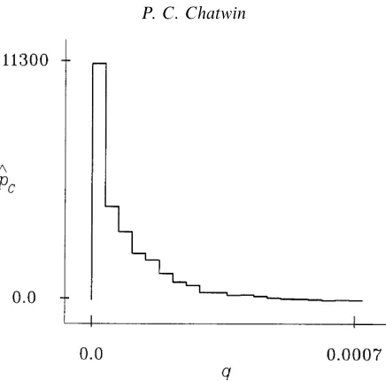
• Measured PDFs in field experiments with an initial double-delta-function distribution are very frequently of the strongly non-Gaussian form typified by Figure 1. (Further examples can be found in Lewis and Chatwin [16] and many other papers.) Character-istic features include a pronounced maximum of pC for a low value of q1 and a long tail which, by (3.3), terminates at a finite value ofq.
Figure 1. Measured values ofpC, denoted by ˆpC, againstqfrom field experiments conducted by Risø National Laboratory, Denmark (BORRIS campaign 1994).
Some evidence for the statement by Eswaran & Pope [10], quoted above, may be found in their paper. Figures 14, 15 and 16 of that paper show that as time evolves the two initial peaks ofpC (used in the simulation to model the initial double-delta-function) shrink in magnitude with a concomitant rise in the values of pC between the peaks. Eventually a single peak, with growing magnitude, emerges. While the final shapes of the graphs of pC against q after four eddy-turnover times appear qualitatively similar to Gaussians, Eswaran & Pope [10, pp. 517–518] note that the flatness (i.e. kurtosis) shows “little sign of levelling off (let alone returning to 3)”, refer to the “lack of Gaussianity of pC”, and state “Thus Figs. 20 and 24 consistently indicate the lack of Gaussianity in pC at the end of the simulations”. However a single simulation for the extended period of twelve eddy-turnover times does suggest that the skewness and kurtosis are approaching the Gaussian values although there is non-negligible statistical variability.
Subsequent to the work of Eswaran & Pope [10], other workers have indeed noted that a Gaussian form ofpC “is only one of many possible outcomes” (Jaberiet al. [12, p. 244]). Later (loc. cit., p. 277) the same authors state that “The primary observation made here is to verify that the long-time PDF of a passive scalar in homogeneous turbulent flows is not necessarily Gaussian (or of any particular form). . . ”. Using a variety of DNS techniques, Jaberi et al. [12] obtain PDFs, some of which are Gaussian and some of which are exponential (the latter, like (4.6), can only be approximate since it too does not satisfy (3.3) above). Kimura and Kraichnan [13] also obtain non-Gaussian PDFs using both DNS and an idealized analytical model.
parameters of the simulations and the initial conditions of the scalar field” (Jaberiet al. [12, p. 241).
The last quote indicates the potential importance of the precise DNS technique used. It also merits emphasis that in the DNS methods used in the papers referred to, in Zimmerman [34], and in many others, periodic boundary conditions were imposed and the resulting PDFs may, at least in part, be influenced by this strong and unreal constraint. Tsinober [31, p. 423] notes that because of periodic boundary conditions: “ . . . the correlation coefficient between two values of any quantity at . . . opposing boundaries, i.e. the points separated at maximal distance in the flow domain, is precisely equal to unity . . . . On the contrary, in any real flow the correlation coefficient becomes very small for points separated by a distance of the order of, and larger than, the integral scale of turbulent flow.”
In summary, the present modelling situation is rather confused, with different numerical techniques giving results that differ strongly from one another in some fundamental respects; nor are they generally consistent with experimental measurements or basic theoretical results like (3.3).
The remainder of the present paper is based on a new idea for closing (4.4). It is claimed merely that this idea may provide fresh insight, not that it will resolve decisively the problems indicated in the previous paragraph.
First, suppose that the initial volume V1 of the scalar-containing region is small
compared with the total volumeV; this is a condition satisfied in nearly all real situations. It has been assumed for many years, following such papers as Batchelor [1] and Corrsin [6], and has relatively recently been directly confirmed in beautiful experiments by Dahm
et al. [7], that scalar-containing regions are drawn out into thin threads or sheets. These become widely separated, and the threads or sheets regenerate (albeit with lower concentrations within them). The thinness ensures large values of |∇C| whereC is large, i.e. E{(∇C)2|C =q}is large when q is large. Since V
1/V is small, large values of q are
associated with small values ofpC as in Figure 1. ThusgC/pC is large wherepC is small, where gC is defined in (4.5). Scalar diffuses by molecular diffusion across the boundaries of these scalar-containing regions into the ambient fluid in which, because V1/V ≪ 1,
concentrations are low and thorough mixing ensures that |∇C|is small there, except very near the boundaries of the thin threads or sheets containing most of the scalar. Thus the converse to the above holds:E{(∇C)2
|C =q}is small whereq is small and, becauseV1/V
is small, small values of q tend to be associated with large values of pC. Thus gC/pC is small where pC is large.
These arguments suggest the qualitative, and new, conclusion that in the postulated circumstances:
pC and gC pC
depend inversely upon one another. (4.7)
This is a principal result in the present paper, arguably the principal result.
It is interesting to compare it with the well-studied proposal in Dopazo (1975), which is that
∂gC
∂q =−
3(ν/κ)
whereλ is the Taylor microscale and ν is the kinematic viscosity. Pope [24, p. 159] and Dopazo [9, p. 411] note that use of (4.8) in (4.4) preserves the shape of pC so that (4.8) does not enable the initial double-delta-function distribution (4.1) to evolve via (4.4) towards, for example, the Gaussian distribution (4.6). While this is a serious drawback, more relevant to present purposes is that, as already noted, both Dopazo and Pope suppose that a closure hypothesis for (4.4) should lead to a pC which is Gaussian. In this case, i.e. when (4.6) holds, it is easy to show that (4.8) gives
gC= 3(ν/κ)
λ2 σ 2p
C, (4.9)
i.e. gC/pC is independent of pC, thus contradicting (4.7).
5 A specific closure hypothesis for the SSMT
This paper has tried to emphasize the difficulty of modellingpC, including the likelihood that many different functional forms occur in practice and therefore that different closure hypotheses for the SSMT may hold in different circumstances. However, a particular closure hypothesis consistent with (4.7) arises from a PDF obtained in earlier work by the author with Zimmerman (Zimmerman & Chatwin [35]; Chatwin & Zimmerman [5]), and it is natural to consider this further. In the first of these papers, turbulent dispersion was modelled simplistically by supposing that the scalar disperses deterministically with no velocity field and the sole stochastic feature is that the sensor measuring C is located randomly within a domain of finite volume. The calculations in the two papers are for a one-dimensional domain−L6x6L, but there is no difficulty in extending the ideas to three dimensions. It is noted that an alternative interpretation of the random feature is that the domain is randomly translated; this is analogous to the random stirring discussed above. The PDF pC can be obtained from first principles by elementary methods. For larget, it is well approximated by
pC(q) = 1
πC0Θ
1−(q−µ) 2
C2 0Θ2
−12
(q1< q < q2), (5.1)
where C0 and µ are positive constants (with µ being the mean concentration as usual),
and
q1=µ−C0Θ , q2=µ+C0Θ , Θ=e−π
2T
, T = κt
l2. (5.2)
This PDF has integrable singularities at q1 and q2, and is symmetric about µ. In view
of the discussion above, it is pertinent to note that as t → ∞ (i.e. T → ∞), q1 → µ
from below and q2 → µ from above. Thus, as t→ ∞, pC in equation (5.1) approaches δ(q−µ) consistent with (3.4). But the approach occurs because the singularities atq1and q2 move closer to one another and eventually coalesce. At no stage is pC approximated, even crudely, by the Normal distribution in (4.6). It may also be noted that it is easy to show from (5.1) that σ =C0Θ/
√
2 so that equation (3.6) is satisfied. Finally, since (5.1) may be rewritten
pC(q) = 1
π(q−q1)
−1 2(q
2−q)−
1 2 (q
it is a member of the beta distribution family which has been used frequently in turbulent dispersion (e.g. see Chatwinet al. [4]).
Now pC in (5.1) must satisfy (4.4) for q1 < q < q2. It is then straightforward to show
from (4.4) that
gCpC= 1
L2 (q1< q < q2). (5.4)
and this is equivalent to
E
(∇C)2 |C=q =gC pC
=
1 pCL
2
(q1< q < q2), (5.5)
consistent with (4.7) above. The results in (5.4) and (5.5) can also be obtained easily and directly from the model equations in Chatwin & Zimmerman [5].
It will also be shown – see (6.17) and the remarks following – that (5.4) applies to an exact solution for the PDF derived and used by Kowe & Chatwin [14].
In both this exact solution, and in (5.1), there are singularities in pC at q =q1 and q =q2, and (5.4) applies in both cases only in the limits as q →q1 from above and as q →q2 from below.
However it is clear that (5.4) cannot apply atq1 andq2 when there are no singularities,
for then bothpC and∇C (hencegC/pC) are zero atq1andq2. Moreover the PDF in (5.1)
is very different in shape from that in Figure 1, and from that underlying the argument leading to (4.7). (It could be argued that each side of the symmetric expression in (5.1) is qualitatively similar to the left-hand side of the experimental curve in Figure 1 so that part of the argument leading to (4.7) still applies.) Thus (5.4) cannot apply universally, but this has nowhere been suggested. Like any other simple closure hypothesis, its range of applicability must be limited and so therefore are the results in the penultimate section of this paper when similarity solutions satisfying (5.4) are briefly investigated.
Before this, it is of interest and importance to consider timescales. From the purely mathematical viewpoint, the lengthLin the Zimmerman & Chatwin [35] model appearing in (5.4) is arbitrary (although the title of the paper makes it clear that it is a microscale in real applications). In the work leading to (5.1), the timescale is of orderL2/κ, whereas
it is well-known that in most circumstances the timescale associated with the evolution of pC is of orderl/u, wherel is proportional to the size of the energy-containing eddies and u is a velocity of the order of the size of the velocity fluctuations. Now [28, p. 67],u3/l is of order ofνu2/λ2 (whereλ is the Taylor microscale introduced in (4.8) and (4.9) above),
so thatl/uis of orderL2/κprovided
L2
κ ∝
λ2
ν ⇒ L∝
λ
(ν/κ)1/2 =λC, (5.6)
where λC is the Taylor microscale of the concentration field [8]. This result is entirely consistent with (4.9) and (5.4). Thus (4.9) gives gCpC ∝ (ν/κ)λ−2(σpC)2 and (5.4) gives gCpC ∝L−2. In general,σpC is of order unity so that themagnitudesof (4.9) and (5.4) are of the same order provided L−2 ∝(ν/κ)λ−2, i.e. L∝λ
6 Some consequences of the new closure hypothesis: similarity solutions
This section shows that the closure hypothesis (5.4) is consistent with two families of similarity solutions for pC. As usual, similarity solutions can be expected to apply in the later stages of the dispersion process when the influence of the initial conditions has weakened. Thus the solutions will not necessarily be expected to satisfy the initial double-delta-function distribution in (4.1), but to have plausibly developed from it in the way, for example, suggested after (5.1) above.
Substitution of (5.4) into (4.4) gives
∂pC
∂t =
κ L2
∂ ∂q
p−C2∂pC
∂q
, (6.1)
which is reminiscent of the porous medium equation
∂u ∂t =∇.(u
n
∇u), (6.2)
except that n is not positive (see Ockendon et al. [22, p. 257]). For similarity solutions, write
T = κt L2 , η=
(q−q0) C0Θ1(T)
, pC = f(η) C0Θ2(T)
, (6.3)
where q0 and C0 are positive constants, and Θ1 , Θ2 and f are positive functions to be
determined. Substitution in equation (6.1) gives
d2 dη2 1 f
= Θ˙2Θ
2 1 Θ3
2
f+Θ˙1Θ1 Θ2
2 ηdf
dη, (6.4)
where a dot denotes differentiation with respect toT. It follows that for similarity solutions there must be constants αandβ such that
˙ Θ2Θ12
Θ3 2
=−α , Θ˙1Θ1 Θ2
2
=−β, (6.5)
where the minus signs are chosen because, then, positive values of α and β allow Θ1
and Θ2 to tend to zero as T → ∞ to attain the limiting delta-function distribution in
equation (3.4). Then equation (6.4) becomes
d2 dη2 1 f
=−αf−βηdf
dη. (6.6)
It follows from equation (6.5) that ˙ Θ2 Θ2 = α β ˙ Θ1 Θ1 , (6.7)
and hence that
Θ2 =AΘ1α/β, (6.8)
whereA is an arbitrary positive constant. Thus
˙
Θ1=−βA2Θ1(2α−β)/β, (6.9)
Ifαβ
Θ1 = h
2(α−β)A2T +Θ10−2(α−β)/βi−β/ 2(α−β)
Θ2 =A h
2(α−β)A2T+Θ10−2(α−β)/βi−α/2(α−β),
(6.10)
where Θ10 = Θ1(0). It follows from equation (6.10) that α > β because, if α < β,
equation (6.10) predicts that Θ1 = Θ2 = 0 in finite time. For large values of T, the
dependence of Θ1 and Θ2 on Θ10 weakens, and the results in equation (6.10) can be
approximated by
Θ1 =2(α−β)A2T−
β/2(α−β)
, Θ2=A2(α−β)A2T−
α/2(α−β)
, (6.11)
or, more concisely,
Θ1 =B1T−p , Θ2=B2T−p−
1
2 , p= β
2(α−β) >0, B2
1 B2 2
= 2(α−β). (6.12)
The second case is whenα=β. Direct integration then gives
Θ1=Θ10e−αA
2T
, Θ2=AΘ10e−αA
2T
, (6.13)
and equation (6.6) becomes
d2 dη2 1 f
=−α d
dη(ηf). (6.14)
Equation (6.14) can be integrated once trivially, and the substitutionηf=g−1then enables
it to be integrated completely. A special case of this family of solutions is equation (5.1) for which
α= 1, q0=µ , A=π, f= (1−η2)−
1
2. (6.15)
Returning now to the general case given by equation (6.6), an exact solution has been found when α= 2β so that, from equation (6.12),
p= 1
2 , Θ1=B1T
−1 2 , Θ
2=B2T−1 , B1 B2
=α12. (6.16)
This solution is
f(η) =dη−1(clogη)−12 (6.17)
forη1< η < η2 wherec=−αd2, andd is an arbitrary positive constant. Thus c <0 and η <1 for the realistic case when α is positive. The expression in equation (6.17) gives a PDF satisfying equation (2.4) provided
log(1/η1)
1 2
−
log(1/η2)
1 2 = 1
2T
−1
2, (6.18)
independently of the values ofαandd. A special case of this exact solution is equation (30) in Chatwin & Zimmerman [5] when
η1= exp
−41T
, η2= 1. (6.19)
distributions in equation (3.4) is again approached by the modes coalescing and not via the Gaussian (Normal) PDF in equation (4.6). As well as arising in the model of Zimmerman & Chatwin [35], it is remarkable to note that essentially the same PDF was shown by Kowe and Chatwin [14] to occur in certain cases when the velocity field is the linear rate-of-strain field considered in a classical paper describing ‘hot spots’ by Townsend [30]. (The random feature is then that the principal axes of rate-of-strain are oriented in random directions in space.)
Solutions of equation (6.6) when α and β have arbitrary values must presumably be found numerically; in all cases there will be an equation analogous to equation (6.18).
There is an interesting generalisation of equation (5.4), the closure hypothesis proposed in this paper and investigated above. This is to replace equation (5.4) by
gCpC= h(T)
L2 , (6.20)
where h(T) is an arbitrary (non-dimensional) function taking positive values. Physically, this could represent random stirring at a time-varying intensity. Use of the variables in equation (6.3) in equation (4.4), but with equation (6.20) replacing equation (5.4), yields
h d 2
dη2
1 f
= Θ˙2Θ
2 1 Θ3
2
f+Θ˙1Θ1 Θ2
2 ηdf
dη, (6.21)
instead of equation (6.4). Thus ˙ Θ2Θ12
Θ3 2
=−αh , Θ˙1Θ1 Θ2
2
=−βh, (6.22)
are the generalisations of the results in equation (6.5). Hence equations (6.6) and (6.8) remain valid without change. Once more there are two cases to consider. Ifαβ
h(T) = 1 2A2(α−β)
d dT
n
Θ1−2(α−β)/βo, (6.23)
whereas, if α=β,
h(T) =−αA12 d
dT {logΘ1}. (6.24)
7 Some concluding remarks
The new closure hypothesis in equation (5.4) has been investigated very recently, using numerical simulations, by Yeun [33] and Zimmerman [34]. Their results are so far preliminary, and do not allow firm conclusions.
As noted near the beginning of this paper, theoretical research on the PDF of a dispersing scalar is still a relatively new topic. While, ultimately, all models must be validated against data, the assumptions made in many papers, and this one, that render the equations to some extent tractable are such that direct experimental comparisons are then not possible. This applies particularly to the simplifications that the scalar distribution and the velocity field are homogeneous. Moreover, costs make experimental investigations of unsteady phenomena in turbulent dispersion unattractive.
physics. But many, if not most, real world processes are also stochastic and it is hoped that this work may encourage applied mathematicians to undertake more stochastic modelling while, at the same time, seeking to understand, and involve, the laws controlling the stochasticity.
Acknowledgements
I thank Alexander Klimenko for helpful conversations and Nils Mole, Ron Smith, Paul Sullivan and Will Zimmerman for helpful comments. I believe that the reviews by the referees of an earlier version of this paper led to significant improvements, and I am grateful to them. Rick Munro has provided invaluable aid. Some of the work described in this paper was done while I was a participant in the Turbulence Workshop at the Isaac Newton Institute for Mathematical Sciences in Cambridge (January–June 1999). The work was partly supported by the CEC (COFIN project: contract number ENV4-CT97-0629).
References
[1] Batchelor, G. K.(1952) The effect of homogeneous turbulence on material lines and surfaces. Proc. Roy. Soc.A213, 349–366.
[2] Borghi, R.(1988) Turbulent combustion modelling.Prog. Energy Combust. Sci.14, 245–292. [3] Chatwin, P. C., Lewis, D. M. & Mole, N.(1996) Atmospheric diffusion: some new
mathe-matical models.Adv. in Comp. Maths.6, 227–242.
[4] Chatwin, P. C., Lewis D. M. & Sullivan, P. J.(1995) Turbulent dispersion and the beta distribution.Environmetrics,6, 395–402.
[5] Chatwin, P. C. & Zimmerman, W. B.(1998) The probability structure associated with a simple model of turbulent dispersion.Environmetrics,9, 131–138.
[6] Corrsin, S.(1959) Outline of some topics in homogeneous turbulent flow.J. Geophys. Res.64, 2134–2150.
[7] Dahm, W. J. A., Southerland, K. B. & Buch, K. A. (1991) Direct, high resolution, four-dimensional measurements of the fine scale structure ofS c≫1 molecular mixing in turbulent flows.Phys. Fluids A,3, 1115–1127.
[8] Dopazo, C.(1975) Probability density function approach for a turbulent axisymmetric heated jet. Centreline evolution.Phys. Fluids,18, 397–404.
[9] Dopazo, C.(1994) Recent developments in pdf methods. In: P. A. Libby and F. A. Williams, editors,Turbulent Reacting Flows, pp. 375–474. Academic Press.
[10] Eswaran, V. & Pope, S. B.(1988) Direct numerical simulations of the turbulent mixing of a passive scalar.Phys. Fluids,31, 506–520.
[11] Hall, D. J., Waters, R. A., Marsland, G. W., Upton, S. L. & Emmott, M. A. (1991) Repeat variability in instantaneously released heavy gas clouds – some wind tunnel exper-iments. Technical Repot LR804(PA), National Energy Technology Centre, AEA Technology, Abingdon, Oxfordshire, UK.
[12] Jaberi, F. A., Miller, R. S., Madnia, C. K. & Givi, P.(1996) Non-Gaussian scalar statistics in homogeneous turbulence.J. Fluid Mech.313, 241–282.
[13] Kimura, Y. & Kraichnan, R. H.(1993) Statistics of an advected passive scalar.Phys. Fluids A,5, 2264–2277.
[14] Kowe, R. & Chatwin, P. C. (1985) Exact solutions for the probability density function of turbulent scalar fields.J. Eng. Maths.19, 217–231.
[16] Lewis, D. M. & Chatwin, P. C.(1997) A three-parameter PDF for the concentration of an atmospheric pollutant.J. Appl. Meteor.36, 1064–1075.
[17] Mole, N., Anderson, C. W., Nadarajah, S. & Wright, C.(1995) A generalized Pareto distri-bution model for high concentrations in short-range atmospheric dispersion.Environmetrics, 6, 595–606.
[18] Mole, N., Chatwin, P. C. & Sullivan, P. J.(1993) Modelling concentration fluctuations in air pollution. In: A. J. Jakeman, M. B. Beck and M. J. McAleer, editors, Modelling Change in Environmental Systems, pp. 317–340. Wiley.
[19] Monin, A. S. & Yaglom, A. M. (1971) In: J. L. Lumley, editor, Statistical Fluid Mechanics, Volume 1. MIT Press.
[20] Munro, R. J., Chatwin, P. C. & Mole, N.(2001) The high concentration tails of the probability density function of a dispersing scalar in the atmosphere.Bound.-Layer Meteor.98, 315–339. [21] Mylne, K. R. & Mason, P. J.(1991) Concentration fluctuation measurements in a dispersing
plume at a range of up to 1000m.Quart. J. Roy. Met. Soc.117, 177–206.
[22] Ockendon, J. R., Howison, S. D., Lacey, A. A. & Movchan, A. B.(1999) Applied Partial Differential Equations. OUP.
[23] Pope, S. B. (1979) The statistical theory of turbulent flames. Phil. Trans. Roy. Soc. A 219, 529–568.
[24] Pope, S. B.(1985) Pdf methods for turbulent reactive flows. Prog. Energy Combust. Sci. 11, 119–192.
[25] Sinai, Ya. G. & Yakhot, V.(1989) Limiting probability distributions of a passive scalar in a random velocity field.Phys. Rev. Lett.63, 1962–1964.
[26] Sullivan, P. J. & Ye, H. (1995) A prognosis for the sudden release of contaminant in an environmental flow.Environmetrics,6, 627–636.
[27] Tavoularis, S. & Corrsin, S.(1981) Experiments in nearly homogeneous turbulent shear flow with a uniform mean temperature gradient. Part 1.J. Fluid Mech.104, 311–347.
[28] Tennekes, H. & Lumley, J. L.(1972)A First Course in Turbulence. MIT Press.
[29] Thomson, D. J.(1990) A stochastic model for the motion of particle pairs in isotropic high-Reynolds-number turbulence, and its application to the problem of concentration variance. J. Fluid Mech.210, 113–153.
[30] Townsend, A. A.(1951) The diffusion of heat spots in isotropic turbulence.Proc. Roy. Soc. A 209, 418–430.
[31] Tsinober, A. (1998) Is concentrated vorticity that important? Eur. J. Mech. B/Fluids, 17, 421–449.
[32] Yee, E. & Chan, R.(1997) A simple model for the probability density function of concentration fluctuations in atmospheric plumes.Atmos. Environment,31, 991–1002.
[33] Yeun, H. K. (2000) An investigation into an idealised model of turbulent dispersion. PhD thesis, University of Sheffield.
[34] Zimmerman, W. B. (2001) Simulations of the probability structure of a dispersing passive scalar.Environmetrics,12, 569–589.