Vortex Method for computing high-Reynolds number flows:
Increased accuracy with a fully mesh-less formulation
Thesis by
Lorena A. Barba
In Partial Fulfillment of the Requirements for the Degree of
Doctor of Philosophy
California Institute of Technology Pasadena, California
2004
c
° 2004
Acknowledgements
It is of course self-evident that this doctoral work would not have been possible without the support of my supervisor, Prof. Anthony Leonard. But in this case, I can confidently say that it applies more than in any other. Prof. Leonard has been thanked by his students for many things: his open-door policy, “access to his wealth of experience and kindness” (I agree), his interest on the student’s work as well as her well-being (indeed!), “great guidance, insight, and patience”, “dedication to research and education” ... it is no wonder that he was recognized as Caltech Mentor of the Year 2000. My indebtedness extends in addition to having been offered a place in GALCIT to become his student, even though he was taking a sabbatical and wasn’t really planning on getting new students that year. And above all, to his continued confidence, trust, and acceptance during all these years.
I am much obliged to the members of my examining committee: Prof. James L. Beck, Prof. Tim Colonius, Prof. Hans Hornung, and Prof. Dale Pullin. To Prof. Colonius in particular, thanks are due for calling to our attention the need to study the importance of convection error. To Prof. Pullin, my gratitude extends to his acceptance of chairing my Candidacy Committee, to the discussions we had of my work and his suggesting the application of the non-symmetric Burgers vortices, and also for showing interest in my well-being and success.
Abstract
For the applications of high Reynolds number flows, the vortex method presents the advantage of being free from numerically dissipative truncation error. In practice, however, many vortex methods introduce some numerical dissipation in mesh-based spatial adaption stages, or schemes such as vortex particle splitting. The need for spatial adaption in vortex methods arises from the Lagrangian framework, which results in an increase of discretization over time. Presently, a vortex method is devised that incorporates radial basis function (RBF) interpolation to provide spatial adaption in a fully mesh-less formulation. Numerical experiments show that there is a potential for higher accuracy in comparison with the standard remeshing techniques. The rate of convergence of the new spatial adaption method is exponential, however convection error limits the vortex method to second order convergence. Avenues for future research involve decreasing convection error, for example by means of deformable basis functions. Nevertheless, the RBF-based spatial adaption scheme has various advantages, in addition to a demonstrated higher accuracy and the obvious benefit of not requiring a regular arrangement of particles or mesh. One presently demonstrated advantage is automatic core size control for the core spreading viscous method, without the need for vortex particle splitting.
Contents
Acknowledgements iii
Abstract iv
1 Introduction and Overview 1
1.1 Basic Formulation of a Vortex Method . . . 3
1.2 Overview . . . 6
2 Contributions to the Vortex Method 14 2.1 Viscous Schemes for Vortex Methods . . . 14
2.1.1 Viscous Splitting . . . 15
2.1.2 Random Vortex Method . . . 18
2.1.3 Deterministic Vortex Methods . . . 19
2.1.4 Particle Strength Exchange . . . 20
2.1.5 Redistribution Method . . . 23
2.1.6 Fishelov Method . . . 25
2.1.7 Diffusion Velocity . . . 26
2.1.8 Core Spreading . . . 30
2.1.9 Least-Squares and Triangulated Vortex Methods . . . 36
2.2 Vortex Blob Discretization and Spatial Adaption . . . 39
2.2.1 Discretization and Vortex Method Initialization . . . 39
2.2.2 Rezoning . . . 41
2.2.3 Beale’s Method of Circulation Processing . . . 42
2.2.4 Remeshing Schemes . . . 43
2.2.5 Vortex Blob Splitting . . . 46
2.3 Introduction and Applications of Radial Basis Functions . . . 48
3.2 Errors of the Blob Discretization . . . 55
3.3 Effects of the Lagrangian Time Evolution . . . 63
3.4 Aspects of Time-Stepping . . . 65
3.5 Experiments Using Standard Remeshing . . . 68
3.6 Experiments with Rezoning and a Higher-Order Cutoff . . . 76
4 Formulation and Testing of Fully Mesh-less Vortex Method 82 4.1 Preliminary Experiments Using SOR . . . 82
4.2 RBF Spatial Adaption Using Iterative Solution Methods . . . 86
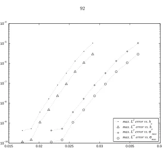
4.3 First Convergence Studies . . . 90
4.4 Practical Considerations of Efficiency . . . 91
4.5 Truly Adaptive Spatial Refinement . . . 93
5 Some Numerical Analysis Topics 95 5.1 Convection Error . . . 95
5.2 Choice of Initial Particle Locations . . . 97
5.3 Analysis of Radial Basis Function Interpolation . . . 103
6 Computations of Viscous Vortex Interactions 106 6.1 Perturbed Monopole with Tripole Attractor . . . 106
6.2 Co-rotating Vortices Before Merging . . . 115
6.3 Non-symmetric Burgers vortices . . . 129
6.4 Observed order of convergence . . . 138
7 Conclusion 143
A Details of Implementation 148
Chapter 1
Introduction and Overview
In this research, a new formulation of the vortex particle method for incompressible flows is imple-mented. The general objective has been to develop improvements in the vortex method to enhance its suitability for the computation of high-Reynolds number flows. To this purpose, the accuracy limitations of the different algorithmic elements of a vortex method have been investigated, with the aim of producing developments in the key components of a code implementation. An additional objective of this investigation is the development of a vortex method that is wholly grid-free, and the demonstration in practice of the capabilities of a grid-free method to accurately compute flows at moderate and high Reynolds numbers.
Vortex methods for the simulation of incompressible flows correspond to a numerical approach with three fundamental features. First, the Navier-Stokes or Euler equations are formulated in terms of vorticity and so the spatial discretization is carried out over the vorticity field instead of the velocity field. Second, making use of one of Helmholtz’ theorems which states the correspondence of vorticity elements with material fluid elements, the computational vortex elements are Lagrangian and so convect with the fluid velocity. And third, to obtain the fluid velocity one makes use of the fact that the vorticity, defined asω=∇×u, can be inverted giving the velocityuas an integral over the vorticity field. This is the Biot-Savart law in vorticity kinematics, which allows to completely describe the flow field by tracking vorticity elements.
satisfying the free-space boundary condition of external flows can be a delicate matter in grid-based methods with truncated flow domains. Furthermore, the Lagrangian vortex particles convect without numerical dissipation, as the non-linear term of the Euler or Navier-Stokes equations is traded by a set of ordinary differential equations for the particle trajectories. This is, again, in contrast with based schemes which inevitably suffer from numerical dissipation. Finally, the essentially grid-free nature of the vortex particle method is itself an advantage, as grid-generation is often one of the most expensive processes in computational fluid dynamics, CFD. The difficulties which arise with vortex methods, on the other hand, will be discussed after first giving a brief historical account.
Vortex methods have been around almost as long as finite differences and the earliest methods of computational mathematics. Indeed, the seminal work of Pr¨ager [160] with vortex distributions on surfaces is the origin of panel methods —widely used in the aeronautics industry to this day, whereas Rosenhead’s work on the calculation of vortex sheets with the point vortex method [169] was of such great consequence that it is still very much cited today; this work is a true classic in the field. Interestingly, Rosenhead’s point vortex method was partially discredited around 1960 by the observation that proof of convergence of the method was lacking [28], and by computer calculations which exhibited apparently chaotic motion of the particles [29]. This last problem was attributed to the singular character of the induced velocity close to a point vortex and different approaches were proposed to deal with it. One of these lead to the vortex blob method [42] which is used in this investigation, while others deal with the problem analytically by removing the singularity in the Biot-Savart expression (see [106, 108, 107]).
The modern vortex method was born in the 1970s and the prominent investigators involved in its early development are A. Chorin, A. Leonard, and C. Rehbach in France. Much interest in vortex methods during the early 1980s focused on mathematical aspects such as the convergence properties [83, 81, 13, 14, 15, 16]. In later years the development of the method was very rich, mainly in relation to the issues of accurate inclusion of viscous effects, the treatment of boundary conditions at solid surfaces, and the efficient reduction of the computational costs, so as to make them suitable for the high-resolution simulation of unsteady, high-Reynolds number flows. Comprehensive reviews of the development of vortex methods and their applications can be found in [113, 114, 197, 183], and [162]; see [5] for a collection of articles that reveal the state of the subject at the beginning of the 1990’s. Recently, a book has been published that is dedicated to the subject including many practical considerations for the implementation of the methods [48].
threefold: (i) the numerical complexity of calculating the velocity using the Biot-Savart law, which is in fact analogous to an “N-body problem” and hence requires orderN2 operations forN vortex
elements; (ii) the inconvenience of adding viscous effects in a Lagrangian formulation, diffusion being viewed as much more readily computed using grid-based methods; and,(iii)the effect of the Lagrangian time evolution, which results on a loss of discretization accuracy due to the distortion of the particle distribution.
The first of the mentioned difficulties has been successfully addressed by the application of the Fast Multipole Method [80] for the calculation of the particle velocities, whereas some workers have bypassed the problem with mixed Eulerian-Lagrangian formulations such as the vortex-in-cell method [43, 55, 175, 45, 196, 30, 64, 119, 118, 54], although at the cost of adding interpolation errors. The inclusion of viscous effects, on the other hand, has benefited from profuse research, there being at least seven proven schemes, with varied degree of success. The loss of accuracy due to Lagrangian distortion of the particles, finally, has been generally dealt with by the application of “remeshing schemes”, which utilize high-order interpolation kernels on a Cartesian tensor product formulation. The standard remeshing schemes have made long-time, accurate calculations of com-plex flows possible; they have, however, caused quite a bit of controversy as they add a mesh to an otherwise mesh-less method. In addition, they do introduce some interpolation error, generally ac-cepted as tolerable. As one wishes to simulate flows at higher Reynolds numbers, however, increased resolution becomes crucial and the interpolation error may be a limitation. Also, a more accurate method may allow for reduced problem sizes at high Reynolds numbers (i.e., smaller numbers of vortex particles for a given accuracy). But most importantly, there are problems in fluid dynam-ics where numerical diffusion, which is introduced inevitably by mesh-based interpolation schemes, can completely annihilate the physics. This is particularly true of vortical flows at high Reynolds numbers. One can cite the example of vortex-blade interaction in rotorblades, where capturing the blade tip vortices for one or more revolutions of the rotor is still impracticable using conventional mesh-based methods [2, 3]. For this reason, the present investigation endeavors to provide a fully mesh-less method of calculation. It is argued that the mesh-less approach can be even extended to spatial adaption processes, and this concept is demonstrated by using a technique of radial basis functions for scattered data interpolation. Ample numerical experimentation will demonstrate that increased accuracy is possible, in comparison with standard vortex methods, and applications in viscous vortex interaction at high Reynolds numbers will thus be practicable.
1.1
Basic Formulation of a Vortex Method
vorticity transport equation is obtained. This is the governing equation in vortex methods, which for three-dimensional flow corresponds to the following vector equation,
∂ω
∂t +u· ∇ω=ω· ∇u+ν∆ω. (1.1)
The assumptions in the above equation are: constant density flow, conservative body forces, an inertial frame of reference and unbounded domain. In the case of a two dimensional and inviscid flow the right-hand side of (1.1) is zero and the governing equation reduces to the simple form
Dω
Dt = 0, where D
Dt stands for the material derivative. This corresponds to the basic formulation of
vortex methods, for which clearly a Lagrangian method based on elements of vorticity is natural and ideal. Based on this simplest of formulations, the vortex method historically found its first successful applications in the simulation of phenomena governed by the 2D Euler equations. Sub-sequently, vortex methods have been extended to three-dimensional flow by including the vortex stretching/tilting term, and have incorporated the presence of internal boundaries by using vortex sheet formulations in the inviscid case and vorticity generation models with boundary elements for the viscous case. Viscous effects were added first by the random walk method [42], but a number of so-called deterministic viscous schemes have been proposed and tested during the last two decades. And recently, some researchers have ventured on the addition of compressibility effects [66, 67, 143]. In the vortex blob discretization, the elements are identified by a position vector, xi; a strength
vector (vorticity×volume) of circulation; and a core size, σi. The discretized vorticity field is
ex-pressed as the sum of the vorticities of the vortex elements in the following way:
ω(x, t)≈ωh(x, t) =
N
X
i=1
Γi(t)ζσi(x−xi(t)), (1.2)
where Γi corresponds to the vector circulation strength of particle i (scalar in 2D). In the blob
version of the vortex method —in contrast to point vortices, the elements have a non-zero core size
σiand a characteristic distribution of vorticityζσi, commonly called the cutoff function. Frequently,
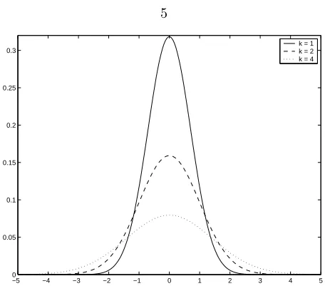
the blob cutoff function is a Gaussian distribution and the core sizes are uniform (σi =σ), which
means that in two dimensions one has
ζσ(x) =
1
kπσ2exp µ
−|x|2
kσ2 ¶
, (1.3)
where the constantkdetermines the width of the cutoff and is chosen by different authors as either 1, 2 or 4. For example, in the review paper of Leonard [113], the Gaussian blob is presented with
−5 −4 −3 −2 −1 0 1 2 3 4 5 0
0.05 0.1 0.15 0.2 0.25
0.3 k = 1k = 2
[image:11.595.209.437.100.304.2]k = 4
Figure 1.1: Gaussian blob distributions, three different versions (1D slice of 2D functions).
In this investigation, we have usedk= 2.
In the majority of vortex methods (almost all), the Lagrangian formulation is expressed by assuming that the vortex elements convect without deformation with the local velocity. The velocity is obtained from the vorticity using the Biot-Savart law:
u(x, t) =
Z
(∇ ×G)(x−x0)ω(x0, t)dx0
=
Z
K(x−x0)ω(x0, t)dx0= (K∗ω)(x, t) (1.4)
where K = ∇ ×Gis known as the Biot-Savart kernel, Gis the Green’s function for the Poisson equation, and ∗ represents convolution. For example, in two dimensions the Biot-Savart law is written explicitly as
u(x, t) = −1
2π
Z (x−x0)×ω(x0, t)ˆk
|x−x0|2 dx
0. (1.5)
For the customary case of an axisymmetric cutoff functionζ=ζ(r),r=|x|, the velocity kernel can be obtained analytically. The velocity regularization function is defined as the integral
q(r) =
Z r
0
ζ(r)r dr. (1.6)
The regularized Biot-Savart kernel is expressed as follows, where×represents cross product (with the vorticity vector, orωˆezin the 2D case) and dis the dimension:
Kσ(x)×=−
q(|x|/σ)
|x|d ·x× (1.7)
Kσ(x) =
1
2πr2(−y, x) µ
1−exp(− r 2
2σ2) ¶
. (1.8)
The formula for the discrete Biot-Savart law in two dimensions gives the velocity as follows,
u(x, t) =−
N
X
j=1
ΓjKσ(x−xj). (1.9)
Finally, the Lagrangian formulation of the (viscous) vortex method in two-dimensions is expressed in the following system of equations:
dxi
dt =u(xi, t) (1.10)
dω
dt =ν∇
2ω + B.C. (1.11)
The complete numerical method is defined by Equations (1.10) and (1.11) which express that the method is to be implemented by integrating the particle trajectories due to the local fluid velocity, while the velocity is obtained from the vorticity using the Biot-Savart law. The vorticity field evolves due to the effects of viscosity, both in the free-stream and on the boundaries (no-slip condition, denoted by B.C.). The viscous effects in the free-stream are enforced by one of a variety of viscosity schemes available for vortex methods (described in §2.1), while the effects due to solid boundaries are traditionally accounted for by generation of vorticity implemented in a version of the boundary element method. This is based on the physical mechanism by which the solid wall is a source of vorticity that enters the flow, so a vorticity flux ∂ω
∂n may be determined at the wall to
satisfy the boundary condition of no-slip at the surface [104].
1.2
Overview
As mentioned, the objective of this research is the development of a vortex method which is capable of computing high-Reynolds number flows accurately. The main difficulty in computing viscous flow at high Reynolds numbers is the fact that numerical diffusion can dominate over the physical viscosity, which many times destroys the physics that one wishes to observe. This is particularly true of viscous flows with concentrated regions of vorticity.
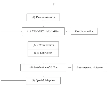
(0) Discretization
(1) Velocity Evaluation
(2a) Convection
(2b) Diffusion
(3) Satisfaction of B.C.’s
(4)Spatial Adaption
-?
?
?
?
Measurement of Forces Fast Summation
[image:13.595.116.531.92.428.2]99K L99
Figure 1.2: Basic building blocks of a viscous vortex method implementation.
and their algorithmic relationships. In small capital letters are indicated the compulsory, minimal components of a viscous vortex method. In slanted font are indicated the parts which, although not obligatory, are generally necessary in a modern application of vortex methods to bounded flows. The arrows designate the program flow in a time-marching algorithm.
The first basic component of a vortex method, the Discretization, consists of representing accurately a given, initial, vorticity field using vortex particles or blobs. This stage includes the choice of a cutoff function and optimal discretization parameters. In essence, as will be discussed amply later on, the problem of accurately discretizing a vorticity field in the vortex method is one of function approximation using nodal functions with global influence. This problem, fortunately, has recently benefitted from considerable research efforts in the function approximation community, and the present work will use their results to remarkable benefit.
The next component in the diagram is the Velocity Evaluation on the location of each vortex element, by use of the discrete Biot-Savart law. Due to the global influence of the vortex particles, calculating the velocity on a single point in space requires O(N) operations, and so the complexity of the direct evaluation of velocity isO(N2). This situation is analogous to the calculation
problem”. Thanks to this analogy, a very important development in vortex methods was due to the cross-over application of the “fast-methods” developed for astrophysics, in particular the Fast Multipole Method (FMM) [80]. These methods have led to the approximate evaluation of velocity with a complexity ofO(NlogN) and evenO(N). Although a production vortex code would almost certainly require a fast summation method for velocity evaluation, particularly in three dimensions, this component has not been incorporated in the present investigation. On the one hand, the solution is well known, and we cannot hope to contribute much in this subject; the application of the FMM in vortex methods is well researched and efficient implementations have been developed [182]. It is, in addition, a component of the implementation that involves great programming effort. On the other hand, the use of a fast Biot-Savart method involves an approximation, and it introduces a controllable error. In this investigation, it is desirable to study the accuracy of all the other components of the vortex method with respect to the direct Biot-Savart evaluation. Subsequently, in a production code with fast velocity evaluation, the error introduced by the fast velocity evaluation is controlled by the multipole acceptance criterion [181], which can be provided as an input parameter to the calculation. Perhaps at the heart of the vortex method are the components labelled (2a) and (2b), i.e.,
ConvectionandDiffusionof the vortex blob elements. The Lagrangian convection of the vortex
particles involves using an adequate time-stepping scheme and choosing an appropriate step size according to the characteristics of the flow and the desired accuracy. These issues will be briefly discussed later, and this investigation will for the most part utilize Runge-Kutta integration schemes of fourth order. Providing viscous diffusion effects, on the other hand, can be quite difficult in the context of a Lagrangian method. Over the past three decades, a vast amount of research in this subject has produced at least seven different schemes for adding viscosity in a vortex method calculation. In more or less chronological order, these are the random vortex method (RVM), core spreading, particle strength exchange (PSE), the vortex redistribution method, diffusion velocity, Fishelov’s method, and the triangulated vortex element method. Due to this profusion of methods, this investigation includes a review and assessment of the advantages and disadvantages of viscous schemes, after which a case is made for the core spreading method. Also, the problems associated with using core spreading will be tackled in a novel (yet simple) way, avoiding numerically diffusive splitting and merging schemes [170, 171].
the particle field on a regular lattice every few time steps, and obtaining the circulation strength at the new particle locations by interpolation or other means. The present investigation will include a considerable amount of numerical experiments and an analysis of the standard methods. In particular, it will be demonstrated that remeshing can introduce visible interpolation errors and can put a limitation on the accuracy of the vortex method. Furthermore, an approach for providing spatial adaption in a mesh-less formulation will be developed and demonstrated, which is based on the technique of radial basis function (RBF) interpolation [31, 32]. This will be the principal contribution of the present research to increasing the accuracy of vortex methods for high-Reynolds number flow computations.
Finally, a vortex method application to bounded flows necessitates theSatisfaction of boundary conditions at the wall. The standard way to provide this, since the introduction of the vortex blob method by Chorin [42], is by application of the concept of vorticity generation at the surface. Implementations for this concept vary, but there is a widespread preference for Neumann-type formulation of the vorticity boundary condition and many workers use a model of vorticity creation at the wall. The vorticity creation algorithm is inspired by the model of Lighthill [116], who invoked the existence of vorticity sources and vorticity sinks in regions of falling or rising pressure (respectively) along a boundary. The prominent approach of formulating a viscous splitting algorithm [46, 104] to satisfy the boundary conditions has led to the popular use of boundary element methods (BEMs) coupled with the vortex method [101, 103, 105, 115, 193, 155, 194, 154, 156]. Although the present investigation has not included a study regarding the accuracy of the standard BEM-vortex method coupling, some ideas have sprouted from the survey of research in the subject of radial basis functions. It is well-known that panel methods “leak”, that is, due to the satisfaction of the boundary conditions at a control point and the use of flat panels to approximate a curved surface, there is a non-zero velocity at the edges of the boundary elements. Since radial basis functions are now also being utilized for accurate three-dimensional geometric modelling [35], it is possible to conceive an application of nodal functions on surfaces to formulate boundary conditions in a vortex method without panels. This, however, is only speculative at the moment and it is proposed as one of the future roads for research.
formulation. Although, as will be seen, hundreds, maybe thousands, of research hours have been spent developing some elaborate algorithms to account for viscous effects, this investigation will be in support of the most utterly simple approach, namely, the core spreading method. It will be argued that the sole problem that rests is the provision of an accurate means for adaptive spatial refinement. Which brings to the next topic in the chapter: the spatial discretization in vortex methods. The way in which an existing or initial vorticity field is discretized using vortex blobs will be discussed first. Then, the different schemes that have been used for providing spatial adaption will be reviewed. It will be seen that all the existing techniques have the shortcoming of introducing a mesh, or rather of being dependent on a regular, Cartesian arrangement of particles. That is, all except for the vortex splitting concept, which nevertheless suffers from numerical dissipation. This discussion will aid in later making the connection between the vortex blob representation and the approximation of functions using nodal bases of global influence, which are briefly introduced at the end of Chapter 2. This, in turn, will lead to formulating applications of the technique of radial basis function interpolation to the initialization of a vortex method calculation and to spatial adaption. These applications will not only allow for a fully grid-free numerical method, but will provide for considerable increase in the accuracy that can be expected from a vortex method computation.
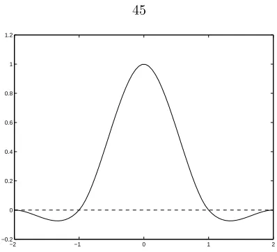
Subsequently, Chapter 3 will present a numerical investigation into the accuracy of vortex meth-ods, including the effects of standard remeshing schemes. To investigate the accuracy of the vortex blob discretization and of the Lagrangian evolution of the vortex particles, two classic test problems are used, both problems of the simplest possible nature: an axisymmetric, inviscid vortex patch (1.12), and a Lamb-Oseen vortex (1.13), given by
ω(r) =
(1−r2)k r61
0 r >1
(1.12)
ω(r, t) = Γ0 4πνtexp
µ
−r
2
4νt ¶
, (1.13)
wherer=x2+y2. The first problem is particularly suited to observe the effects of features in the
inviscid vortex method, as the exact solution consists of circular trajectories of different velocity and the initial particle distribution gets rapidly distorted due to the large shear (hence, this flow belongs to the class of problems known as circular shear layers). This class of problems has been used by many authors to test their methods. The case k= 3 was used for numerical experiments in [16] and it was also used in an example to observe the effect of different particle initializations in [48] (p. 28). Nordmark [144] usedk= 3,7,14 in his numerical experiments and the casek= 7 was also used for accuracy tests by Perlman [152]. In the present work, we have used mostlyk= 3, but
useful to consider different viscosity schemes, being the simplest viscous vortex flow and having an analytical solution; in addition, the vorticity transport equation reduces to the diffusion equation for this problem, so that the viscous effects are decoupled from the nonlinear effects. This classic test problem has been utilized by so many authors, it would be hard to list all of them. Presently, it will be useful in examining the effect of Reynolds number in the loss of regularity of the particle field. It will be seen how for large Reynolds number (small viscosity), the discretization errors quickly grow in a time-marching calculation. This responds to the fact that the vortex particles grow apart in certain areas of the domain, causing gaps to appear and thus becoming unable to reconstruct the smooth vorticity field. This is a well-known problem with vortex methods, which calls for the need to use spatial adaption algorithms.
Using the test problems described above, a study is performed of the errors produced by dis-cretizing the vorticity using vortex blobs, and the importance of the overlap ratio, defined as the inter-particle spacing divided by the core size, h/σ, is clearly demonstrated. The effects of the Lagrangian deformation of the particle field will then be discussed and exposed by numerical exper-iments. Finally, numerical calculations using the standard remeshing schemes will show how these techniques serve to maintain accuracy for long-time simulations, but at the same time introduce noticeable errors themselves.
In addition, Chapter 3 will present numerical experiments exploring the comparative accuracy of different time stepping schemes. This will help to support the use of Runge-Kutta methods, which are sometimes discouraged due to the need for multiple velocity evaluations. In comparison to the one-evaluation Adams-Bashford schemes, it will be shown that the need for a much smaller time step when using Runge-Kutta results in their application being not only more accurate but also more efficient. Finally, this chapter will discuss and present numerical experiments using classic rezoning schemes [16], and demonstrate that they are useful but should only be applied when using high-order blob kernels.
established in the literature on radial basis function interpolation. Some additional discussions will be included regarding the numerical complexity of the evaluation of the RBF interpolants, which can be expensive unless fast methods are used, and regarding the possibilities for truly adaptive spatial refinement that is local, and based on error measurements or estimates.
To follow the presentation and the numerical experiments of the new, mesh-less vortex method formulation, a discussion of some numerical analysis topics in Chapter 5 will clarify some of the possible limitations. A discussion of the effect of a different initial lattice of particle locations will be presented, and an analysis of the convection error. Finally, this chapter includes some topics of numerical analysis of radial basis function interpolation that are likely to be relevant for their application in vortex methods.
In Chapter 6 are presented three applications of significant fluid dynamical interest where the capabilities of the vortex method with mesh-less spatial adaption are tested. The first application consists of the relaxation of monopoles under non-linear perturbations of quadrupolar structure. This flow has previously been shown to possess two possible quasi-steady states, one consisting of a rotating tripole and the other being the axisymmetric state. Which of these “attractors” is approached as the flow relaxes depends on the amplitude of the perturbation. The results obtained here corroborate the existence of this “tripole attractor”, first observed in [174], and also provide smoother and better quality visualization than the previous work. Discrepancy is observed for the low Reynolds number case, which is attributed to the numerical dissipation present in the vortex particle splitting scheme used in [174].
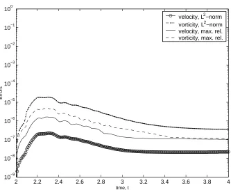
The second application will explore the early interaction of two co-rotating vortices at high-Reynolds number, a problem recently studied by means of spectral methods in [111]. Our calcu-lations are able to reproduce very well the previous results, which constitutes a severe test for the present method. Here, small-scale deformations of the vorticity field are observed in very weak areas, down to a level of 10−6, and we are able to capture these very well. It is also shown that coarser
res-olutions smooth out these small scale deformations and lose some steepness of the vorticity gradient. Significantly, the vortex method is able to reproduce the spectral method results with a problem size reduced by two orders of magnitude. This is attributed to the fact that the vortex method can concentrate computational effort where it is needed, whereas the spectral method requires a very large computational domain to minimize the effects of image vorticity.
In the third and final application, that of non-symmetric Burgers vortices, the core spreading vortex method has needed a correction to account for the out-of-plane strain. This correction has allowed the use of the two-dimensional method for computing flows with uni-directional vorticity and three-dimensional strain, broadening the possible applications for the present method. Results are compared with previously published computations using pseudo-spectral methods [161].
Chapter 2
Contributions to the Vortex
Method
2.1
Viscous Schemes for Vortex Methods
Vortex methods have long proved to be an effective tool for the approximation of solutions to the Euler equations, and have been used for decades in the simulation of both unbounded and bounded flows. In most applications of more than academic interest, however, the limitations of the inviscid approximation cannot be accepted. For example, in flows around solid bodies viscous effects are needed to account for the mechanisms of vorticity generation at the surface and to accurately describe the vorticity dynamics in the wake. Unfortunately, it is not easy to implement a numerical solution of the diffusion term in the vorticity transport equation that is compatible with the Lagrangian formulation. This section examines the different schemes that have been introduced over the years to include viscous effects in vortex methods. First, the viscous splitting algorithm, or fractional step method, is described on which the majority of viscous vortex methods are based. The first scheme that was put forward to account for viscous effects, namely, the random vortex method, is described briefly, since it has become standard practice in engineering applications. The diverse deterministic (as opposed to random or stochastic) viscous schemes that have been introduced during the past twenty years or so as alternatives to the random vortex method include the particle strength exchange method, the redistribution method, Fishelov method, diffusion velocity method, and core spreading method, among others. This diversity of approaches deserves an in-depth analysis, not least because viscosity is a crucial fluid property that can dictate the physics of high-Reynolds number flows.
method). Other methods are not based on viscous splitting but critically depend on the preserva-tion of a certain “order” in the arrangement of vortex elements (e.g., particle strength exchange, Fishelov method) which of course can be a serious problem in a Lagrangian method where elements are bound to become disorganized through convection. Hence, these susceptible methods depend on the application of remeshing processes consisting of tensor product interpolation with high-order kernels. The remeshing processes introduce numerical dissipation due to the interpolations and also do away with one of the favourable features of vortex methods, namely, their grid-free nature. Some methods are intrinsically computationally expensive and make use of manyad hocnumerical param-eters,e.g., the redistribution method, or require further development to be accurate and efficient in the application problems of interest, or are difficult to implement in three dimensions, which could be the case of the redistribution method as well as triangulated vortex elements.
After discussing the features of the different viscous schemes for vortex methods, it will be argued that the simplest of these approaches, core spreading, has the most potential for the applications of high-Reynolds number flows. This method has not been the choice of many workers in vortex methods. First of all, the mathematical objections of Greengard [79] effectively stalled the research efforts using this method, until a solution based on vortex blob splitting was proposed about a decade later by Rossi [170]. The consistency error of core spreading is caused by the advection without deformation of larger and larger vortex blobs as they spread. On the other hand, Rossi’s vortex splitting idea is convergent and effective, but it introduces non-negligible errors. These will be argued here to be caused by numerical diffusion during splitting and lack of any overlap control. In fact, core spreading with vortex splitting may have an accuracy that is no better than the random vortex method. In the present investigation, the core size control needed for convergence of the core spreading method will be implemented without vortex splitting. This contribution will prove to be effectual in making core spreading a suitable method for computing high-Reynolds number flows.
2.1.1
Viscous Splitting
step and first-order overall (irrespective of the time-stepping scheme used). Following [48], this can be realized more easily by looking at the linear convection-diffusion equation for a scalarW,
∂W
∂t +c· ∇W =ν∆W
with initial condition Wo(x). Using operator notation, wherec· ∇ →A andν∆ →B, the above
equation can be written as dWdt =AW +BW, which is integrated to
W(t) =Woe(A+B)t.
Considering discrete time steps of lengthδtthe solution at timenδtis used as initial condition to obtain the solution at the subsequent time step,Wn+1=e(A+B)δtWn. The fractional step method
is then expressed in the following way:
• Sub-step 1: Convection.
dW
dt =AW ⇒ W
n+1
2 =eAδtWn
• Sub-step 2: Diffusion.
dW
dt =BW ⇒ W
n+1=eBδtWn+1
2
• Approximated solution:
Wn+1=eBδteAδtWn
Forδtsmall, the operator in the expression above can be Taylor expanded into
µ
I+δtB+δt
2
2 B
2+
· · ·
¶ µ
I+δtA+δt
2
2 A
2+
· · ·
¶
A comparison with the Taylor expansion of the exact operator e(A+B)δt reveals that the two
expansions are equivalent only in the case of commutivity of the operators A and B. In general, howeverAandB don’t commute, due to the vector fieldcbeing space-dependent, and so the error introduced is O(δt)2 at each time step. Hence, this fractional step method is always first-order
accurate in time.
Temporal accuracy of second order can be achieved with a three-step procedure called “Strang splitting” after [198]. This method is expressed in the following algorithm:
Wn+1=eBδt2eAδteB
δt
2Wn
fractional step method is expressed in the sequence ωn+1 = Hν(δt)E(δt)ωn —where E(t)ω
o and
Hν(t)ω
o are respectively the solutions at time t to the Euler and diffusion equations with initial
conditionωo—. Algorithmically, the method consists in advancing the vortices with the convective
velocity in the first sub-step, and taking account of diffusion in the second sub-step. For two-dimensional, viscous flows
∂ω
∂t +u· ∇ω=ν∆ω. (2.1)
• Sub-step 1: Convection.
∂ω
∂t +u· ∇ω= Dω
Dt = 0
dxp
dt =u(xp)
dωp
dt = 0
(2.2)
• Sub-step 2: Diffusion.
∂ω
∂t =ν∆ω
dxp
dt = 0
dωp
dt =ν∆ω(xp)
(2.3)
The convective sub-step in a vortex method is ideally expressed in the Lagrangian frame of reference, the same as for an inviscid flow. Using the discrete representation of the vorticity field, the velocity is obtained by the Biot-Savart law and the particles are advanced in the inviscid sub-step. But the discretization of the vorticity field in vortex methods, conceived for the simulation of the inviscid vorticity equation, is not well suited for the evaluation of the Laplacian in the diffusive term, because of the unstructured nature of the data. Hence the wide variety of approaches that have been put forward to include diffusive effects in a vortex method, as will be discussed in detail. A straightforward procedure may be to use a grid-dependent scheme such as finite differences to solve the viscous sub-step, and apply mappings of the data from a structured grid overlaid on the irregular particle distribution, as was done in [37], where this method is used to study flow around a circular cylinder at Reynolds numbers of 300–106. This approach partially defeats the
2.1.2
Random Vortex Method
The random vortex method (RVM) was introduced by Chorin [42] and is formulated essentially as a fractional step method. It takes into account the viscous effects in the mean, simulating diffusion by a random walk, i.e., a Brownian-like motion of the vortex particles. Consider the discretized vorticity as expressed by (1.2); in the inviscid case, the particle strengths Γiremain constant, andζ
is not a function of time,i.e., the vortices are elements of fixed geometry, and the particle positions are updated only as a result of convection. Various viscous vortex methods require that either the particle strengths or the base functions be modified in such a way that the diffusion equation is approximately solved. In contrast, the random vortex method acts by modifying the positions of the particles at each (diffusive sub-) step by adding a random walk, that is, the particle locations are transformed using: xni+1=xn
i +ξin, where theξinare Gaussian independent random variables of
zero mean and variance equal to 2ν∆t. This formula is based on the probabilistic interpretation of the diffusion equation, which says that the probability of finding a particle that moves at random in Brownian motion is given by (2.3). Consider the fundamental solution of a one-dimensional diffusion equationωt= Re−1ωxx, for−∞< x <∞, t >0:
G(x, t) =
r
Re 4πtexp
µ
−Re
4tx 2
¶
. (2.4)
The function above is the same as the probability density function of a Gaussian random variable with zero mean and standard deviation σ=√2t/Re. Hence, in two dimensions (2.3) is simulated stochastically by a displacement of the particles in two orthogonal directions, using two independent Gaussian random variables withσ=√2∆t/Re.
The accuracy of the random vortex method was studied in [133], for an initially finite region of vorticity in an unbounded domain. They estimate the error to be of order pν/N, for N vortex particles, which in two dimensions corresponds to first order in the particle spacing,h, for a regular grid. Similarly, the rate of convergence corresponds to orderh3/2in a three-dimensional rectangular
discretization. Convergence proofs for the random vortex method were provided by [120] and [77]. A more detailed description of this method, presentation of convergence analysis and aspects of numerical analysis are provided in [48] (pp. 130–141).
Some benchmark numerical investigations using the RVM can be cited; for example, the circular cylinder flow studies of [175] at Re=250, the simulation of flow around general cylinder shapes at Re=1000 in [195], and circular cylinder flows at Re=3000, 9500 and 104 in [39], and at Re=300,
550, 3000, 9500 in [196]. The RVM has been implemented in parallel [190] taking advantage of the fact that the local nature of the scheme lends itself easily for parallelization. A more recent three-dimensional parallel RVM application to wall bounded flows was presented in [75], where the number of elements used was in the order of 105. Also, many hybrid methods have been introduced
that, based on domain decomposition ideas, utilize the RVM in certain portions of the fluid and either inviscid or other viscous schemes in other zones. For example, in [44] the random walk and diffusion velocity methods were combined for the study of impulsively started flow around a circular cylinder. Diffusion velocity is used near the body surface, while random walk is applied at a certain distance from the body where it is assumed that the noise introduced by the method will not disrupt the boundary layer and affect force calculations. More recently, workers have experimented with a hybrid RVM/Finite volume method as well [157]. Research using the RVM is still active, and further applications include internal flows [76], turbulent flows with flames [36], and flows with free-surface effects [168, 189].
It is safe to say that the RVM has been the most widely utilized of viscous vortex methods, especially in engineering applications. But we wish to quote Prof. Sarpkaya [183] when he says that “the simulation of viscous diffusion by random walk is based on numerical convenience and it has nothing whatever to do with the physical process being simulated.”
2.1.3
Deterministic Vortex Methods
The limited accuracy of the random vortex method motivated the development of deterministic schemes, from the 1980’s onward. Many of these are also based on the viscous splitting concept, while some of the most prevalent are formulated by an integral representation of the solution to the heat equation, and the discretization of the integral operators using the particle positions as quadrature points, as described below.
The solution of the diffusion equation is expressed in integral form as follows,
ω(x, t) =
Z
G(x−y, νt)ω0(y)dy (2.5)
where G represents the heat kernel, i.e., the Green’s function solution of the diffusion equation, which in two dimensions is
G(x−y, τ) = 1 4πτe
−|x−y.|2/4τ (2.6)
a change in the strength of the vortex particles Γi at the diffusion sub-step. The method consists of
resampling the vorticity field induced by each particle on its neighbors, in the following manner. If in the discretized vorticity (1.2), the circulation is replaced by vorticity times volume and the delta function is used as cutoff, and in (2.5) the vorticity at time step tn is used as initial condition to
obtain the vorticity at the next time step due to diffusion, after evaluating at the particle locations the following formula is obtained:
ωnp+1= N
X
q=1
vqωnqG[xpn−xnq, νδt]. (2.7)
This last equation is the induction rule used to update the vorticity of each particle at the diffusion sub-step. However, if used as presented above, the method does not conserve total circulation. To correct it, the fact is used that the heat kernel integrates to 1 over the whole domain, and the vorticity attn+1 is re-written as
ω(x, tn+1) =ω(x, tn) +
Z
G(x−y, νδt)[ω(y, tn)−ω(x, tn)]dy. (2.8)
Again, substituting the discretized form of the vorticity and evaluating at the particle locations, the following conservative scheme is obtained to update the particle vorticities,
ωn+1
p =ωnp +
N
X
q=1
vq(ωnq −ωnp)G[xnp −xnq, νδt]. (2.9)
For more details, see [48]. As explained therein, other resampling methods have been proposed, for example by utilizing another cutoff function instead ofGwhich has the same moment properties. The method of Particle Strength Exchange (PSE) is a generalization of the idea of redistributing the particle circulations, similarly based on the integral approximation of the diffusion equation, but not conceptually linked to viscous splitting. Resampling methods turn out to be a particular case of PSE where a low-order discretization in time is used; hence, PSE, which has been amply tested in high-resolution simulation of moderate to high-Reynolds number flows, is discussed next.
2.1.4
Particle Strength Exchange
∇2ω(x)≈ 2 σ2
Z
ζσ(x−x0) [ω(x0)−ω(x)]dx0 (2.10)
or,
∇2ω(x)≈
Z
Gσ(|x−x0|) [ω(x0)−ω(x)]dx0. (2.11)
The order of accuracy of the approximation above depends on the smoothing function. It is accurate toO(σ2) for the Gaussian, in which case one has
Gσ(x) = 2
πσ2exp Ã
− |x|2
2σ2 !
(2.12)
so that when σ2 = 2νδt, G
σ is equivalent to the heat kernel. The integral operator in (2.11) is
discretized by quadrature, using as quadrature points the locations of the particles. Hence, for the case of bounded flow, one can formulate the PSE method in the following way. The Lagrangian viscous vortex method expressed by Equations (1.10) and (1.11) is translated into the integral formulation
dxp
dt =−
1 2π
Z
K(xp−x0)×ωdx0+Uo(xp, t)
dω
dt = ν
Z
Gσ(|x−x0|) [ω(x0)−ω(x)]dx0
+ν Z
H(xp,x0)
∂ω ∂n(x
0)dx0
where the second term on the right-hand side of the second equation is the contribution from vorticity generation at the surface; Uo contains the contribution from the free stream velocity and any solid
body rotation, and K(z) = z/|z|2. Note that the mechanism of vorticity generation at the solid surface is expressed by an integral operator also, but this topic will not be discussed further here.
The full discretized equations can now be written. Using ωh(x, t) =P
iΓi(t)ζσ(x−xi(t)), the
following system is obtained,
dxp
dt =−
1 2π
X
i
ΓiKσ(xp−xi) +Uo(xp, t) (2.13)
dΓp
dt =ν
N
X
i=1
[Γi−Γp]Gσ(|x−x0|) +ν M
X
m=1
H(xp,xm)
∂ω
∂n(xm) (2.14)
Note that it is assumed that the solid surface was discretized usingM panel elements. Both singular integral operators were convolved with the smoothing function and are replaced by smooth operators;
Kσ is the regularized Biot-Savart kernel,Kσ=K∗ζσ.
splitting is as follows,
1. Particles are advanced using the velocity computed by the Biot-Savart law and integrated using an appropriate time-stepping scheme; their strength is modified using PSE, and the no-through flow boundary condition is enforced. At the end of this sub-step there is a slip velocity at the solid boundary.
2. The no-slip boundary condition is enforced by a vorticity generation algorithm. The vorticity flux from the surface within the time step is calculated so as to cancel the slip velocity generated at the previous sub-step.
In summary, the main feature of the PSE method is the replacement of differential operators by integral operators, more suited to the particle representation of the data. The integral operators are discretized by quadrature on the locations of the particles, then the discrete integral operator for diffusion reduces to a contribution from nearby particles to a change of circulation on a given vortex blob. Note that in Equation (2.14) the strength exchange is written as involving all particles; in practice, though, each vortex particle is allowed contributions to the change in its circulation strength from particles within a radius of, say, 5σ (as in [155]). This is allowed by the rapidly decaying smoothing function; it does mean that the discrete PSE operator does not approximate exactly the continuous integral, and so sometimes a re-normalization of the PSE kernel becomes necessary.
Let us conclude by saying that the PSE method has been extensively developed and applied in many benchmark problems of bluff-body flow. For example, high-resolution simulation of the impulsively started cylinder at Reynolds number from 40 to 9500 in [101, 103], and impulsively started and uniformly accelerated flat plate in [105]. The method has also been implemented in parallel [182] and applied to flows around arbitrary geometries [155]. For this reason, whereas the RVM can be considered the workhorse vortex method used in engineering, PSE can be considered the prevalent vortex method used by the academic community.
2.1.5
Redistribution Method
The motivation for the development of the vortex redistribution method (VRM) was precisely that of providing an alternative to PSE that does away with the need to perform remeshing of the particle field; in other words, the aim was retaining the grid-free formulation of the vortex methods [192]. Similarly to PSE, this method is based on the exchange of circulation between particles to simulate diffusion, but the formulation is different from PSE as it does not use integral operators. The algorithm hinges on finding fractions of each particle’s circulation that will be redistributed among its neighbors, these being defined as those particles within a maximum distance in the order of the typical diffusion distance,hν=
√
ν∆t. The ‘redistribution fractions’fn
ij are solved for by assembling
a system of equations which is formulated so that locally there is conservation of circulation, linear and angular momentum. The following transformation is sought:
ωn =X
i
Γniζσ(x−xi)−→ωn+1=
X
i
X
j
fijnΓniζσ(x−xj). (2.15)
The approach used to determine the redistribution fractions is to demand that all finite wave numbers of the Fourier transform be correctly damped. The Fourier transform of the new vorticity field is
b
ωn+1=ζb(kσ)X
i
Γni exp(−ik·xi)
X
j
fijnexp(−ik·(xj−xi)), (2.16)
while the Fourier transform of the exactly diffused vorticity is
c
ωen+1=ζb(kσ)
X
i
Γni exp(−ik·xi) exp(−k2ν∆t). (2.17)
These two Fourier transforms cannot be equal for all values ofk using a finite number of vortices. Using the fact that within a “neighbourhood” of vortex i the distance |xj−xi| ∼
√
∆t is small, the trailing exponentials in the two Fourier transforms can be approximated by a truncated Taylor series. The resulting equations are the redistribution equations, below. The neighbourhood of a particle is taken as a distance in the order of the typical diffusion distance, hν =
√
empirically (in [192],R=√12). Defining the scaled relative vortex position as: ξij ≡x√jν−∆xti (≤R).
The redistribution equations are
O(1) : X
j
fijn = 1 (2.18)
O(√∆t) : X
j
fijnξ1ij= 0;
X
j
fijnξ2ij= 0 (2.19)
O(∆t) : X
j
fijnξ21ij= 2;
X
j
fijnξ22ij= 2;
X
j
fijnξ1ijξ2ij = 0 (2.20)
O(√∆t3) : X
j
fijnξ31ij= 0;
X
j
fijnξ21ijξ2ij= 0;
X
j
fijnξ32ij= 0;
X
j
fijnξ1ijξ22ij= 0. (2.21)
O(√∆tm) : higher-order moment equations, m= 4· · ·M+ 1.
The first three redistribution equations are necessary to ensure consistency in the sense that the numerical solution approximate theO(∆t) diffusive changes in the exact solution, with a truncation error of orderhν. The physical meaning of the equations is the following: (2.18) implies conservation
of circulation for each vortex; (2.19) locally conserves the center of vorticity; and, (2.20) implies the correct expansion of the mean diameter of the vortex system. The subsequent equations can be used to obtain a higher order of accuracy. However, viscous splitting error is present.
Additional components of the scheme are, first, that positivity of the solution is enforced as a stability condition,i.e., it is demanded that all fractions be positive: fn
ij ≥0. The positivity condition
expresses the physical fact that reverse vorticity cannot form spontaneously in the flow field. Second, whenever it is encountered that there is no acceptable solution to the system of equations, an ad hoc algorithm is used that inserts new vortex particles within the neighbourhood in question. The number of vortices can increase without apparent bound when the Reynolds number is high, so vortex particle merging is sometimes used to alleviate this problem. Finally, preconditioning of the system of equations is needed in practice.
The authors of the VRM claim that the advantage of the method is that it retains the grid-free nature of vortex methods, because it is not needed that the particles be in an ordered distribution (in contrast to PSE). This is achieved, however, at the high cost of solvingN underdetermined systems for N particles, at each time step. The size of these systems is determined by the redistribution influence neighbourhood, |xj−xi| ≤R
√
The method also has the disadvantages of using various parameters that need to be “tuned” in a practical implementation, and involving a considerable computational cost, which can be of the same order as the velocity evaluation, and even larger. In comparison, as reported in [48] (p. 163), the computation of diffusion using PSE including remeshing has a small (∼2%) computational cost compared to the convective step.
2.1.6
Fishelov Method
A deterministic scheme for diffusion which is not based on the exchange of circulation was proposed by Fishelov [70], whose suggestion was to convolve the vorticity with a cutoff function and then approximate the second-order derivatives in the Laplacian by explicit differentiation of the cutoff function. The concept is based on Anderson and Greengard [4], who explicitly differentiate the smooth kernel to obtain the stretching term in a three-dimensional inviscid vortex method algorithm. The problem is how to approximate the spatial derivatives appearing in the vorticity transport equation. Assume a uniform grid at t=0, with grid spacing h, and write xhp(t), ωh
p(t) for the
approximate particle locations and approximate vorticity respectively, then using the discretized form of (1.4) one can write
dxhp(t)
dt =
N
X
j=1
Kσ(xhp(t)−xhj(t))ωjh(t)h2, (2.22)
where Kσ is the regularized Biot-Savart kernel, Kσ =K∗ζσ. Then, by explicit differentiation of
the smoothed kernel in Eulerian coordinates, the stretching term can be written as
ωhp(t) N
X
j=1
∇Kσ(xhp(t)−xjh(t))ωhj(t)h2. (2.23)
Similarly for the viscous term, when the vorticity is convolved with the smoothing function,
ω ≈ ζσ ∗ω, then the Laplacian can be approximated in this way: ∆ω ≈ ∆(ζσ ∗ω) = ∆ζσ∗ω.
Approximating the integrals by the trapezoid rule, the following ODE’s are obtained, which together with (2.22) constitute Fishelov’s vortex method, expressed by the following system of equations:
dωp(t)
dt =ω
h p(t)
N
X
j=1
∇Kσ(xhp(t)−xhj(t))ωhj(t)h2
+ν
N
X
j=1
∆ζσ(xhp(t)−xjh(t))ωjh(t)h2. (2.24)
exponentials—, she carries out some simple numerical experiments in two dimensions, using two test problems: a step function initial vorticity, which she compares to RVM results; and Chorin’s periodic test case (from [41]), which has an exact solution.
In [71], Fishelov utilized her method for the simulation of flow around a sphere at Re=3000, where the vortex method was used only in the far-away region and a boundary layer formulation was used near the body with random walks to approximate viscosity. The results presented, however, seem quite coarse and the simulation short-lived. The method was also used by Bernard for two-dimensional turbulent boundary layer flow in [25]. He used vortex sheet elements of rectangular geometry or “tiles” of vorticity, which are convected as solid bodies. The application problems are start-up channel flow at Re=1000 and zero-pressure gradient (Blasius) and stagnation (Faulkner-Skan) boundary layers at Re=1000. These simulations utilize small numbers of elements (N ∼103)
and boundary layer approximations to evaluate the velocity field. Also, an approximate method is used for evaluating the Laplacian of the cutoff function taking advantage of the regular geometry of the vortex elements, and manyad hoc considerations are included for ensuring that no voids in the element population arise as a result of convection, as these would distort the diffusive process.
Applications of the Fishelov method seem to be scarce and have not provided much confidence in it. The method encounters difficulties when the particle field gets distorted, and seems to be even more sensitive to this problem than the PSE scheme. There do not appear to be any ongoing research efforts to use the method with frequent remeshing processes, but in this case PSE may be preferable. However, in the context of analyzing the use of higher-order cutoff functions, the Fishelov method is used in [145] to calculate unbounded two-dimensional vortex flows, using what is called an “automatic rezoning strategy”; this consists in resetting the particle locations on a uniform grid when the error in vorticity has grown past a certain limit. The rezoning scheme was previously introduced for inviscid flows in [144]. This work has not been extended to flows with boundaries; indeed, in [145] it is argued that the use of vorticity creation at the boundary to approximate boundary conditions introduces errors that make the use of high order vortex methods ineffectual.
Finally, as noted in [48] (p. 147), the Fishelov method is not conservative, as it does not include the correction term −ωpPqvq∆ζσ(xp −xq) that the integral approach requires, just as in the
resampling methods,cf.(2.9). This could be rectified, but there does not seem to be further research in this line.
2.1.7
Diffusion Velocity
∂F
∂t +
∂uF
∂x +
∂vF
∂y = 0. (2.25)
The two-dimensional vorticity transport equation (2.1) can be written in this form, using the in-compressibility condition,
∂ω
∂t +
∂ ∂x
·µ
u−ων∂ω∂x
¶ ω
¸
+ ∂
∂y ·µ
v−νω∂ω∂y
¶ ω
¸
= 0. (2.26)
Comparing (2.25) with (2.26), where (u, v) is the convective velocity, the diffusion velocity is defined by the extra contribution to the total velocity, as follows,
ud=−
ν ω
µ∂ω
∂x, ∂ω ∂y
¶
. (2.27)
So that now the vorticity equation can be written in a conservation form as
∂ω
∂t +∇(ωu+ωud) = 0. (2.28)
The concept of a diffusion velocity implies that the net flow of vorticity is proportional to the vorticity gradient, which is analogous to Fick’s First Law of diffusion whereν/ωis taken as a non-constant diffusion coefficient. It translates into saying thatωhas a preferred direction of transport, namely that of ∇ω. The way the vorticity gradient is obtained in the diffusion velocity method is by directly taking the derivatives of the cutoff function in the discretized vorticity representation.
The suitability of the diffusion velocity concept was demonstrated in [146] for a one-dimensional diffusion test problem and for the case of a circular cylinder at Re=1200 and Re=40 (below the limit of applicability of the RVM). However, the results presented for cylinder flow are of rather low resolution when compared with finite-difference calculations (The authors themselves admit: “the streamlines by our method are somewhat clumsy...”). One notes, as well, that the one-dimensional proof-of-concept calculation was started with core sizeσ = 0.4h, which means that overlap of the vortex particles was not enforced.
and results produced using finite differences. One should rightly be apprehensive, however, of the authors’ decision to use thestrengthof the particular vortex particle whose diffusion velocity is being calculated, rather than the local vorticity, in the denominator of Equation (2.27). The authors simply say that the quality of results was “unaffected” by this decision. In addition, to avoid problems were particles are very weak, resulting in very large diffusion velocity, the vortices that are weaker than 0.1% of the maximum circulation are simply deleted.
Additional results for the circular cylinder using the diffusion velocity scheme, but for a wider range of Reynolds numbers in the range of 10−1− −107, were presented in [147]. Although these
calculations are performed over relatively long times, the unsteady forces are rather noisy and the streamline patterns quite rough. Still, enough simulations were performed to present a plot of the change of drag coefficient with Reynolds number, which shows a “good resemblance to that of the experimental data”, according to the authors. One must question, however, results of two-dimensional calculations that claim good agreement with experimental data atRe up to 107, as it
is well-known that there exist considerable three-dimensional effects from aroundRe = 300 up. If one attentively examines the plots presented in [147], one sees qualitative agreement at best.
The diffusion velocity scheme was demonstrated for calculation of thin boundary layers in [199], where a fix was provided for the problem that can present itself where the vorticity is zero while the gradient of vorticity is not (which risks a division by zero). Also, a “bi-zonal” approach is used to solve the topological problem which exists when using vortex blobs near a wall, consisting of using stream-wise elongated elements in the wall region and blobs in the outer region. The method was benchmarked using the flow of an infinite plate moving at constant velocity, an impulsively started plate (Stokes’ 1st problem), a sinusoidally moving plate (Stokes’ 2ndproblem), and a Blasius
boundary layer. Reynolds numbers are in the order of 105 and good agreement with analytical
solutions is reported. Later, the diffusion of an initially square patch of vorticity and flow around a wedge were added to the test cases [200]. These authors formulate the diffusion velocity concept a little differently, starting from the definition of circulation around a curve which encloses surfaceS
Γ =
Z
S
ω·nˆdS. (2.29)
Defining ˜uto be the velocity of the area occupied by vorticity, they take the time derivative of the above equation to obtain
dΓ
dt =
Z
S
· ∂ω
∂t + (˜u· ∇)ω+ω(∇ ·u˜)−(ω· ∇)˜u ¸
·nˆdS= 0, (2.30)
which is true when the integrand is zero:
∂ω
Let ˜u=u+ud, whereuis the fluid velocity andud is the diffusion velocity, and subtract the
three-dimensional vorticity transport equation (1.1) from (2.31), to obtain the following governing equation for the diffusion velocity:
(ud· ∇)ω+ω(∇ ·ud)−(ω· ∇)ud =−ν∆ω. (2.32)
Using the solenoidal property of the vorticity and some vector identities, the above equation is written in the following form, where the diffusion velocity appears once,
−∇ ×(ud×ω) =ν∇ ×(∇ ×ω). (2.33)
The above equation implies
ud×ω=−ν∇ ×ω+∇φ. (2.34)
The gradient of the arbitrary scalar field, ∇φ, can be shown to be equal to zero. At this point the authors of [199] restrict themselves to two dimensions and obtain the definition of diffusion velocity as expressed by (2.27). They add a further simplification by assuming a thin layer where the diffusion in the direction tangential to the wall can be neglected. But the presentation of the diffusion velocity in this way aids in the extension of the scheme to three dimensions.
The extension of the diffusion velocity concept to three-dimensional flows is introduced in [165], and applied to the evolution of an axisymmetric vortex ring with a small periodic perturbation. Since the vorticity transport equation in 3D is a vector equation, the concept of viscous rotation needs to be added to the viscous velocity. These authors decompose the vorticity field in two parts, denoted byωt andωn, which are defined locally at pointx◦ by
ωt(x) =
ω(x)·ω(x◦)
|ω(x◦)|2 ω(x◦), (2.35)
ωn(x) =ω(x)−ωt(x). (2.36)
The decomposition above is used to express the diffusion term ν∆ωin two parts:
ν∆ω=ν(∆ωt+ ∆ωn). (2.37)
account this decomposition, the vorticity transport equation may be written in the following form:
∂ω
∂t +∇ ·(u⊗ω)−(ω· ∇)u=ν(∆ωt+ ∆ωn)
=−∇ ·(ud⊗ω) +ωd×ω
(2.38)
where: ud=−ν
(∇ ⊗ω)·ω
|ω|2
and, ωd=−ν
∆ωn×ω
|ω|2
. (2.39)
Now the vorticity transport equation can be written in the following form:
∂ω
∂t +∇((u+ud)⊗ω)−(ω· ∇)u−ωd×ω= 0. (2.40)
This form of the Navier-Stokes equation is now a nonlinear advection equation,i.e., the diffusion effect was written as a convection term just like in the two-dimensional diffusion velocity method. The first two terms are interpreted as a convective derivative, the third term is still vortex stretch-ing/tilting, and the last term expresses a rotation applied to the vorticity field. At this point, the Lagrangian particle discretization can be applied and the problem is translated into a set of ordinary differential equations. The Lagrangian system is
dxp
dt =up+ud (2.41)
dωp
dt = (ωp· ∇)up−ωd×ωp. (2.42)
The diffusion velocity in the above system is obtained by a discrete form of equations (2.39), using the discrete vorticity field (1.2) and approximating the term∇ ×ωby
∇ ×ω(x)≈X
i
Γi× ∇ζσ(xi−x). (2.43)
Finally, the calculation of thediffusion vorticityor viscous rotationωdrequires the approximation
of the Laplacian ∆ωn, for which the authors of [165] propose the direct discretization of the integral
approximation, as used in the PSE method for the complete diffusion operator.
Investigations into the use and extension of the diffusion velocity concept continue and are plentiful, including a specific method for axisymmetric flows [164], application to Fokker-Planck equations [117], and an extension of the method to the case of anisotropic diffusion [22].