Non linear Site Response Analysis of Soil Sites in Northern Thailand during the M_w 6 8 Tarlay Earthquake

Article

Non-linear Site Response Analysis of Soil Sites in

Northern Thailand during the M

w

6.8 Tarlay

Earthquake

Lindung Zalbuin Mase

_{, Suched Likitlersuang}

_{, and Tetsuo Tobita}

1 Geotechnical Research Unit, Department of Civil Engineering, Faculty of Engineering, Chulalongkorn

University, Bangkok, Thailand

2 Department of Civil Engineering, Faculty of Engineering, University of Bengkulu, Bengkulu, Indonesia

3 Department of Civil, Environmental, and Applied System Engineering, Kansai University, Japan

E-mail: a_{lmase@unib.ac.id (Corresponding author),} b_{fceslk@eng.chula.ac.th,} c_{tobita@kansai-u.ac.th}

Abstract. On 24 March 2011, the 6.8 Mw Tarlay Earthquake occurred at the border of

Thailand and Myanmar. The earthquake not only resulted in structural building damage but also triggered liquefactions on sandy soils in Northern Thailand. Several site investigations including SPT and shear wave velocity measurements are conducted to study subsoils condition in this area. Ground motions at several seismic stations were recorded during the earthquake. In this study, four soil sites in Chiang Rai and Chiang Mai are selected, including a site at the border of Thailand and Myanmar. Next generation attenuation models are employed to generate the input ground motions for each site. Non-linear finite element analysis is employed to observe soil behaviour under the earthquake. The results showed that liquefaction could happen in the investigated area during an earthquake. The result is

confirmed by the liquefaction evidence found in Chiang Rai during the 6.8 Mw Tarlay

Earthquake. This research can help raise awareness of the impacts of earthquakes to this region.

Keywords: Earthquake, liquefaction, Northern Thailand, attenuation model, non-linear

ground response analysis.

ENGINEERING JOURNAL Volume 22 Issue 3

Received 12 January 2018 Accepted 15 June 2018 Published 28 June 2018

1.

Introduction

A strong earthquake with the magnitude of 6.8 Mw, which was later known as the Tarlay earthquake, occurred

on the Border of Thailand-Myanmar on 24 March 2011 (Fig. 1). Ornthammarath [1] and Ruangrassamee et

al. [2] in their studies reported that the Nam Ma Fault was believed to be the active fault triggering the Tarlay

Earthquake. The epicenter of the earthquake is located at Tarlay, Myanmar (about 30 kilometres away from the northern border of Thailand-Myanmar) with a focal depth of 10 km. According to the Thai Meteorological Department [3], the recorded peak ground acceleration (PGA) at the Mae Sai Station (the closest station to the epicentre) was about 0.207g. Soralump and Feungaugsorn [4] and Ruangrassamee et al. [2] noted that the earthquake had resulted in huge structural damage to buildings and liquefaction to the border of Thailand-Myanmar. This earthquake is also recorded as the first liquefaction event to have occurred in Thailand in modern times [4].

Fig. 1. Locations of Nam Ma Fault, epicentre of Tarlay earthquake in 2011, and site investigations [5].

The liquefaction potential during the earthquake in Northern Thailand had been studied by some researchers, such as Soralump and Feungaugsorn [4], Tanapalungkorn and Teachavorasinskun [6], and Mase

et al. [7]. In general, the previous studies were performed to investigate liquefaction potential by utilising the

empirical methods proposed by Seed-Idriss [8] and Idriss-Boulanger [9] based on the site investigation data. However, the previous studies had dealt the conclusion that the northern part of Thailand could undergo liquefaction during an earthquake. For a detailed explanation of the soil behaviour during the earthquake, especially the Tarlay Earthquake, the previous studies have not been concluded yet.

2.

Site Location

Figure 1 shows the investigated locations in Northern Thailand, which are labelled as C-1 to C-4. C-1 to C-3 are in Chiang Rai Province, whereas C-4 is in Chiang Mai Province. During the Tarlay Earthquake, Chiang Rai Province was the most impacted area. In Chiang Mai, there was no serious impact observed during the earthquake. However, the earthquake shaking was still felt by people living in high rise buildings. 1 and C-2 are in Mae Sai and Mueang Districts, respectively. For two other locations, i.e. C-3 and C-4, the locations are in Wiang Pa Pao and Mae Taeng Districts. Both Chiang Rai and Chiang Mai Provinces are important provinces in Northern Thailand, where the economy and tourism aspects are concentrated.

Figure 2 shows the results of site investigation including SPT and seismic downhole tests for shear wave

velocity (VS) profile. The geological condition in Chiang Rai and Chiang Mai Provinces are dominated by

sandy soils. For Chiang Rai, the sandy soils classified as SP (poorly graded sand), SM (silty sand), and SC (clayey sand), based on Unified Soil Classification System (USCS) are dominant and found at an average depth of 0 to 32 m. Those sand types have the fines content (FC) of about 10 to 30%. In C-3 and C-2, some thin clay layers are found at a depth of 0 to 2 m and a depth of 29.5 to 32 m, respectively. These layers are classified as CL (low plasticity clay) with FC of about 90%. The groundwater in this area is found at 1.2 to

3.16 m deep. In general, the soil resistance, i.e., the corrected blow of SPT values (N1)60 ranges from 3 to 25

blows/ft. The time averaged of shear wave velocity for the first 30 m deep (VS30) for those locations is about

285 to 319 m/s. Therefore, based on the National Earthquake Hazard Reduction Provision (NEHRP) [10]

the site class of Chiang Rai Province could be categorised as Site Class D (stiff soil), since VS30 values lie

between 180 and 360 m/s. In Chiang Mai, the sandy soils classified as SC (clayey sand), GC-SC (clayey gravel-clayey sand), GP (poorly grading gravel), SM (silty sand), and GM (silty gravel) are dominant. These sand types have FC of about 5% to 48%, which are found from the ground surface to a depth of 30 m. The shallow

groundwater level, i.e. about 1.2 m, is found in the site. The (N1)60 in this area ranges from 8 to 30 blows/ft.

According to NEHRP, the site class of this area is Class D, with VS30 about 336 m/s.

3.

Ground Motions of Tarlay Earthquake

Table 1 summarises the ground motions of the Tarlay earthquake, which were recorded at 33 seismic stations in 1,500 km radius in Thailand. From Table 1, several seismic stations surrounding the study area, i.e. within 250 kilometres of the epicentral radius is presented in Fig. 1. The stations include Mae Sai Station (MSAA), which is located at the border of Thailand-Myanmar. This station is the closest station to the earthquake rupture and very close to C-1 site. Chiang Rai Station (CRAI) is in Chiang Rai Province, Phayao Station (PAYA) is in Phayao Province, Nan Station (NAN) is in Nan Province, and Chiang Mai Station (CMMT) is in Chiang Mai Province. A peak ground acceleration of 0.207g, which is shown in Fig. 3, was recorded at MSAA Station during the Tarlay Earthquake. Generally, the site class of seismic stations are noted as Class C and D, which are categorised as soil site. Hence, in the ground motion prediction analysis using NGA models, only NGA models for soil site are used.

4.

Research Methodology

The data collection, including SPT, shear wave velocity, and the ground motion of Tarlay Earthquake is firstly performed in this study. Furthermore, the preliminary study or the understanding of geological characteristic based on the site investigation data is conducted. Meanwhile, the ground motion data is sorted based on the installed distance from the earthquake rupture, which is also used to determine the maximum PGA and the recorded motion.

The ground motion predictions are performed by using the NGA models [11-15]. The analysis is also performed to determine the suitable NGA model. The most suitable NGA model for the earthquake is determined by plotting the prediction PGA and the recorded ground motion corresponding to the distance

to the surface projection of the earthquake (Rjb). The most suitable NGA is defined from the error value

between the record and the prediction (R2_{). Furthermore, the most suitable NGA is used to estimate PGA at}

motion, which in this case is the MSAA ground motion. From the scaling, the input motion for C-2 to C-4 can be generated and used as the input motion for non-linear ground response analysis.

The element simulation using multi-spring element to estimate liquefaction resistance of soil is performed by simulating the laboratory test subjected to the cyclic condition. The parameters including SPT, FC, and

vertical effective stress (v) are used to estimate the input parameters, such as (Gma), bulk modulus (Kma) and

wet density (). More details for the model and the input parameters are presented in Morita et al. [16]. From

the results of element simulation, the number of cycles (N) corresponding to cyclic stress ratio (CSR) is depicted from the curve of liquefaction resistance. From this curve, the estimation for the vulnerable layers to undergo liquefaction could be observed. In this study, the layers indicated to undergo liquefaction are then selected as the represented layers to describe the soil behaviour due to the seismic wave propagation analysis.

After the previous steps are completed, the non-linear site response analysis is conducted based on the assumption that the input motion is propagated from the engineering bedrock of each site. In this study, the engineering bedrock of each site is assumed at the bottom of each borehole. It is because there is no information of engineering bedrock surface. The shear wave velocity of 760 m/s, which represents the shear wave velocity of engineering bedrock, is used as the shear wave velocity at the bottom of each borehole [17]. In addition, the bottom and lateral boundaries are assumed as the impermeable layers. The vertical direction of soil column is used as the boundary condition. In the simulation, the soil column is assumed as a fully saturated column representing the worst condition of a soil column undergoing liquefaction. Kramer [18] and Day [19] suggested that a soil column with low groundwater level tends to be more vulnerable to undergoing liquefaction than the one having the deep groundwater level. The pore pressure would build up in a vertical direction due to the input motion and the wave propagated through the soil layer. After the

simulation, the hysteresis loop (shear stress-shear strain (-)), the ratio of excess pore water pressure (ru),

and the effective stress path (-v) are also observed. In this study, the liquefaction is determined by the

excess pore water pressure ratio approaching 1. The description of soil behaviour, which is represented by the mid layer of the selected liquefiable layers is discussed in this study.

Table 1. Tarlay earthquake event data recorded by Thai Meteorological Department (TMD) [3].

Seismic Stations

Station Code

NEHRP [10] Site Class

PGA (g)

Rjb (km)

Bangkok BKK D 0.001106 770

Chaiyaphum CHAI D 0.000708 574

Chantaburi CHBT D 0.000565 913

Chiang Mai CMMT D 0.002322 229

Chiang Rai CRAI C 0.090059 72

Khon Kaen KHON D 0.001192 573

Krab KRAB C 0.000081 1377

Nakhon Ratchasima KRDT D 0.000448 855

Lampang LAMP D 0.003579 238

Loei LOEI D 0.001509 379

Maehongson MHIT C 0.007466 251

Maesariang MHMT C 0.004702 347

Mae Sai MSAA D 0.206839 30

Nan NAN C 0.002510 189

Nong Khai NONG D 0.001353 449

Nakhon Phanom PANO D 0.000538 634

Phayao PAYA D 0.013487 146

Phitsanulok PHIT D 0.001369 387

Phrae PHRA D 0.084267 243

Phuket PKDT C 0.000164 1423

Prachuap PRAC C 0.000236 907

Ranong RNTT C 0.000065 1257

Songkhla SKLT D 0.003432 1496

Sa Kaeo SRAK D 0.000508 771

Kanchanaburi SRDT C 0.014956 700

Sukhothai SUKH D 0.001192 354

Surin SURI D 0.000405 762

Suratthani SURT C 0.000600 1298

Bang Na TMDA D 0.000283 779

Trang TRTT C 0.000079 1419

Tak UMPA C 0.000682 505

Uthaithani UTHA C 0.000111 567

Fig. 3. Ground motion of Tarlay Earthquake recorded at MSAA Station [3].

4.1. Ground Attenuation Models

In NGA models, only four are addressed to estimate the ground motion for soil sites. They include Abrahamson and Silva [11], Boore and Atkinson [12], Campbell and Bozorgnia [13], and Chiou and Youngs [14]. For the rock site, the NGA model of Idriss [15] is used to estimate the ground motion. In this study, those four NGA models for soil site are used, since the site class of seismic stations recorded the ground motion of Tarlay Earthquake are overall categorised as the soil site. The result of ground motion prediction of the Tarlay Earthquake fitted by the recorded values is presented in Fig. 4. In general, Boore and Atkinson’s [12] model shows the best fitting with the recorded ground motion. Boore and Atkinson’s [12] model shows a more accurate prediction for the epicentre radius of 30 to 600 kilometres. In addition, Boore and Atkinson’s [12] model predicts more accurately for the two closest stations to the epicentre (i.e., MSAA and CRAI) than other NGA models. Since the study area is within a 200 km epicentre radius; therefore, Boore and Atkinson’s [12] model could be considered as the most suitable NGA, which can be used to estimate PGA values at the investigated sites, especially for C-2 to C-4.

Fig. 4. Results of attenuation model analysis and recorded ground motion during Tarlay Earthquake.

4.2. Cyclic Stress-strain Models

Iai et al. [20] introduced a computer program for the non-linear site response analysis, which is later known as FLIP (Finite Element LIquefaction Program). FLIP is a developed computer program to model the seismic wave propagation through the liquefiable layers. FLIP was originally developed under the effective stress

-0.3 -0.2 -0.1 0 0.1 0.2 0.3

0 10 20 30 40 50 60

A

c

c

e

le

r

ati

on

(g)

Time (sec) PGA = 0.207g C-1

1.E-05 1.E-04 1.E-03 1.E-02 1.E-01 1.E+00

1 10 100 1000

P

ea

k

Gro

und

A

cce

lera

ti

o

n

(g

)

Distance to surface projection (Rjb) (km)

Observed ground motion

Abrahamson and Silva [11]

Boore and Atkinson [12]

Campbell and Bozorgnia [13]

Chiou and Youngs [14]

MSAA Station

R2_{= 0.8775}

R2_{= 0.8964}

R2_{= 0.7573}

model, which was previously introduced by Ishihara et al. [21]. FLIP program consisted of the two important models including a multi-spring model and an excess pore pressure model. Figure 5(a) presents the description of the multi-springs model. This model which is hyperbolic non-linear in the strain space considers the rotation of the principal stress axis direction () and also plays the role in the cyclic behaviour for the anisotropy consolidated sand (Iai et al [20] and [22]. The shear mechanism model is generated with the respect to the shearing section in which the hyperbolic model was applied [23]. The model can generate the hysteresis loop for the multiple inelastic strength during the cyclic loading under undrained condition. In this model, the Masing rule is modified to obtain the realistic hysteresis loop. The detail of model can be found on Iai et al. [20, 22].

Figure 5(b) presents the excess pore pressure model implementing the plastic shear work in FLIP program. The model is able to simulate the excess pore water pressure as a function of the cumulative shear work resulting during seismic wave propagation. The liquefaction front in the effective stress space considers the dilatancy effect under the cyclic mobility. The model benefits to simulate a rapid and gradual increment

in cyclic strain under the undrained condition. The phase transformation (inclining with m2=sinp), which

was originally proposed by Ishihara et al. [21], is implemented to describe the transformation changes between contractive to dilative space. As presented in Fig. 5(b), a variable noted as the comparison of actual effective

stress (m) and initial effective stress (m0) is state variable (S). The deviatoric stress ratio (r=/(-m0) is

derived from the deviatoric stress () and -m0 or the change of the effective stress and liquefaction front

parameter (S0) resulted during cyclic undrained loading. The change of the effective stress together with

deviatoric stress can depict the stress path during cyclic mobility. Figure 5(b) also shows the two segments of the liquefaction front. The vertical segment defines the contractive zones, whereas the parallel segment to

the failure line (inclining with m1= sinf) describes the dilative zone. In the application, a smooth transition

is implemented in the numerical simulation. Hence, the inclined parallel line reflected by m3=0.67sinp is

implemented to obtain the stress path. The detail of the model is presented in Iai et al. [20, 22].

(a) (b)

Fig. 5. Effective stress model (Iai et al. [20]) (a) Schematic of multi-springs model (redraw from Sawada et al.

[23]). Noted: xy and xy are shear stress and shear strain, respectively,  is angle between external force and

strain (x-y) horizontal direction; (b) Schematic of liquefaction front, state variable and stress ratio (redraw

from Iai et al. [20]).

4.3. Liquefaction Resistance Curve

The necessary pre-analysis before simulation of seismic ground response analysis using FLIP Program is suggested by Morita et al. [16]. The pre-analysis is addressed to achieve the description of soil behaviour based on a single element simulation. The pre-analysis is widely known as the element simulation. The liquefaction strength and the number of cycles to generate liquefaction can be estimated using this pre-analysis. In addition, the pre-analysis can be used to determine the liquefaction parameters for the multi-springs model

implemented in FLIP program. The input parameters used in the analysis include SPT value, FC, and v.

strain (a) of 5% is applied as the liquefaction threshold for the cyclic triaxial test. The results of the simulation

can describe the required number of cycles to generate liquefaction.

5.

Results and Discussions

5.1. Generated Wave Forms

The suitable NGA model, i.e., Boore and Atkinson’s [12] model is used to estimate the ground motions for C-2 to C-4. In this study, the ground motion record is only available at C-1. The ground motion for C-1 is previously presented in Fig. 3, whereas for the ground motions generated from the suitable NGA model and the scaling method (C-2 to C-4) to the maximum recorded ground motion (C-1), are presented in Fig. 6. The waves are further applied at the bottom of each investigated site to simulate non-linear one-dimensional site response analysis.

5.2. Element Simulation Result

Figure 7 presents the result of element simulation of the soil layers in the studied area. Generally, the first and the second sand layers are vulnerable to undergo liquefaction. Those layers are dominated by SC-SM and

SP-SM, which have the (N1)60 of about 5 to 15 blows/ft. It reflects that the soil resistance is relatively low.

The liquefaction on those layers could occur in the first 40 cycles. The comparison with the liquefaction resistance curve from the laboratory test performed under the same value of confining pressure and

liquefaction threshold (a ≈ 5%) is also presented in Fig. 7. From the figure, the liquefaction resistance of

sandy soils in the study area is relatively higher than Monterey Sand [24] liquefaction resistance but lower than Osaka Sand [25]. The ranges of the liquefaction resistance for sands in the study area are close to the liquefaction resistances of Toyoura Sand [26], Chiang Mai Sand [27], and Sacramento River Sand [28]. Those sands are identified to undergo liquefaction within first 70 cycles. The comparison of the liquefaction resistance curve also shows that Chiang Mai Sand presents the adjacency to the liquefaction resistances for the sands in the study area.

5.1

Cyclic Stress-strain Response from FLIP

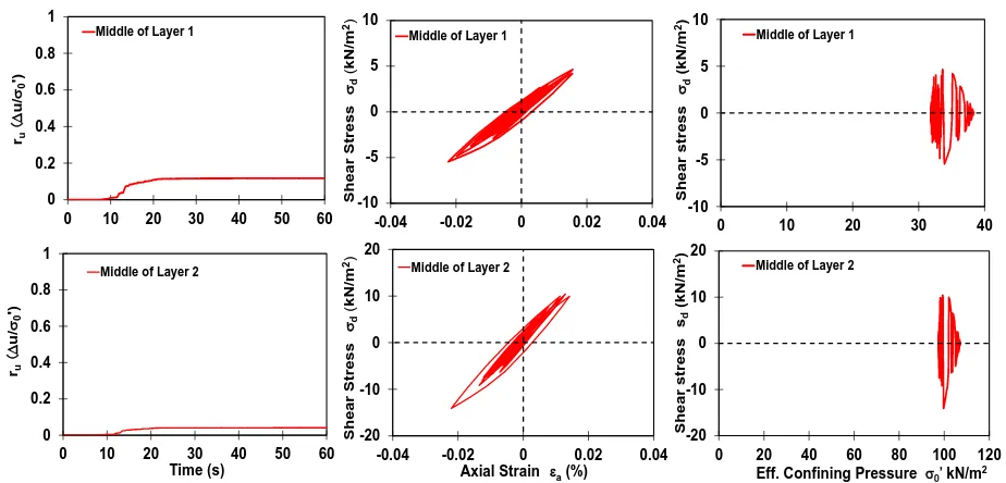
Figure 8 presents the soil behaviour at C-1. For the first sand layer, the excess pore water pressure ratio or ru

significantly builds up within 15 seconds and almost reaches 1.00, which indicates that liquefaction is possible. In addition, the cyclic loading resulted from the Tarlay Earthquake shaking results in the reduction of shear modulus, which is signed by the flattered hysteresis loop. This may be caused by a decrease in confining pressure due to the excess pore water pressure. Meanwhile, the low soil resistance is not sufficient enough to retain from the liquefaction during earthquake. For the second layer, the earthquake shaking also triggers the excess pore water pressure in a brief time. However, there is no liquefaction observed, since the maximum excess pore water pressure ratio is about 0.5. Shear modulus is also degraded in this layer. However, the reduction is not as much as the first sand layer. The effective confining pressure only decreases by 30 kPa. In general, the available soil resistance for the second layer is larger than the first sand layer; therefore, the earthquake shaking is not strong enough to generate liquefaction in the second layer. For the last layer, there is no indication of liquefaction, since the excess pore water pressure ratio is very small.

The interpretation of soil behaviour under the PGA of 0.070g at C-2 site is presented in Fig. 9. In general, the first two sand layers experience a reduction of effective confining pressure during the earthquake. However, the excess pore water pressure ratio generated by the propagated input motion is only 0.04 to 0.12. This indicates that the available soil resistance in C-2 is relatively sufficient to stand from the liquefaction resulting from the earthquake shaking. In addition, at the deeper depth, the excess pore water pressure is very small. Therefore, it can be concluded that there is no indication for liquefaction to occur on this site.

Figure 11 depicts the soil behaviour at C-4 during the Tarlay Earthquake. Similar to C-2 and C-3, the ground motion applied at C-4 is not large enough to generate excess pore water pressure ratio approaching 1.00. In addition, there is no indication of the significant reduction of effective stress. The hysteresis loop resulted during the wave propagation shows that there is no insignificant reduction of shear modulus. It indicates that the effective confining pressure is not significantly decreased due to the excess pore water pressure. The small amount of excess pore water pressure is also observed at the deeper layer, which has the large soil resistance. Therefore, there is no indication for C-4 site to undergo liquefaction during the Tarlay Earthquake.

Fig. 6. Generated input motion based on attenuation model analysis.

Fig. 7. Liquefaction Resistance Curve. -0.12

-0.08 -0.04 0 0.04 0.08 0.12

0 10 20 30 40 50 60

A

c

c

e

le

r

ati

on

(g)

Time (sec)

PGA = 0.0700g

C-2

-0.12 -0.08 -0.04 0 0.04 0.08 0.12

0 10 20 30 40 50 60

A

c

c

e

le

r

ati

on

(g)

Time (sec)

PGA = 0.038g

C-3

-0.12 -0.08 -0.04 0 0.04 0.08 0.12

0 10 20 30 40 50 60

A

c

c

e

le

ra

ti

o

n

(g

)

Time (sec)

PGA = 0.024g

C-4

0 0.1 0.2 0.3 0.4 0.5

1 10 100

Cyclic Str

ess Ratio

(



/2





)

N (cyclic)

1st Layer of C-1 2nd Layer C-1

1st Layer of C-2 2nd Layer of C-2

1st Layer of C-3 2nd Layer of C-3

3rd Layer of C-4 4th Layer of C-4

Mase et al.[24] (Osaka Sand) Tatsuoka and Silver [25] (Monterey Sand)

Gauchan [26] (Chiang Mai Sand) Yang and Sze [28] (Toyoura Sand)

Fig. 8. Soil behaviour of sand layers on C-1.

Fig. 9. Soil behaviour of sand layers on C-2.

0 0.2 0.4 0.6 0.8 1

0 10 20 30 40 50 60

ru ( D u/ 0 ') Time (sec)

Middle of Layer 1

-4 -2 0 2 4

-2 -1 0 1 2

She ar Str ess d ( kN /m 2)

Axial Strain a(%) Middle of Layer 1

-3 -2 -1 0 1 2 3

0 3 6 9 12 15

She ar st ress d (kN/ m 2)

Eff. Confining Pressure 0' kN/m2 Middle of Layer 1

0 0.2 0.4 0.6 0.8 1

0 10 20 30 40 50 60

ru ( D u/ 0 ') Time (sec)

Middle of Layer 2

-30 -20 -10 0 10 20 30

-0.1 -0.06 -0.02 0.02 0.06 0.1

She ar Str ess d (kN/ m 2)

Axial Strain a(%) Middle of Layer 2

-30 -20 -10 0 10 20 30

0 10 20 30 40 50 60 70 80

She ar st ress d (kN/ m 2)

Eff. Confining Pressure 0' kN/m2 Middle of Layer 2

0 0.2 0.4 0.6 0.8 1

0 10 20 30 40 50 60

ru ( D u/ 0 ') Time (s) Middle of Layer 1

-10 -5 0 5 10

-0.04 -0.02 0 0.02 0.04

Sh ea r Stress d ( kN /m 2)

Axial Strain _a(%) Middle of Layer 1

-10 -5 0 5 10

0 10 20 30 40

She ar st ress d (kN/ m 2)

Eff. Confining Pressure 0' kN/m2

Middle of Layer 1

0 0.2 0.4 0.6 0.8 1

0 10 20 30 40 50 60

ru ( D u/ 0 ') Time (s) Middle of Layer 2

-20 -10 0 10 20

-0.04 -0.02 0 0.02 0.04

She ar Str ess d ( kN /m 2)

Axial Strain a(%)

Middle of Layer 2

-20 -10 0 10 20

0 20 40 60 80 100 120

She ar st ress sd (kN/ m 2)

Eff. Confining Pressure 0' kN/m2

Fig. 10. Soil behaviour of sand layers on C-3.

Fig. 11. Soil behaviour of sand layers on C-4.

Generally, the first sand layer of C-1 is probable to undergo liquefaction during the Tarlay Earthquake. For the other sites, i.e., C-2 to C-4, the liquefaction is not possible. The low ground motions applied in C-2 to C-4 seems to be not significant to result in the energy for generating liquefaction. In addition, the large soil resistance is available at the deeper depth on each investigated site. Therefore, the bearing capacity of soil is sufficient enough to retain from the reduction of effective stress caused by excess pore water pressure. Based on the results, the liquefaction damage is estimated to happen only in the first sand layer of C-1. The result is in accordance with Soralump and Feugaugsorn [2], Ruangrassamee et al. [4], Mase et al. [29], and Mase

et al. [30] studies who mentioned that the liquefaction during the Tarlay Earthquake is only found on Mae

Sai (the border of Thailand Myanmar) or C-1 in this study.

0 0.2 0.4 0.6 0.8 1

0 10 20 30 40 50 60

ru ( D u/ 0 ') Time (s)

Middle of Layer 2

0 0.2 0.4 0.6 0.8 1

0 10 20 30 40 50 60

ru ( D u/ 0 ') Time (s)

Middle of Layer 3

-4 -2 0 2 4

-0.05 -0.025 0 0.025 0.05

Shear Str ess d ( kN/ m 2)

Axial Straina(%)

Middle of Layer 2

-6 -3 0 3 6

-0.02 -0.01 0 0.01 0.02

She ar Str ess d ( kN /m 2)

Axial Strain _a(%)

Middle of Layer 3

-4 -2 0 2 4

0 5 10 15 20 25 30

She ar st ress d (kN/ m 2)

Effective Confining Pressure 0' kN/m2 Middle of Layer 2

-6 -3 0 3 6

0 10 20 30 40 50 60 70

She ar st ress d (kN/ m 2)

Eff. Confining Pressure ₀' kN/m2 Middle of Layer 3

0 0.2 0.4 0.6 0.8 1

0 10 20 30 40 50 60

ru ( D u/ 0 ') Time (s) Middle of Layer 3

0 0.2 0.4 0.6 0.8 1

0 10 20 30 40 50 60

ru ( D u/ 0 ') Time (s) Middle of Layer 4

-3 -2 -1 0 1 2 3

-0.01 -0.005 0 0.005 0.01

She ar Str ess d ( kN /m 2)

Axial Strain a(%) Middle of Layer 3

-4 -2 0 2 4

-0.01 -0.005 0 0.005 0.01

She ar Str ess d ( kN /m 2)

Axial Strain a(%)

Middle of Layer 4

-3 -2 -1 0 1 2 3

0 5 10 15 20 25 30 35 40

Shear stress

d

(kN/

m

2)

Effective Confining Pressure 0' kN/m2 Middle of Layer 3

-4 -2 0 2 4

0 10 20 30 40 50 60 70

She ar st ress d (kN/ m 2)

Eff. Confining Pressure 0' kN/m2

6.

Concluding Remarks

This study discusses a seismic wave propagation analysis using the non-linear approach for the case study in the Northern Thailand, which underwent the 6.8 Tarlay Earthquake in March 2011. The NGA model analysis and one-dimensional site response analysis are conducted to observe the soil behaviour of liquefied layer during the Tarlay Earthquake. Some important conclusions are listed below:

1) The NGA analysis shows that the PGA values on some sites are less than 0.1g. According to Kramer [18]

and Day [19], the liquefaction potentially occurs under the earthquake with the minimum PGA of 0.1g

and magnitude of 5 Mw.

2) The NGA model analysis shows that C-2, C-3, and C-4 sites are not possible to undergo liquefaction

during the earthquake. The prediction of the liquefaction is furthermore confirmed by the result of the non-linear site response analysis, which shows that the applied ground motions are not capable of generating liquefaction.

3) C-1 could undergo liquefaction at a shallow depth i.e., the first 3 m depth, which is dominated by the

sandy soils with a relatively low soil resistance. The results are also consistent with the liquefaction evidences found in Mae Sai (C-1) district.

4) The results of this study are generally able to help reach an understanding of liquefaction potential. The

results are also addressed to the people living in Northern Thailand in order to escalate the awareness of the earthquake impacts, which can happen in the future.

Acknowledgement

The research was supported by the Thailand Research Fund Grant No. DBG-6180004 and the Ratchadapisek Sompoch Endowment Fund (2017), Chulalongkorn University (760003-CC). The work was performed under the Japan-ASEAN Science and Technology Innovation Platform (JASTIP-WP4). The authors would like to thank Dr. Suttisak Soralump for providing relevant data and useful suggestions throughout the research. The first author would be grateful for a Ph.D. scholarship from the AUN/SEED-Net (JICA).

References

[1] T. Ornthammarath, “A note of the strong ground motion recorded during the Mw 6.8 earthquake in

Myanmar on 24 March 2011,” Bull. Earthq Eng, vol. 11, no.1, pp 241-254, 2013. doi:10.1007/s10518-012-9385-4

[2] A. Ruangrassamee, T. Ornthammarat, and P. Lukkunaprasit, “Damage due to 24 March 2011 M6.8

Tarlay earthquake in Northern Thailand,” in Proc of 15th World Conference on Earthquake Engineering

(WCEE), Lisboa, Portugal, 24-28 September, 2012.

[3] Thai Meteorological Department (TMD), “Earthquake data of Thailand in 2011,” Thailand

Meteorological Department, Bangkok, Thailand, 2015.

[4] S. Soralump and J. Feungaugsorn, “Probabilistic analysis of liquefaction potential: the first eyewitness

case In Thailand,” in the 18th National Convention of Civil Engineering (NCCE), Chiang Mai, Thailand, May 8-10, 2013.

[5] Google Earth. (2017). Mae Sai-Mae Lao (Northern Thailand Region) [Online]. Available:

http://www.google.com [Accessed: 17 March 2017]

[6] W. Tanapalungkorn and S. Teachavorasinskun,“Liquefaction susceptibility due to earthquake in

Northern Parts of Thailand,” (in Thai) in the 20th _{National Convention of Civil Engineering (NCCE),}

Chonburi, Thailand, July 8-10, 2015.

[7] L. Z. Mase, S. Likitlersuang, S. Soralump, and T. Tobita, “Empirical study of liquefaction potential in

Chiang Rai Province in the North of Thailand,” in the 28th KKHTCNN Symposium on Civil Engineering, Bangkok, Thailand, 16-18 November, 2015.

[8] H. B. Seed and I. M. Idriss, “Simplified procedure for evaluating soil liquefaction potential,” Soil

Mechanics and Foundations Div, ASCE, vol. 97, no. SM9, pp. 1249–273, 1971.

[9] I. M. Idriss and R. W. Boulanger, “Semi-empirical procedures for evaluating liquefaction potential

[10] National Earthquake Hazards Reduction Program (NEHRP), “Recommended provisions for seismic regulation for new building and other structure, 1997 edition, Part 1-provisions, Part 2-commentary,” FEMA 302, Federal Emergency Management Agency, Washington, WA. 1998

[11] N. A. Abrahamson and W. J Silva, “Summary of the Abrahamson & Silva NGA ground-motion

relations,” Earthquake Spectra, vol. 24, no. S1, pp. 67–97, 2008.

[12] D. M. Boore and G. M. Atkinson, “Ground motion prediction equations for the average horizontal

component of PGA, PGV, and 5%-damped PSA at spectral periods between 0.01 and 10.0 s,”

Earthquake Spectra, vol. 24, no. S1. pp. 99–138, 2008.

[13] K. W. Campbell and Y. Bozorgnia, “NGA ground motion model for the geometric mean horizontal

component of PGA, PGV, PGD, and 5%-damped linear elastic response spectra for periods ranging from 0.01 to 10 s,” Earthquake Spectra, vol. 24, no. S1, pp 139–171, 2008.

[14] B. S. J. Chiou and R. R. Youngs, “An NGA model for the average horizontal component of peak ground

motion and response spectra,” Earthquake Spectra, vol. 24, no. S1, pp. 173–215. 2008.

[15] I. M. Idriss, “An NGA empirical model for estimating the horizontal spectral values generated by

shallow crustal earthquakes,” Earthquake Spectra, vol. 24, no. S1, pp. 217–242, 2008.

[16] T. Morita, S. Iai, L. Hanlong, K. Ichii, and Y. Sato, “Simplified parameter determination procedure for

computer program of evaluating damage to structures induced by liquefaction,” (in Japanese) Port and Harbour Research Institute, Tokyo, Japan, 1997.

[17] R. D. Miller, J. Xia, C. B. Park, and J. Ivanov, “Using MASW to map bedrock in Olathe, Kansas

(Exp.Abs),” J Soc. Explor. Geophys, vol. 1, pp. 433–436, 1999.

[18] S. L. Kramer, “Liquefaction,” in Geotechnical Earthquake Engineering. 1st ed. New Jersey: Prentice Hall,

1996.

[19] R. W. Day, “Liquefaction,” in Geotechnical Earthquake Engineering Handbook, 1st ed. New York:

McGraw-Hill, 2002

.

[20] S. Iai, Y. Matsunaga, and T. Kameoka, “Strain space plasticity model for cyclic mobility,” Soils and

Foundation, vol. 32, no. 2, pp. 1-15, 1992.

[21] K. Ishihara, F. Tatsuoka, and S. Yasuda, “Undrained deformation and liquefaction of sand under cyclic

stresses,” Soils and Foundations, vol. 15, no. 1, pp. 29–44, 1975.

[22] S. Iai, Y. Matsunaga, and T. Kameoka, “Analysis of undrained cyclic behaviour of sand under

anisotropic consolidation,” Soils and Foundations, vol. 32, no. 2, pp. 16-20, 1992.

[23] S. Sawada, O. Ozatsumi, and S. Iai, “Analysis of liquefaction induced residual deformation for two types

of quay walls: analysis by “FLIP”,” in the 12th _{World Conference in Earthquake Engineering (WCEE),}

Auckland, New Zealand, 30 January-4 February, 2000.

[24] F. Tatsuoka and M. L Silver, “Undrained stress-strain behavior of sand under irregular loading,” Soils

and Foundations, vol. 21, no.1, pp. 51-56, 1981.

[25] L. Z. Mase, T. Tobita, and S. Likitlersuang, “One-dimensional analysis of liquefaction potential: A case

study in Chiang Rai Province, Northern Thailand,” Earthquake Engineering Div, JSCE, vol. 73, no. 4, pp.I_135-I_147, 2017.

[26] J. Yang and H. Sze, “Cyclic behaviour and resistance of saturated sand under non-symmetrical loading

condition,” Geotechnique, vol. 61, no. 1, pp. 59-73, 2011.

[27] J. Gauchan, “Liquefaction tests on sand using a cyclic triaxial apparatus,” M.Eng. thesis, School of Eng

and Tech, AIT, Bangkok, Thailand, 1984.

[28] K. L. Lee and H. B. Seed, “Cyclic stress condition causing liquefaction of sand,” Geotechnical and

Geoenviromental Engineering, ASCE, vol. 93, no. SM1, pp. 47-70, 1967.

[29] L.Z. Mase, T. Tobita and S. Likitlersuang, “One-dimensional analysis of liquefaction potential: A case

study in Chiang Rai Province, Northern Thailand,” Journal of Japan Society of Civil Engineers, Ser. A1

(Structural Engineering & Earthquake Engineering (SE/EE)), Vol. 73, No. 4, pp. 135 – 147, 2017.

[30] L.Z. Mase, S. Likitlersuang, T. Tobita, S. Chaiprakaikeow and S. Soralump, “Local site investigation of

liquefied soils caused by earthquake in Northern Thailand,” Journal of Earthquake Engineering (Online