Some aspects of estimation of fractal dimension and stochastic simulation

(1)

I

n

Some Aspects of Estimation of

Fractal Dimension and

Stochastic Simulation

by

Grace W. S. Chan

A thesis submitted for the degree of Doctor of

Philosophy of the

Australian National University

(2)

I

Declaration

Chapter One of this thesis reviews work published by others in order to provide background and motivation for the work that follows. Unless otherwise stated in the text, the remaining chapters describe my own work, supervised by Professor P. G. Hall, Mr. D. S. Poskitt and Dr. A. T. A. Wood and published jointly with them.

(3)

ll

Acknowledgements

I wish to express my gratitude and thanks to the members of my supervision committee, Professor Peter G. Hall, Mr. Don S. Poskitt and Dr. Andrew T. A. Wood, for introducing me to the subjects studied in this thesis. Their support, encouragement and guidance throughout the course of this study were essential to this thesis. I also thank CSIRO Division of Mathematics and Statistics for providing the electrolytically zinc-plated data for this study.

I also wish to express my appreciation to the ANU, particularly the Depart-ment of Statistics in the Faculty of Economics and Commerce and the Statistical Science Program in the Centre for Mathematics and its Applications, for their financial support and facilities that ad made this study possible. I thank m em-bers and visitors in both departments for their support and assistance, which make my time at ANU the most enjoyable.

I am particularly indebted to my family in Hong Kong for their endless love and moral support. I am very grateful for their visit to Canberra and attending my wedding during the course of this study; and to numerous special friends, for their friendship and advice.

(4)

ill

Related Publications

The following papers have been submitted for publication from the work in this thesis:

Chan, G., Constantine, A. G. and Hall, P. G. (1994) Stochastic fractal models for multi-processed surfaces. Technometrics, submitted.

Chan, G., Hall, P. G. and Poskitt, D. S. (1994) Periodogram-based estimators of fractal properties. Annals of Statistics, under revision.

Chan, G. and Wood, A. T. A. (1994) An algorithm for simulating stationary gaussian random fields. Applied Statistics, Algorithm Section, submitted.

(5)

I

-lV

Abstract

In this thesis we discuss the use of Hausdorff dimension to characterize surface roughness. We also develop a new simulation method. In particular, we model surface line transects using Gaussian processes and provide a periodogram-based estimator of Hausdorff dimension from such data. In cases when the surface is the result of multi-processing we suggest simple stochastic models and modify the periodogram-based estimators to estimate Hausdorff dimensions for the penulti-mate and ultimate stages of the surface. Simulation study is often useful in this kind of study, and so we develop a simulation method based on circulant embe d-ding to generate multi-dimensional Gaussian processes. The thesis is divided into four chapters.

The first chapter provides background and motivation for our later work. In particular, we give a brief introduction to the different definitions of fractal di-mension, and we discuss in some detail the connection between Hausdorff dime n-sion and the roughness parameter, which we call fractal index, in the covariance function for Gaussian processes. Moreover, we review literature on simulation methods and explain why a new method is needed.

(6)

:

J

'

V

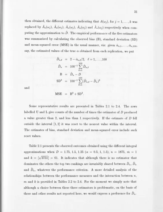
argue that the cosine part of the periodogram is more appropriate than the full periodogram for this application. The term semiperiodogram is used to describe the cosine component, and our estimator is based on simple linear regression of the logarithm of the semiperiodogram on the logarithm of frequency.

In some physical applications the fractal model describes the result of grinding or polishing a surface. This processing often involves several stages of varying :fineness, which might be likened to finishing a timber surface using different grades of sandpaper. Numerical analysis of surfaces that are produced in this way sometimes reveals traces of a penultimate processing step, involving a Haus-dorff dimension which differs from that in the final stage. An example of such data is the electrolytically zinc-plated surface. Simple stochastic models of this phenomenon are developed in Chapter 3. We also extend our theory for Haus-dorff dimension estimator in Chapter 2 to the estimation of both penultimate and ultimate Hausdorff dimensions for processed surfaces.

(7)

I

Vl

PROP

-ERTIES

1 Introduction . . . .

2 Methodology and Basic Properties .

2.1 Introduction and summary .

2.2 Methodology

2.3 Bias . .

2.4 Variance

2.5 Discussion

3 Numerical Results .

3.1 Sampling design and integral approximation

Vll

16

18

19

22

23

24

27

3.2 Simulation study . . . . . . . . . . . . 30

4 Proofs

4.1

4.2

4.3

Proofs of Theorems 2.1-2.3

Proof of Theorem 2.4

38

47

50

3 STOCHASTIC FRACTAL MODELS FOR MULTI-PROCESSED

SURFACES 52

(9)

-2

3

4

5

Stochastic Models .

2.1

2.2

2.3

Summary . . . .

Increasing roughness

Decreasing roughness . . . .

Methodology and Basic Properties .

3.1

3.2

3.3

Summary . .

Methodology

Basic properties

Numerical Results . . . . . . . . . . .

4.1 Simulated roughened process .

4.2 Simulated smoothed process

4.3 Zinc-plated surface

Proofs . . . .

5.1

5.2

5.3

5.4

Proof of Theorem 3.3 . . . .

Proofs of Theorems 3.4 and 3.5

Vlll 54 54 55 58 61 61 61 67 69

70

72 78 78 78 82 83

(10)

I

'

1

2

3

4

Introduction . . . .. . . . _.. _{. . . .} _{. . . . .} _.

The One-Dimensional Case . . . . .

The General N-Dimensional Case . . . . . . . .

Approximate Circulant Embedding

lX

86

88

91

97

5 The Simulation Procedure . . . . . . . . . . . . . . . . . . . . . . 98

5.1 The one-dimensional case . . . . . . . . . . . . . . . . . . 98

5.2 The N-dimensional case . . . . . . . . . . . . 99

6 Numerical Results . . . . . . . . . . . . . . . . . . . . . . . 102

6.1 Examples with CPU timings . . . . . . . . . . . . . . . . . 102

6.2 Comparison with Gibbs sampler . . . . . . . . . . . 107

7 Proofs . . . . . . . . . . . . . . . . . . . . . . . . . 112

7.1 Proof of Theorem 4.1 . . . . . . . . . . . . . . . . . . . 113

7.2 Proof of Theorem 4.2 . . . . . . . . . . . . . . . . . . . . . 114

7.3 Proof of Theorem 4.3 . . . . . . . . . . . . . . 115

(11)

X

List of Tables

2.1 Comparison among different approximations when n

=

1875, m

=

1, k

=

61 . . . . . . . . . . . . . . . . . . . . . . . . . 32

2.2 Comparison among different values of n and k when m

=

1 for

D

n

33

2.3 Comparison among different values of k when n

=

1875 and m

=

1

for

Dn

....

...

.

.. .

34

2.4 Comparison among different values of m and k for

Dn

with n

=

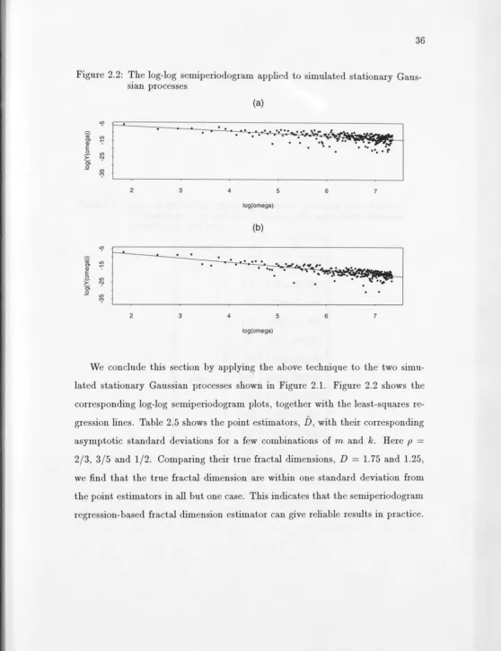
1875 34

2.5 D1942 for simulated stationary Gaussian processes when different

combinations of m and k are chosen (with asymptotic standard

deviations in bracket) . . . . . . . . .

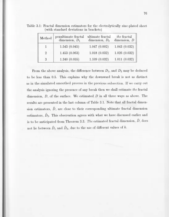
3.1 Fractal dimension estimators for the electrolytically zinc-plated

sheet ( with standard deviations in brackets) . . . . .

4.1 Average CPU timings in seconds with c

=

100 in all cases. (An 37

76

ast risk indicates that an approximate embedding was used.) . . . 106

4.2 Comparison betw en true and stimated correlations with

(12)

Xl

4.3 Comparison between true and estimated correlations with co

(13)

I

..

Xll

List of Figures

2.1 Simulated stationary Gaussian processes . . . . . . . . . . . . . . 17

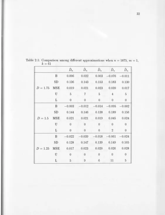
2.2 The log-log semiperiodogram applied to simulated stationary

Gaus-sian processes . . . . . . . . . . . . . . . . . . . . . . . . . . . . . 36

3.1 Zinc-plated surface and its log-log semiperiodogram plot 53

3.2 Increasing roughness processes . 57

3.3 Decreasing roughness processes 59

3.4 The log-log semiperiodogram and cumulative averaged log-log

semiperi-odogram plots of the simulated ultimate processes . . . . . . . . . 64

3.5 Two segments of length 500 of one of the zinc-plated line trace and

their estimated correlations 73

3.6 Two standardized sequ nces and their normal quantile-quantile plots 74

3. 7 Log-log mean semiperiodogram and the cumulative averaged

log-log mean semiperiodogram plots of the electrolytically zinc-plated

(14)

I

-Xlll

4.1 (1, 1) stationary Gaussian processes of length n

=

50000 with co-variance function ( 4.30) where c

= 100

and a

=

0.5, 1.0, 1.5, 1.9 respectively . . . . . . . . . . . . . . . . . . . . . . . 103

4.2 (2, 1) stationary Gaussian processes of length n

= (100 100) with

covariance function (4.31) where c = 100 and a= 1.0, 1.9 respec

t-ively .. . . .. . .

4.3 Comparison between the Circulant Embedding method and the 104

(15)

1

Chapter

1 FRACTAL DIMENSION AND STOCHASTIC

SIMULATION

1 Int

r

oduction

What are fractals? What is fractal dimension? Before we answer these questions,

let us go back to something we are all familiar with - point, line and disk. They have (topological) dimensions 0, 1, and 2 respectively. However, mathematically there exist many objects in between those mentioned which have non-integer dimensions. Mandelbrot (1975a, 1977) invented the term fractal to describe these objects. They can be a collection of points, lines, curves and even graphs. They can also be either deterministic or random and either self-similar or self-affine. Their dimensions depend on their complexity. The more complex they are the hjgher their dimensions.

(16)

I

•

2

volume 54 (1992).

There has also been considerable interest in modelling real phenomena using self-similar processes. One particularly popular application is to the problem of describing surfaces. For example, the surface of a fractured metal bar or of a highly magnified polished metal sheet, may be modelled in this way. Often the data obtained from surfaces are in the form of line transect samples, and so the self-similar process under study is a curve in the plane rather than a surface in three dimensional space. In this context, some recent developments in time series analysis are of interest, namely work that has focused attention on processes exhibiting long range dependence. Such processes are characterised by a power spectrum proportional to an inverse power law near the origin and have covariances that decay slowly; examples are fractional Brownian motion, due to Mandelbrot & Van Ness (1968), and fractional differences, introduced by Granger

&

Joyeux (1980), and Hosking (1981), both of which have been used to model

strongly dependent behaviour in economics, geophysics and hydrology. Various approaches to the estimation of parameters of interest in strongly dependent processes have been proposed, including the rescaled range and frequency domain methods. The former are discussed by Mandelbrot (1975b) and Mandelbrot &

Taqqu (1979) while Fox & Taqqu (1986), Geweke & Porter-Hudak (1983), Janacek (1982) and Kashyap & Eom (1988) consider the latter. Cox (1984) and Hampel (1987) provide general reviews of many of these ideas.

(17)

I

..

3

we develop a new simulation method, which is fast and "exact in principle", to simulate required realizations.

In Section 2 we give a brief introduction to Hausdorff measure and dimension. Section 3 discusses the relationship between the Hausdorff dimension and the covariance function of Gaussian or Gaussian-like processes. In Section 4 we give a literature review on simulation methods and explain why a new simulation method is needed. Finally, in Section 5 we provide a summary of topics studied in the remainder of this thesis.

2 Hausdorff Measure and Dimension

Hausdorff measure and dimension, also known as Hausdorff-Besicovitch dimen-sion, were first introduced in Hausdorff (1919). In this section we define Hausdorff measure and dimension and list some of their properties.

Let U denote a non-empty subset of ]RN. We define the diameter of U as

IUI

=

sup{lx -yl: x,y EU}.

If {Ui} is a countable (or finite) coll ction of sets of diameter at most 8, we say {Ui} is a 5-cover of F if

00

F C

LJ

Ui with O

<

IUil

'.S

8 for each i. i=l

For F a subset of ]RN, s a non-negative number and 8 > 0, we define

rl'/i(F)

=

inf {

~

IUil" : {Ui} is a 8-cover of

F}

(1.1)

(18)

I

ii

J

4

Now we define the s-dimensional Hausdorff measure of F,

1-i"(F)

=

lim 1-is(F).

0-+0 (1.2)

This limit exists for any subset F of !RN, though the limiting value can be zero or infinity. The quantity 1-i" is a measure and has the following properties:

(i)

'H"(0)

=

O;

(ii) 1-i"(E) ::; 1-i"(F) if E C F;

(iii) If {Fi} is countable sequence of sets then

1-i" (

lJ

Fi) ::;

f,

1-i"(Fi). •=l t=l

The equality holds if the Fi are disjoint Borel sets.

(iv) If F C !RN and A

>

0 then

A "1-i" ( F)

where AF = {Ax : x E F}.

(v) If F C !RN and

f:

F - !Rd is a mapping such that

l

f

(x)-

J(y)J ::;

cJx -

y

J°',

where x, y E F, c

>

0 and a

>

0, then for each s,

Equations (1.1) and (1.2) imply that for any given set F and 5

<

1, 'H7;(F)

and 1-i"(F) are non-increasing with s. There is a critical value of s at which

1-i"(F) "jumps" from infinity to zero. This critical value is called the Hausdorff dimension of F, and is written dimF:

That is

dimF

=

inf {s : 'H"(F)

= O}

sup{s: 1-i"(F)

= oo

}.

{

oo if s < dimF

1-i"(F)

=

(19)

I

•

(i) If F C !RN is open, then dimF

=

N.

(ii) If F is a continuously differentiable d-dimensional surface of ]RN then dimF

=

d.

(iii) If E

c

F then dimE S dimF.

(iv) If F1,

F2

,

.

..

is a (countable) sequence of sets then

dim(

_lJ

F

i

)

=

sup (dimFi )-•=l . 1:=;i<oo

(v) If Fis countable then dimF

=

0.

( vi) If F C !RN and

f

:

F ---+ ]Rd satisfies a Holder condition

l

f(

x) -

f

(y)I

S

clx

-yl

°'

x,y

E

F

for constants c > 0 and a> 0. Then dimf(F) S (1/a)dimF.

(vii) If

f :

F ---t ]Rd is a Lipschitz transformation, i.e.

l

f(

x)-

f(y)

I

~

clx-yl

x,

y

E

F

where c

>

0, then dimf(F) S dimF.

(viii) If

f

:

F ---+ ]Rd is a bi-Lipschitz transformation, i.e.

cilx

- YI

S

l

f(

x)

-

f(y)

I

S

c2lx -

YI

x, Y

E

F

where O

<

c1 S c2

<

oo, then dimf(F)

=

dimF.

5

(20)

The former estimated pointwise dimension via local exponent for time series. The latter estimated Hausdorff dimension via two types of approximate likelihood

(21)

6

There are many different notions of fractal dimension, some pertaining to sets

and some pertaining to distributions and time series. Examples include

(mod-ified) box-counting dimension, capacity dimension, compass dimension,

correla-tion dimension, covering dimension, divider dimension, information dimension,

Lyapunov dimension, mass dimension, Minkowski-Bouligand dimension, packing

dimension and pointwise dimension. See Billingsley (1986), Cutler (1990, 1991), Falconer (1985, 1990), Farmer et al. (1983), Mandelbrot (1977, 1982) and Taylor

(1986). In principle there can be a difference between the values suggested by

different notions of fractal dimension for a given object. However, in the context

of Gaussian or Gaussian-like processes, which is the case considered in this thesis,

all applicable notions give the same value. See Fischer (1993) for further details.

There exist many different ways to estimate fractal dimension in practice.

Cutler & Dawson (1989, 1990) discussed the nearest neighbour estimator of the

local Hausdorff dimension. Hunt (1990) and Sullivan & Hunt (1988) estimated

the capacity dimension by box-counting and quadrature methods respectively.

Broomhead & Jones 198 ) and Ogata & Katsura (1991) used maximum like li-1 ns-a

.-+ .;,.,

I; f-_ 1;. p 't.

hoodtpubuc et a. (1989a, 1989b) introduced the variation method for profiles

and surfaces. Virtually all methods for estimating fractal dimension are based on

so-called scaling laws, which involve seeking approximately linear relationships

between the logarithm of a certain estimable function and the logarithm of its

argument. There are many possible choices for the function. We refer the reader

to Berry & Hannay (1978), Brown et al. (1993), Burrough (1981), Carr & Benzer

(1991), Carter et al. (1988), Coster & Chermant (1983), Delfiner & Delhomme

(1975), Ling(1987: 1989, 1990), Majumdar & Bhushan (1991), Mandelbrot et al.

(1984), Sayles & Thomas (1978), Serra (1968), Taylor & Taylor (1991), Thomas & Thomas (1988), among others. More references are listed at the end of the

next section.

In this thesis we shall focus on Hausdorff dimension of the graph of a Gaussian

(22)

7

now on. In the next section, we shall discuss how to estimate fractal dimension

for graphs which can be modelled using stationary Gaussian processes.

3 Fractal Dimension and Gaussian Processes

Chapter 8 of Adler (1981) provides a detailed discussion of fractal dimension for

a range of Gaussian processes. We recall some of the relevant results here.

Define an

(N

,

d)

Gaussian field to be a ]Rd-valued Gaussian random field on

N· JR ' i.e.

We assume that X has mean 0, continuous covariance function and homogeneous

increments, i.e. the d incremental variance functions

o-f(s

,

t)

=

E{

I

X

i

(s)-X

i

(t)l2}

,

for i= l, ...

,

d

,

are functions of s -

t

only. Next we definite the index-{3, (N, d) Gaussian field.

DEFINITION 1.1 (Adler (1981), Definition 8.3.1} Let

X(t)

be an (N, d) Gaus

-sian field, such that each Xi has zero-mean, stationary increments, and a continu -ous covariance function. For each i

=

1, ... , d set

o;(t)

=

E{

I

X

i

(s

+

t)-X

i

(s)12}

.

Then if for each i

=

l, ... , d there exists a

/3i

such that

/3

i

= sup{/3:

o

i

(t)

=

o

(iltll

.B

)

,

lltll

l

O} = inf{/3:

l

ltl

l.B

=

o

{o

i

(t)}

,

ll

t

ll

l

O},

(1.3)

and O

<

f3i :=:; 1, we call X an index-{3 Gaussian field for {3

= (

/31, ...

,/3

d)-Adler has pointed out that an important special case of (1.3) occurs when

(23)

8

for each i, and O

<

Ci

<

oo. He also proved the following theorem and corollary

which enable .us to establish a very direct and simple relationship between fractal dimension dim or D and index (3. Before we state the theorem we need to introduce notation and regularity conditions.

Write

E

(t)

for the covariance matrix of the vector

X(t)

-

X(O)

,

so that

the diagonal elements of

E(t

)

are the incremental variance functions

o-f

(

t)

=

E{IXi(t) - Xi(O)l2}. We assume that there exists E

>

0, such that for all t E

J

;

=

[-1, l]N,

det E

(t)

d

>

E.

IL

=1

a-f

(t)

(1.4)

Write the graph and image of X as

GrX

=

{(t,X(t)):

t

E Io} C !RN+d

and

lmX

{X

(t) :

t

E

1

0} C !Rd,

where 10

= [O

,

l]N C ]RN.

THEOREM 1.1 {Adler

{

1981

),

Theorem

8.4.1)

Let X be an

(N

,

d) Gaussian

field on IO

=

[O, 1

]N

of index f3

,

with coordinates so arranged that the

f3

satisfy

If {1.4) holds and the <Ti(t) are bounded away from zero on

1 ;

=

[-1, l]N fort

bounded away from the origin, then, with probability one,

dim(ImX)

dim(GrX)

.

{d

N

+

I:,

f=

1 (/3d

-

/3i)

}

mm ,

/3d

,

min { N

+

I:,

f=;:/3d

-

{Ji),

N

+

t(l

-

/3i

)}

{

dim(ImX) if dim(lmX) < d,

(24)

9

COROLLARY 1.2 (Adler {1981), Corollary on P.204) Let X be as in the

theorem, and suppose that each coordinate field has the same incremental variance

function, with the same index j3. Then, with probability one,

dim(ImX) min

(d

,

;)

,

dim(GrX) min {; , N

+

d(l -

/3)

}

.

In this thesis we are interested only in ( N, 1) stationary Gaussian processes

of the form

with covariance function

,(

t

)

=

,(O) -

cll

t

ll

0

+

o(ll

t

ll

0

) , as

11t11

- t 0,

where N

2'.

1, c

>

0 and O

<

a

:S

2. Hence X has incremental variance function

given by

a2(s

,

t)

E{IX(s) - X(t)l2}

2 {,(O) -

,(lit -

s

1/

)}

2

cll

tll

0

+

0

(11

t

11°).

According to Definition 1.1, Xis an index-~, (N, 1) Gaussian process. And

Corollary 1.2 implies that dim( GrX) has fractal dimension,

1 D

=

N

+

1- -a.

2 (1.5)

Hence, w can calculate or estimate fractal dimension via the roughness parameter

(25)

10

and so D

=

N

+

l - ½2

=

N, as expected. In practice most curves and surfaces of interest have fractal index less than 2. In this case, the fractal dimension is fractional, and lies strictly between N and N

+

l. The relationship (1.5) between fractal dimension and fractal index persists for a variety of non-Gaussian processes, but not for all such processes. For example, if X

=

I

Z

I

"

,

where Z is a Gaussian process with zero mean and v

>

-

½

,

then (1.5) holds if and only if v

2'.

½-

See Hall & Roy (1994) for further details.

The idea of estimating fractal dimension via modelling observed data as Gaus -sian process has been discussed in Constantine & Hall (1994), Feuerverger et al. (1994), Hall (1994) and Hall & Wood (1993). They have employed the box -counting, level crossing counting and variogram methods to estimate the fractal index and hence fractal dimension. In this thesis, we suggest a technique for estimating fractal index based on the periodogram.

4 Literature Review on Simulation Methods

There is a sizeable geostatistics literature on simulating N-dimensional stationary

Gaussian processes. Our main sources are the helpful reviews given by Ripl y

(1987) (section 4.5) and Cressie (1991) (section 3.6), the ref rences given in those

two books, and papers in recent volumes of the journal Mathematical Geology.

In order to put our approach into context and explain why it fills a gap in this

literature, we briefly mention arlier proposals without giving any details of the

methods concerned.

(26)

11 is moderately large. Let us consider N-dimensional stationary Gaussian process

on a rectangular grid

{

j

(j[l]

j[N])T

.

}

t = - = - · · · - : 0

<

J[f..]

<

n[f..]

-1 1

<

f..

<

N C [0 l)N C rr:r,N

n

n[l] '

'

n[

N]

-

'

-

'

~

'

where j[l] and n[l] are integers with n[l] ~ 1 fixed for 1 -::;

e-::;

N. If ii.=

TT

~

₁n[f] is sufficiently large ( e.g.

n

~ 1200), Cholesky factorization of the relevant covar i-ance matrix is not feasible, a consequence of the fact that storage requirements of the Cholesky approach are O(n2₎_. _For_e_xampl_e,_Ch_oles_ky_{factorization}_o_f_a

matrix of order 50,000 x 50,000 is beyond the capacity of any computer. In con -trast, our approach can comfortably deal with

n

=

50,000 in many cases, even

on a relatively modest computer.

A second possibility, which is widely used for simulating isotropic

Gaus-sian processes on !RN, is the "turning bands" method. See Bras & Rodriguez-Iturbe (1985), Brooker (1985), Cressie (1991), Christakos (1987), Dimitr

akopou-los (1990), Journel

&

Huijbregts (1978), Mantoglue (1987), Mantoglue

&

Wilson (1982), Matheron (1973) and Ripley (1987). However, as noted by all these

au-thors, the turning bands method for simulating isotropic Gaussian processes is

approximate because it depends on application of a central limit theorem. So, the turning bands approach is not "exact in principle".

A variety of one-dimensional and multi-dimensional spectral methods have been proposed. However, with one exception, which is discussed below, all the proposals based on spectral methods that we have seen require one of three types

of approximation: either the invocation of a central limit theorem, or the in-exact treatment of "edge effects", or approximation of the covariance function by a function which has compact support. Whether such approximations are of consequence from a practical point of view is highly context-dependent, but it is clear that if any of the three approximations mentioned above is made, then the resulting procedure will not b exact in principle. For further details of

(27)

12

et al. (1981), Mejia & Rodriguez-Iturbe (1974), Miller & Borgman (1985), Rice (1954), Shinozuka (1971) and Shinozuka & Jan (1972).

Another possibility is to use spatial nearest-neighbour or autoregressive mod-els; see Martin (1979, 1990, 1991), Sen (1989, 1990, 1991), Sharp & Aroian (1985,

1989) and Smith & Freeze (1979a, 1979b). Assuming that we wish to view the covariance function as prescribed, as is the case here, this kind of approach has the following significant drawback: the resulting autoregressive structure will not be sparse except in very special circumstances. There is also a question mark over whether it is feasible to implement this kind of approach exactly in principle when the number of grid points is at least moderately large (e.g.

n

~ 1200).

Davis (1987) has suggested an approximate approach based on the idea of approximating the square root of the covariance matrix by a matrix polynomial. Black & Freyberg (1990) proposed the one-dimensional moving average approach, which is exact in principle if the relevant covariance matrix is a type of band matrix but not otherwise.

Finally, we mention an iterative simulation method - the Gibbs sampler. See Gelman & Rubin (1992) and Tanner (1993). Although the domain of application for the Gibbs sampler is not the same as our method, there are situations which both methods can be applied, e.g. the Ornstein- Uhlenbeck process. It requires a similar amount of storage to our method but it is not "exact in principle".

(28)

er-In practice, roughness measuring instruments record thousands of measurements across a very sho,rt distance. For example, the zinc-plated surface data presented in Chapter 3 were recorded at 3885 equally-spaced points over a line transect

1

mm long. We can rescale and relocate the process into the interval

[-

1,

1]

without loss of generality. Information about the length of the process and the surface type may be obtained via the scale parameter c in the covariance function.

Our asymptotic theory is based on the number of sampled points increasing over the interval. We show that the cosine part of the periodogram, which we call

the semiperiodogram, has certain advantages over the full periodogram in the context of estimating fractal index. It can be estimated via the slope of the approximately linear relationship between the logarithm of semiperiodogram and the logarithm of frequency. Of course, there are other besides the p riodogram

and semiperiodogram for estimating fractal dimension in the frequency domain

(29)

13

ror, assessment of the accuracy of the procedure is likely to become far more complicated.

5 Summary of Thesis

Often data obtained from surfaces are in the form of line transect samples, e.g. the electrolytically zinc-plated data. Thus in Chapters 2 and 3 we restrict our attention to index-}, (1, 1) stationary Gaussian processes, or simply referred to as stationary Gaussian processes. Now we have

where O

<

a ~ 2.

1

D

=

2- - a

2 ' (1.6)

In Chapter 2 we suggest a technique for estimating fractal index a, and hence (using formula (1.6)) fractal dimension D of the sample paths of a stationary Gaussian process, based on the periodogram. We assume that the data are in the form of a trace of the process in the continuum. The trace need not be a long one.

our asymptotic theory is based on a trace over a fixed interval, which we

<:;ce_ take without loss enerality to be [-1, 1]. We show that the cosine part of the

L _ hAi-0

I

periodogram, which we call setni-periodogragi.,.-h s certain advantages over the

?.1.,y::

I

full periodogram in the context

~~

fractal index. It can be estimated

I

via the slope of t e-- proximately linear relationships between_ the logarithm of se · oa.ogram and the logarithm of frequency.

---==---,

(30)

14

the surface's life. In the first of these examples the penultimate roughness is greater than the ultimate roughness, although this inequality is reversed in the

latter two cases. Statistical calculations of surface roughness sometimes reveal evidence of both ultimate and penultimate processing operations. In Chapter 3 we suggest simple stochastic models for repeated polishing steps, and show that

the data which derive from these models do exhibit the features observed in practice. In particular, they produce a "broken stick" linear regression of the

logarithm of periodogram, or semiperiodogram, on logarithm of frequency. The break is upward in the case of increasing roughness, and downward for decreasing roughness.

We should stress that in Chapters 2 and 3 all our theory is conducted under the semi-parametric model

1

(t)

=

1

(0) -

c/t/

0

+

o(/t/

0 ) as

t

-+

0 ,

rather than a fully parametric model such as

,(t)

=

exp(-c/t/0

) . It is easy to show that an estimator based on the latter assumption is inconsistent if the model is misspecified.

Often a simulation study is useful for examining the numerical performance of new estimation methods such as those introduced in Chapters 2 and 3. It

is desirable to have realizations which are "exact in principle" in the simulation study. In Chapter 4 we introduce the Circulant Embedding Simulation Method. It is a method for simulating (N, 1) stationary Gaussian processes with prescribed covariance function on a fine rectangular grid in

[O

,

l)N C ]RN. It is assumed that the proc ss is stationary with respect to translations of ]RN, but the method does not require the process to be isotropi·c. As with some other approaches to this simulation problem, our procedure uses discrete Fourier methods. A notable

(31)

II

15

to apply the procedure are (i) the covariance function is summable on ]RN and

(ii) a certain spectral density on the N-dimensional torus, which is determined

by the covariance function on ]RN, is strictly positive. The procedure can cope

with more than 50, 000 grid points in many cases, even on a relatively modest

computer. An approximate procedure is also proposed, to cover cases in which it

(32)

II

16

Chapter

2 PERIODOGRAM-BASED ESTIMATORS OF

FRACTAL PROPERTIES

1 Introduction

The fractal properties of the sample paths of a stationary Gaussian process may be described very simply in terms of the behaviour of its covariance function at the origin. For example, if the stationary Gaussian process X has covariance given by

,(s - t)

=

co

v{X(s)

,X(t)},

and if

,(t)

=

_{1(0) -}

citl

0

+

o(ltl

0

)

(2.1)

as

t

-

0, where 0

<

a ~ 2 and c

> 0, th

en a is called the fractal index of X. The fractal or Hausdorff dimension of X, equivalent also ( on the present occasion) to other dimension definitions, is given by

1 D

=

2- -a.

2

(2.2)

(33)

(\J

~

·1.0

(\J

·1.0

Figure 2.1: Simulated stationary Gaussian processes

(a)

·0.5 0.0 0.5

time

(b)

·0.5 0.0 0.5

time

17

1.0

In practice we are mainly interested in processes with fractal dimension greater

than 1 (i.e. 0

<

a

<

2). When we study roughness of a surface, e.g. an

electrolytically zinc-plated surface, we let X denote the surface height of the

transect sample curve above an arbitrary fixed level. We observe X at points on

a grid and assume that X may be modelled as a stationary Gaussian process.

For the purpose of analysis based on the periodogram or semiperiodogram, we

rescale the location of the transect to [-1, 1] and refer to it as time. Figure 2.1

illustrates two simulated stationary Gaussian processes with covariance function

of the form

,(t)

=

exp(--cltl0

) ,

wher

(

c,a

)

=

(1, 0.5) and (1, 1.5). Hence fractal dimensions ar qual to 1.75

and 1.25 respectively. Note that the roughness of the surfac transect decreases

with its fractal dimension. To make it easier to compar with the zinc-plated

(34)

I '

18

these processes are chosen to be the same as the real data, 3885.

In this chapter, we suggest a technique for estimating fractal index, and hence (using formula (2.2)) fractal dimension of the sample paths of a stationary

Gaus-sian process, based on the periodogram. We assume that the data are in the form of a trace of the process in the continuum. The trace need not be a long one.

Indeed, our asymptotic theory is based on a trace over a fixed interval, which we take without loss of generality to be [-1, 1]. Issues of aliasing, i.e. of discretizing a continuous trace on a grid, are discussed both theoretically and numerically. We show that the cosine part of the periodogram has certain advantages over the full periodogram in the context of estimating a.

We should stress that all our theory is conducted under the semi-parametric

model (2.1), rather than a fully parametric model such as ,(t)

=

exp(-citl°'). It is easy to show that an estimator based on the latter assumption is inconsistent if the model is misspecified.

In Section 2 we introduce our estimator and derive its basic properties, includ-ing bias, variance and asymptotic distribution. In Section 3 we discuss numerical issues and summarize the result of a simulation study. Proofs of theorems in Section 2 are deferred to Section 4.

2 Methodology and Basic Properties

2.1 Introduction and summa~y

Our estimator of fractal index is based on a version of the periodogram for a continuous trace of a stochastic process X. The definition of the continuum p riodog1:am, I, is similar to that of the periodogram computed from discrete

(35)

-...

19

observations of X , and is given in Subsection 2.2. It is composed of both cosine and sine parts. We define the semiperiodogram, J, to be the cosine part of the periodogram. Subsection 2.2 provides asymptotic formulae for expected values of both the cosine and sine components of I, assuming a regularity condition similar to {2.1). Those results imply that when a

>

1 the value of a cannot be

estimated directly from the periodogram, but that the semiperiodogram can be

employed successfully whenever O

<

a

<

2. Therefore we focus attention on the semiperiodogram, and define an estimator 6: based on regression of log J on the logarithm of frequency.

Bias and variance of 6: are discussed in Subsections 2.3 and 2.4 respectively.

The size of bias depends critically on behaviour of the "o(ltl°')" term in {2.1),

and so that expansion must be elaborated upon if we are to describe bias. Sub -section 2.5 discusses the overall performance of 6:, explaining concisely how the accuracy of 6: is affected simultaneously by both deterministic errors and stochas -tic fluctuations. We present a central limit theorem for the estimator, and address the issue of recording the data on a fine grid rather than in the continuum. This

matter of "aliasing", as it is often called, can influence the accuracy of our theo -retical description of the properties of 6:. We state an explicit condition on grid width that is sufficient to ensure that aliasing does not affect the central limit theorem for 6:.

Proofs of the theorems in Subsections 2.2 to 2.5 are given in Section 4.

2.2 Methodology

Let X d note a stationary Gaussian process observed on interval [- 1, 1], and define

A(w)

[

1

X(t)

cos

(wt) dt

,

B(w)

[ 1

1

(36)

..

I

20

I(w)

=

A(w)2

+

_B(w)2

, J(w)

=

A(w)2.

We call I the periodogram and J the semiperiodogram. Note that I(w)

=

I(- w),

J ( w)

=

J ( - w). If w is an integer multiple of 21r then, regardless of the mean of

X, E{A(w)}

=

E{B(w)}

=

0. Henceforth we suppose that w is a positive integer

multiple of 21r.

The theorem below states that if O

<

a:

<

2 then E{ J(w)} ,...., const . w-(0+1₎

as

w

.,

oo, and that the same is true of

E{J (

w)}

provided

O

<

a:

'.S

1. These properties form the basis of our approach to estimating

a:.

To state the theorem

we must introduce regularity conditions, which we do next.

Given ~

>

0,

let A(O denote the class of functions h on

(0

,

2)

such that,

sup

f

2

lh(t

+

u) - h(t)I dt

=

O(5e)

lul~5 }0

as 5 .,

0.

(We extend h from

(0,

2)

to (-oo, oo) by periodicity.) Note that, if 0

'.S

T/

<

1, the function h(t)

=

CTI is in A(l -

rt)

-

Given a real-valued function g,

let g', g", . .. or equivalently 9(1), 9(2), . .. denote its successive derivatives. Define

91 by

,(t)

=

_{1 (0)}- ct0

+

91(t), t

>

0,

(2.3)

for constants c

>

0 and 0

<

a:

<

2 (as in (2.1)). We assume that for some E

>

0,

g~ E A(o:

+

c) (if

a:

< 1)

or g~ E A(o:

+

c - 1) (if 1

'.S

a:

< 2)

. (2.4)

For 5

>

0, put

K{,i"}(- 5)

=

f

00

r 5

{ sin }(t)dt,

co,

lo

cos

respectiv ly. H r , th sine and cosine functions should be taken respectively.

We note that

Ksin(-5) f(l - 5) COS (

?f/)

0 < b

<

2,

(37)

21

THEOREM 2.1 Assume condition

{2.4).

Then, as w ---t oo through integer multiples of 21r,

E{A(w)2} - w-1

fo\2

-

t) ,'(t) sin(wt) dt

l

2caw-(2cw-2 c.r+l)Ksin(a -1)

2ca (a - l)w-(c.r+l)Kcos(a - 2)

if O <a< 1 if a= 1

if 1 <a< 2 2 cr(a

+

1) sin (1r

2a) 0 <a< 2,

-w-1

fo

2

(2 - t) ,'(t) sin(wt) dt

+

2w-2

fo

2

,'(t) cos(wt) dt

+

2w-2 {,(0) - ,(2)}

2caw-(c.r+l)Ksin(a - 1) if 0<a<l

2 { C

+

_{1 (0) -}

_{1 (2)}}w-2 if a= l

2 {,(O) - ,(2)} w-2 _i_f

1 <a< 2.

(2.5)

(2.6)

In view of the theorem, logE{J(w)} ,...,

-(a+

l)logw for 0 <a:::; 1, but

log E{ I (

w)}

,...,

-2 log

w for

1 < a

<

2. Thus, in the case a

>

1 we cannot expect

to be able to estimate a in terms of the slope of the regression of log I ( w) on

logw. On the other hand, logE{J(w)},...,

-(a+

l)logw for 0 <a< 2, so that

regression of log J(w) on log w is practicable for estimating a in this wider range.

Therefore we focus attention on the semiperiodogram.

Let u(w)2 = E{A(w)2}, Z(w) = A(w)/u(w), Y(w) = log A(w)2, e(w) =

log Z(w)2

- E{log Z(w)2}, C₁ = E{log Z(w)2}. Since Z(w) has the Standard

Normal distribution for each w then C1 does not depend on w. This is corr

e-sponding to an exact scaling law. In this notation,

Y(w) = log a(w)2

+

C1

+

e(w).

Formula (2.5) may be writt n as u(w)2

,...., C2w-(c.r+1l, where C2

>

0. This obser

-vation prompts the approximate r gressiou model,

Y(w) '.::::'. C3 -

(a+ l)logw

+

e(w),

where C3 = C1

+

log C2 . That in tum suggests to estimate a based on the least

(38)

"'"

---

1

-22

multiples of 21r. Put Xj

=

log Wj,

x

=

k-1

I:

Xj, Yi

=

Y(wj),

The systematic and random errors of this estimator are described by bias and variance, respectively. We treat them separately. To simplify exposition we take

Wj

=

21rmj, l ::; j ::; k, where the integer m

=

m(k) 2:'. 1 may depend on k and could diverge to positive infinity as k --+ oo.

2.3 Bias

The size of bias is determined by the

"

o(IW·)"

term in

(2.

1 )

,

corresponding to 91 in (2.3). In order to be explicit about bias it is necessary to enter into more detail about properties of

9

1 . With this in mind we shall refine

(2.4)

to the new condition (2.8), below.

Define 92 by

1 (t)

=

1(0) - ct0 - dta+{3

+

d't 2

+

92(t), t

>

0, (2.7)

for constants c

>

0,

d

>

0,

d'

E Ill, 0

<

a

<

2, 0

<

/3

<

1, /3

i-

2 - a. We assume that for some E

>

0,

Put

Me

=

-9~ E A ( a +

/3

+

E) (if

a+/3

<

1) or

g;

E A(a

+

/3

+

E - 1) (if 1::; a+

/3

<

2)

or g;'EA(a+/3+E-2) (if

2<a+f3<3)

.

Ksin(( - 1), if 0

<

l

<

1

1 if

l

=

l

< ₍₍_- _l)K_cos((_{- 2)} if 1

<

(

<

2

0 if

l

=

2

-(l -

1)(( - 2)Ksin(( - 3) if 2

<

l

<

3

r(flsin

(

~l

)

0

<

(

<

3,

(2.8)

(39)

-23

THEOREM 2.2 Assume condition (2.8). Then, as m(k) and k ---+ 00

1

2.

4 Variance

If the variables Yj

=

Y ( Wj) were stochastically independent then variance would

be given by

var(&)

-

{

t(

•;

-

x)

'f

~ar(Y,)

Of course, the Yjs are not independent, but we claim that nevertheless, this variance formula is asymptotically correct, as evidenced by the following theorem.

THEOREM 2.3 Assume condition (2.4), and that ,"'(t)

=

O(t°'-3

) as t

l

0.

Then, as k ---+ oo,

(2.10)

We should comment on the fact that, in Theorem 2.3, the asymptotic variance of

a

does not depend on m, although that quantity does appear in our asymptotic formula for bias; see Theorem 2.2. The fact that m does not enter the first-order asymptotics for var( a) is a consequence of our definition of the design points,

Xj

=

log(27rmj); note that m vanishes from the centred design points Xj -

x.

For other choices of design, in particular for Wj /271' equal to the integer part of

(40)

...

Ill

24

2 .

5 Discussion

The conditions of both Theorems 2.2 and 2.3 hold if we assume that for some

E

>

0, the function 92 appearing in (2.7) satisfies

(2.11)

as

t

1

0. In the event that the conditions of both theorems hold, we may deduce

from those results that as k ---t oo,

where the random variable Wk has zero mean and variance s2

=

var{log N(O, 1)2 }.

Thus,

a

-

o: in probability ask - oo. If m(k) is chosen so large that k1

-2f3m-213

-0 as k ---t oo (for example, if m

2-

1 in the case {3

>

1/2), then k112(a - o:) has

asymptotically zero mean and variance s2• Quite generally, k112(a. -Ea.) has an

asymptotic Normal distribution, as our next result shows.

THEOREM 2.4 Assume condition (2.4)) _{and that 1}<4

)(t)

=

O(t''-

4) as t

1

0. Then k1₁2₍_{a -} _Ea.) _is_{asymptotically}_No_rmally_distributed_with_zero_{mean and} variance s2

.

Condition (2.11) is sufficient for the assumptions of Theorem 2.4.

In practice, the integrals defining A(w1 ), . . . , A(wk), and hence

a,

would

usu-ally be approximated by series computed from points of a grid. So, we should

state a result which points out that if the grid points are sufficiently closely spaced

theu our asymptotic results continue to hold. In the discussion above we noted

that k1₁2₍_{a -} _o:₎_has_a_noudegen_rate_di_stribution_,_and_so_it_suffices_{to describe}_a series-based approximation to

a:

which is accurate to terms of smaller order than

k-1

(41)

....

-

1

--25

To this end, define

n-1

An(w)

=

n-1

I::

X(i/n) cos(iw/n),

i=-n

our approximation to A(w) based on a (2n)-point grid. Let &n denote the

corresponding approximation to

a,

computed with An(wj) replacing A(wj) for 1 ~ j ~ k. Our next theorem shows that if n

= n(k) in

creases sufficiently rapidly

then a - an= o(k-112), so that (for example) an - Ea satisfies the same central limit theorem as a - Ea.

THEOREM 2.5 Assume condition

{2.

4 ),

and th_{at I} is decreasing on an inter -val ( 0,

t:

)

J

or

t:

>

0 sufficiently small. Suppose n

=

n( k) - t oo so fast that

(2.12)

as k -t oo. Then k1l2(a - an)-+ 0 with probability one.

We suspect that condition (2.12) is substantially more severe than is necessary

m practice, and our simulation study indicates this too. However, in strictly

rigorous theoretical terms we have not been able to improve on it. The effect of

discretizing the time variable, commonly called aliasing, will be taken up in more

detail in the next section. It should be stressed that the problem is aggravated

by the requirement that we examine the spectral density for large values of its

argument, w; for small values the effects of aliasing are much less. However, there

seems no way of avoiding this difficulty.

The cosine and sine parts of th p riodogram are not, individually, shift

in-variant - that is, the random processes

A(w, A)

=

1-~

X(t) cos{w(t

+

A)} dt and B(w, A)

=

[

1

1 X(t) sin{w(t

+

A)} dt

ar non-d g nerate functions of A as w 11 as w. (The full periodogram, {A(w, A)2

+

B(w, A)2

}, and their squar d xp ctations, E{A(w, A)2} and E{B(w, A)2}, do not

(42)

-..

I

26

depend on A.) This property may be used to enhance the performance of the e sti-mator&, as follows. Let a(A) denote the same function of

A(wi

,

A), ... ,

A(wk

,

A) as & was of

A(wi),

...

,

A(wk);

let v 2:'.: 1 be an integer; let Ai, ... , Av be arbitrary real numbers; and put

V

ao v-i

La(

Aj). j=i

The distribution of a(A) does not depend on A, and so

E(&o)

=

E(&), var(&o) ~ var(&).

It follows that in mean-squared error terms, &0 performs at least as well as &,

and possibly a little better.

To appreciate the extent of any improvement offered by &0 we must evaluate

its variance. To this end, note that

A(w

,

Ai)/a-(w) and

A(w

,

A2

)

/

a-(w)

have a

bivariate Normal distribution with zero means, unit variances, and correlation

coefficient equal to

uniformly in Ai and A2, as w ---+ oo. Let

g(p)

denote the covariance of (log

N;

,

logNn if (Ni,N2 ) are bivariate Normal N(O,O; 1,1,p). Then

g(p)

depends only on

IPI

,

and is strictly positive unless

p

=

0, in which case

g(p)

=

0. Hence the asymptotic variance of &0 equals

which for appropriate choice of v(---+ oo) and Ai, ... , Av is asymptotic to k-iTJS2

where 0

<

T/

<

1 and s2

=

var{log N(O, 1)2}.

(43)

However, in practice roughness mcasunng instruments only produce e

qually-spaced data. In this subsection, we will discuss the effect of different sampling

designs on our present problem based on simulation and conclude that we can

im-prove the approximation based on uniform sampling by assigning unequal weights.

We consider estimating A( w) using 2n

+

1 observations of the process X

at the points ti,n, i

=

-n, ... , n, over the interval [-1, 1], and employing an

(44)

27

of statistical efficiency, in terms of choice of v and the A's. The issue of aliasing has

been of much greater concern. However, the matter of statistical inconsistency,

in connection with practical estimation of fractal dimension via the periodogram

when a

>

1, has considerable practical interest.

3 Numerical Results

3.1 Sampling design

and integral

approximation

Recall from Subsection 2.5 that our initial approximation of semiperiodogram

A( w) is defined by

n-1

An(w)

n-1

L

X(i/n)

cos(iw/n). i=-n

This, of course, amounts to using a uniform sample design of 2n points on the

interval [-1, 1). It is known, however, that for the problem of approximating a

weighted integral of a stochastic process over a finite interval, uniform sampling

is not necessarily optimal. See Benhenni & Cambanis (1992) and the references

-

~

contained therein. More generally, therefore, we may consid @stinratmg A( w)

<::ec (r~+- using 2n

+

1 observations of the pTOeess

X

at the points ti,n, i

=

-n, ... , n, ove

1

cl

e~e .

~

-th ·n-te:rva:t""[-1, 1], and employing an approximation of the form _ _ J

n

A

n(w)

=

L

WiX(ti,n) cos(wti,n) i=-n

where th sample design { ti,n} and weights { wi} are chosen so as to minimise the

asymptotic mean-squared error

E{A(w)

-

A

n(w)

}2

;

see Benhenni and Cambanis

op. cit. This choice depends on covariance structure of the process. In the

simu-lations reported in Subsection 3.2 the underlying covariance function is assumed,

for convenience, to be of the fully parametric form

,(t)

=

exp(-cltl0

(45)

28

where c

>

0 and O

<

a

<

2. We shall therefore examine this case in a little more detail.

From the two differential equations given in (2.14) below it is straightforward

to verify that the regularity conditions required by Benhenni and Cambanis for

the determination of the optimal sample design are only applicable if we know

that a

=

l. There we find that {

ti

,

n

}

is obtained by solving

n +i 2n '

where the constant "-w is such that

[ 1

1

"-wl cos(wt)l2/3dt 1.

i

=

-n, ... ,n,

We have evaluated {

ti

,

n

}

for vanous combinations of w and n. We found

that only for small values of w does

lti

,

n

-

i/nl equal or exceed the length of the

uniform sampling interval; for moderate and large values the difference between

the optimal and uniform sampling points is less than n-1 _by_{an orde}_r_o_f_magnitude

at worst. Although the above results relate to the particular case a

=

1 it is clear

that the close proximity of

{t

i

,

n

}

and {i/n} for increasing w is brought about

by the increasingly rapid oscillations in

I

cos(wt)/2

/3 over [-1, 1], and it appears

reasonable to conjecture that the behaviour of the cosine function would similarly

dominate such calculations for other values of a, and the more general covariance functions as defined in (2.1). This suggests that in general very little may be

lost by using a uniform sample design. Indeed, in practice the true value of a is

unknown and we envisage estimating it using a range of frequency values. Thus,

the estimation process will be more convenient and versatile if the same set of

sampling points can be employed in all circumstances, as appears to be the case.

Once the sample design is known, determination of the weighting sequence

(46)

...

I

Ill ....

obtain

8,(t)

at

a

2 , (

t)

8t

2

- sgn(t) caitl°'-1 exp(-cltl°')

ca{caitl2°'-2 - (a - l)ltl°'-2}exp(-cltl°').

29

(2.14)

Since all a's of interest are less than two, these formulae confirm (Benhenni and

Cambanis, 1992, p.166) that the process has no quadratic mean derivative. Given that the optimal sampling design is closely approximated by the uniform sequence

{

i/n

}

,

particularly when w

=

21rf is large, then following the arguments presented immediately above we see that the optimal weighting is likely to differ little from the trapezoidal rule. Hence, in the simulation experiments that follow we shall

consider the performance of the quasi-optimal integral approximation

An(w)

=

n-

1 [ {(X(-1)

+

X(l)} /2 +_

I:

X(

i/n) cos(iw/n)

]

.

i=-n+l

With regard to the latter, it is perhaps of interest to observe that

An(w)

may be viewed as a conventional approximation based on tapered data. It is known that in the frequency domain analysis of time series, tapering can produce high resolution estimates with enhanced performance; see Dahlhaus (1988). As a basis

for comparison we shall therefore also investigate the alternative approximation

n-1

A. n

(w)

=

n-

1

L

X(i

/n) cos(i

w

/n

)h(i

/n),

i=-n

where h( ·) is the split cosine taper with cosine bell applied to 20% of the data.

Some aspects of estimation of fractal dimension and stochastic simulation

n