Determining hydraulic resistance in gravel-bed rivers from the dynamics of their water surfaces

Hydraulic resistance in gravel-bed rivers from the dynamics of their water surfaces 1839 Earth Surface Processes and Landforms

Earth Surf. Process. Landforms31, 1839–1848 (2006) Published online 23 October 2006 in Wiley InterScience (www.interscience.wiley.com) DOI: 10.1002/esp.1447

Letter to ESEX

Determining hydraulic resistance in gravel-bed rivers

from the dynamics of their water surfaces

James R. Cooper,

_{* Simon J. Tait}

_{and Kirill V. Horoshenkov}

Department of Geography, University of Hull, UK

2

Pennine Water Group, Department of Civil and Structural Engineering, University of Sheffield, UK

3

Pennine Water Group, School of Engineering, Design and Technology, University of Bradford, UK

Abstract

Traditionally, approaches to account for the effect of the boundary roughness of a gravel-bed river have used a grain-size index of the gravel-bed surface as a surrogate for hydraulic resistance. The use of a single grain-size does not take into account the spatial heterogeneity in the bed surface and how this heterogeneity imparts resistance on the flow, nor the way in which this relationship changes with variables such as flow stage. A new technique to re-motely quantify hydraulic resistance is proposed. It is based on measuring the dynamics of a river’s water surface and relating this to the actual hydraulic resistance created by a rough sediment boundary. The water surface dynamics are measured using a new acoustic tech-nique, grazing angle sound propagation (GRASP). This proposed method to measure hy-draulic resistance is based on a greater degree of physical reasoning, and this is discussed in the letter. By measuring acoustically the temporal dynamics of turbulent water surfaces over a water-worked gravel bed in a laboratory flume, a dependency is demonstrated between the temporal variation in the reflected acoustic pressure and measured hydraulic resistance. It is shown that the standard deviation in acoustic pressure decreases with increasing hydraulic resistance. This is shown to apply for a range of relative submergences and bed slopes that are typical of gravel-bed rivers. This remote sensing technique is both rapid and inexpensive, and has the potential to be applied to natural river channels and to other environmental turbulent flows, such as overland flows. A whole new class of low-cost, remote and non-intrusive instruments could be developed as a result and used in a wide range of hydraulic and hydrological applications. Copyright © 2006 John Wiley & Sons, Ltd.

Keywords: boundary roughness; hydraulic resistance; water surface; grazing angle sound propagation

*Correspondence to: J. R. Cooper, Department of Geography, University of Hull, Cottingham Road, Hull HU6 7RX, UK. E-mail: J.R.Cooper@hull.ac.uk

Introduction

A key problem in fluvial geomorphology has been the evaluation of the resistance imposed by different bed morphologies on the flow (Rouse and Ince, 1963). The determination of this flow resistance is a fundamental requirement for the prediction of flow depth, and thus the calculation of channel flood capacity and bed shear stress to estimate sediment entrainment and transport. Yet the ways in which this resistance is determined still remain crude. The magnitude of the resistance is known to be a function of the geometry of the bed surface. This geometry can only be fully characterized by considering the grain-size distribution, grain shape, grain orientation, bed arrangement, and concentration and geometry of features on the bed surface (Robert, 1990). Generally, in rivers, boundary roughness has been determined by accounting for the effects of all these features with a single coefficient ks, the equivalent sand roughness height,

such that for uniform, steady flow the mean velocity at a given cross-section U is estimated by (Keulegan, 1938)

U  (= gdS)

[

]

1840 J. R. Cooper et al.

where g is the acceleration due to gravity, d is the water depth and S is the channel slope. Traditionally, a particle diameter at a certain percentile of the grain-size distribution of the bed material has been used to define ks. In general,

this has been set equal to the order of 3·5D84 or 6·8D50 (see, e.g., Hey, 1979; Bray, 1982). This approach assumes that

the effect of the bed on the flow is spatially constant and has the same effect at all sites and at all flows, but in reality river bed surfaces are highly irregular and their effects are known to be greater at low flows than at high flows (Griffiths, 1989). As such, the hydraulic roughness characteristics of a river bed are poorly described and are poorly approximated by the use of a single grain-size index, for which the underlying physical basis is unclear. It is clear that alternative approaches to determining hydraulic resistance, which adopt a greater degree of physical reasoning, are required.

Several studies of flow turbulence have shown that the generation and evolution of vortically based large-scale flow structures create quasi-cyclic but persistent flow patterns over water-worked gravel beds (Kirkbride and Ferguson, 1995; Ferguson et al., 1996; Dinehart, 1999; Buffin-Bélanger et al., 2000; Shvidchenko and Pender, 2001; Roy et al., 2004). Once these features are formed, they migrate downstream, deform and amalgamate and produce circular regions of local upwelling on the water surface. Jackson (1976) was the first to describe a scenario in which a vortical flow structure interacts with the water surface, creating secondary vortices. Some studies have suggested that boil generation is the result of flow separation behind dunes. But, other studies have found that surface upwellings occur without the presence of significant bedforms (Kumar et al., 1998), and others have argued that there may be several different generation mechanisms for such water surface features (Kostaschuck and Church, 1993; Babakaiff and Hickin, 1996). Observations and measurements of vertical distributions of turbulent flow properties have indicated that large-scale flow structures dominate the transfer of fluid momentum and hence frictional losses between the bed and the fluid (Robert et al., 1996; Buffin-Bélanger et al., 2000). It appears reasonable, therefore, that an examination of the temporal dynamics of a water surface, and the expression of the large-scale flow structures beneath, may provide potential information about the resistance exerted by a water-worked sediment bed on the flow. This type of observation would be able to take into account the spatial roughness characteristics of the bed surface through the physical effect this has on the flow, something which is not described by the use of a grain-size index. Such an approach demonstrates a stronger degree of physical reasoning and, to the best of our knowledge, has not been carried out before.

It has been long realized that forward- or back-scattering strength and statistics of a transmitted signal can be linked to the spatial spectrum of a dynamically rough interface. In this context, sonar and radar methods have been previously developed for the characterization of the scattering strength of the fluid–air interface (Jackson et al., 1992; Dahl, 1999). These have been primarily used to study long-range underwater sound propagation and echo-sounding in open seas. Empirical spectra have been proposed (Kitaigorodskii, 1983; Durden and Vesecky, 1985) and used to relate wind speed to the spectral density of the sea surface roughness. This has been achieved successfully for the characterization of the dynamic ocean interface by relating the empirical spectra to the acoustic/electromagnetic scattering cross-section.

This paper attempts to develop an existing technique within acoustic engineering to remotely determine the hydrau-lic resistance imposed by water-worked gravel beds. The temporal dynamics of water surfaces over these beds are measured acoustically, for a range of flows simulated in a laboratory flume for which the hydraulic resistance has been quantified. The data presented shows that a relationship exists between hydraulic resistance and water surface beha-viour. The potential application of this method for remote physical measurement of this resistance is also discussed.

Methodology

Grazing angle sound propagation

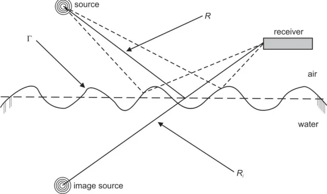
Recent advances in the study of the acoustics of rough surfaces have revealed that grazing angle sound propagation (here termed GRASP) can be used to determine remotely the geometrical and statistical characteristics of rough solid surfaces (Attenborough and Taherzadeh, 1995; Chambers and Sabatier, 2002) and fluid surfaces (Dahl, 1999). These studies have shown that GRASP has the potential to measure the typical scales of topographical variation in water surfaces for turbulent flows over rough sediment beds. This acoustic approach is based on the assumption that the sur-face roughness causes a certain perturbation to the acoustic wave R emitted by a point source, and that the reflections by the rough boundary Γ are received at a point receiver (Figure 1). The total sound pressure field at the receiver is p=g0+pβ, where

g e

R e

R

ikR ikR

i

i

0

4 4

= − −

− −

Figure 1. Schematic representation of the acoustic detection of dynamic roughness, whereby the surface roughness (in this case the water surface) Γ causes a perturbation in an acoustic wave R emitted by a point source, and reflections from the boundary are received at a point receiver.

is the Green’s function for sound propagation over a plane rigid boundary and

p ik e H sr s

k s k s k

ds

i z zs k s

β _πβ

β

( )

( ) ( )

=

−

(

)

−∞ ∞

+ −

4

2 2

01

2 2 2 2

is the perturbation term due to the surface roughness. In these expressions r is the horizontal distance between the source and receiver, k is the acoustic wavenumber, z and zs are the receiver and source heights, respectively, H0

(1)_(x)

is the Hankel function of the first kind of zero order of some quantity x and parameter β is the acoustic surface admittance. In the case of a perfectly smooth, rigid boundary the value of the admittance is β= 0 and the sound pressure is p ≡g0. It was shown by Attenborough and Taherzadeh (1995) that in the case of an acoustically rigid

boundary composed of stationary hemispheres of radius a (analogous to water surface upwellings) the acoustic admittance is purely imaginary and given by

β = − π  − π π 

  +

 

 

ik Na a

l

a l

2 3 2 3

3

2 3

3

3 1 4 1 4 (4)

where i = −1, N is the average density of hemispheres per unit area and l ≈ N is the mean spacing between the hemispheres. Equations (2)–(4) suggest that the acoustic pressure at the position of the receiver should depend on the instantaneous radius of the hemispheres and their spatial distribution. Applying the Thomasson (1980) approximation for integrals to Expression (3), we find that for grazing angles of sound propagation the acoustic pressure perturbation is pβ ~ βeikr/r, which incorporates the effect of the surface roughness. We note that this effect is averaged over the

intersection of the Fresnel ellipsoid and the reflecting boundary (Hothersall and Harriott, 1995). Here, the Fresnel ellipsoid can be defined as an ellipsoid with the minor axis of radius λ/3 and the foci being at the image source point and the acoustic receiver, where λ is the acoustic wavelength.

1842 J. R. Cooper et al.

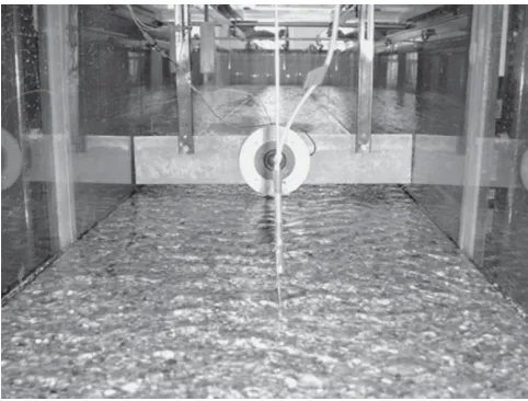
Figure 2. The experimental arrangement of the acoustic equipment, showing the microphone mounted on a thin rod from the flume rails in the foreground and the circular tweeter mounted on a horizontal traverse in the background. As a guide for scale, the separation between the glass walls of the flume is 0·5 m.

which were produced periodically at 100 ms intervals. A total of 40 sweeps were deployed for each water surface investigated. The signal was reflected by the water surface and the glass-sided walls of the flume. These signals were recorded by a 1/4″ microphone and de-convolved to determine the acoustic impulse response of these features. An Adrienne time window of 0 –1·4 ms was employed to control the multiple reflections from the glass walls so that the reflections from the water surface were optimized (Figure 3). A distance of 0·5 m was used between the microphone and the tweeter. This separation was found to allow the full development of the interference pattern between the outgoing acoustic wave and the acoustic wave reflected by the water surface. This in turn controlled the reflections received from the flume walls. The tweeter emitted a spherical wave so the water surface was acoustically detected over a streamwise distance of 0·5 m. The width of the detected area of which the reflections from the water surface were of importance was approximately equal to λ/3. Given that the tweeter was operated at a minimum frequency of 1 kHz, this resulted in a maximum width of 0·1 m. This experimental set-up produced a signal-to-noise ratio of greater than 20 dB in the frequency range of 2–30 kHz. The acoustic impulse response from the water surface for each of the 40 sweeps was determined by separating the acoustic pressure response received at the microphone from the radiated sinusoidal sweep stimulus. The standard deviation at time t of the 40 responses σp(t) was considered to be an

appropriate measure of the temporal variation in the elevation of the water surface and was given by

σ

p

j j

t

p t t

( )

( ) ( ) =

−

(

)

=

∑

1 40

40 (5)

where pj(t) is the acoustic pressure response for response j at t, and ∏(t) is the acoustic pressure response averaged

over 40 responses at t.

Experimental set-up

Figure 3. The acoustic pressure response p over time t showing the reflections of one acoustic signal from the water surface and the glass-sided flume walls. Also depicted is the form of the Adrienne time window applied to the acoustic pressure response to control the reflections from the flume walls.

Recently, Barison et al. (2003) discovered that the spatial distribution of time-averaged streamwise velocity over sediment beds in the near-bed region was significantly different over flat, scraped beds than over a water-worked bed. Initially when the bed was flat, the distributions were highly positively skewed, with a low proportion of smaller velocities. As the bed surface became more water-worked the distributions became flatter, wider and less skewed. This indicated that the way in which the beds are formed in the laboratory might have an important effect on the flow field. A different approach to bed production was therefore adopted here. A widely graded river sediment was fed into the flume during conditions in which the bedload transport capacity of the flow, as estimated by Meyer-Peter and Müller (1948), was half of the imposed sediment feed rate. This resulted in the progressive formation of a sloping water-worked gravel bed in the base of the flume (Figure 4(a)). The bed was formed through the movement and rearrange-ment of the individual grains by the flow, allowing the flow to sort the grains over the flume length. The sedirearrange-ment was fed into the flow with the use of a conveyor belt in order to maintain a steady feed rate. Feeding was halted once a steady bed slope was formed. The sediment mixture had a unimodal and lognormal grain-size distribution encom-passing medium sized gravels to fine sands, typical of gravel-bed rivers, with D50 of 4·97 mm and D84 of 7·00 mm

(Figure 4(b)).

A total of 15 hydraulic conditions were investigated (Table I). A range of flow depths was produced so that the ratio of d to D84 varied from 2·8 to 12·8, which is believed to be the typical range found in gravel-bed rivers (Robert, 2003).

The Reynolds numbers for all flows were high enough to ensure that all flows were fully turbulent. During the testing programme, the slope of the flume was less than that used during the formation of the bed, so that the deposit grains were stationary during all experimental runs. In each run the flume was set at a known channel slope and uniform, steady flow conditions were achieved, after which the water depth was measured and the mean flow velocity was calculated from the ratio of flow discharge to the cross-sectional area of the flow. This data enabled the hydraulic resistance ks for each flow condition to be calculated using an equation originally developed by Colebrook (1938) for

1844 J. R. Cooper et al.

U gRS k

R R gRS

s

( ) log

( )

= −

⋅ +

⋅ 



  32

14 8

1225 32

10

υ ₍₆₎

where R is the hydraulic radius, defined as the ratio of cross-sectional area of the channel to the wetted perimeter, and

υ is the kinematic viscosity. The temporal dynamics of the water surface was then measured using GRASP at a distance of 10 m from the flume inlet.

Table I. A summary of the investigated hydraulic conditions, where S is the channel slope, d is the water depth, D84 is the size of

the intermediate axis of the bed grains for which 84 per cent of the bed material is finer, U is the average flow velocity (calculated from the ratio of flow discharge to the cross-sectional area of the flow), and Re is the flow Reynolds number (calculated from

Ud/υ, where υ is the kinematic viscosity). It was ensured that a water temperature of approximately 23 °C was maintained so that the kinematic viscosity of the water was constant throughout all the experiments

Run S (-) d (mm) d/D84 ¨(m/s) Re (-) ks (mm)

1 0.00285 19.4 2.8 0.16 2 328 15.0

2 0.00285 30.6 4.4 0.25 5 773 10.4

3 0.00285 38.9 5.6 0.29 8 727 9.9

4 0.00285 49.2 7.0 0.34 12 925 9.6

5 0.00285 63.7 9.1 0.44 21 108 6.7

6 0.00285 89.7 12.8 0.58 39 669 3.9

7 0.00375 43.2 6.2 0.36 11 811 10.2

8 0.00375 49.4 7.1 0.40 14 928 9.5

9 0.00375 61.0 8.7 0.50 23 281 5.8

10 0.00465 29.5 4.2 0.29 6 477 13.1

11 0.00465 37.9 5.4 0.36 10 491 10.6

12 0.00555 32.8 4.7 0.35 8 763 11.6

13 0.00555 39.7 5.7 0.44 13 149 8.3

14 0.00645 32.7 4.7 0.37 9 298 12.2

15 0.00735 29.1 4.2 0.37 8 188 11.9

Results

Visual records were made of the water surfaces for several hydraulic conditions in order to examine whether the dynamics of the water surfaces changed with hydraulic resistance. Two images of water surfaces taken over the measurement area are provided as a visual guide to the range of the water surface behaviour observed (Figure 5). It can be seen that the water surface with a relatively high level of hydraulic resistance and a low water depth (Figure 5(a)) is characterized by many small upwellings, all of which are elongated laterally. In contrast, the surface with a low level of resistance and deeper water (Figure 5(b)) is much rougher in appearance and dominated by a smaller number of much larger upwellings, resembling a train of standing waves, as found in critical flow (Tinkler, 1997). Surrounded by these upwellings is a much flatter water surface.

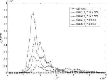
An examination of the change in σp(t) with ks provides a quantitative measure of the relationship between the

temporal dynamics of the water surface and hydraulic resistance (Figure 6). The results presented in Figure 6 were obtained by averaging the standard deviation in the acoustic impulse response within the time window shown in Figure 3. For clarity, only runs 1, 2, 3 and 6 have been included in Figure 6 along with the data from a still water surface as a basis for comparison. This shows that the standard deviation generally decreases for flows with higher ks

values. This effect is particularly pronounced for the peak values in the time period of 0·135– 0·156 ms. This time interval corresponds to the time of the arrival of the first acoustic reflections from the water surface. Outside this time period the effect of the roughness of the water surface on the acoustic impulse response is limited and the acoustic signal is contaminated with reflections from the walls of the flume (see Figure 3).

It is this time interval of 0·135– 0·156 ms that appears to be of most interest in determining whether the acoustic reflections from the water surface can determine hydraulic resistance. By examining the standard deviation in the acoustic pressure response averaged over this time interval <σp

2_{> and how this varies with k}

s, the potential of this

application can be discovered (Figure 7). It is clear that there is a dependence between <σp2> and ks. The temporal

variation in the acoustic pressure reduces with increasing ks values.

Discussion and Potential Applications

1846 J. R. Cooper et al.

Figure 6. The change in the standard deviation in the acoustic impulse response σp(t) with time t. Four hydraulic conditions are shown in order to show how the acoustic response changes with hydraulic resistance, and these are compared with a still water surface.

unlike through the use of a single grain-size index, in which the choice of grain-size involves no consideration of the variations in water depth or bedform geometries. This means that rapid measurement of hydraulic resistance could be achieved, which would allow the assessment of temporal changes in resistance during floods. This newly developed technique could also be used for a given river at different locations along its downstream course. Also, it does not require the time-consuming task of measuring the grain-size distribution of a river bed, which without careful sam-pling design can poorly represent the actual grain size-distribution and cause uncertainties in the estimates of bound-ary roughness.

The acoustic technique presented here determines hydraulic resistance by considering the interaction between the bed surface and the internal flow structure, and then examining the manner in which the internal flow structure is reflected in the dynamics of the water surface. As such, this technique has a strong element of physical reasoning, and its use in different river environments is not likely to be restricted by assumptions and simplifications that are inherent in the application of the grain-size index method. It therefore has the potential to be more widely applied to rivers with different morphologies and for the study of other turbulent flows, such as overland and in-pipe flows. The physical basis of GRASP means that it can provide estimations of boundary roughness that are responsive to changes in water depth. This technique is non-intrusive, inexpensive and rapid and is able to predict hydraulic resistance at times when this data is needed quickly, such as in flood forecasting. It will open up significant possibilities for river managers; model calibration could be significantly improved and on-line real-time monitoring become a realistic option.

Figure 7. The standard deviation in acoustic impulse response averaged over the time interval 0·135 ≤ t ≤0·156 ms <σp

2_>

against hydraulic resistance ks. This time interval corresponds with the time of the arrival of the first acoustic reflections from the water surface within each acoustic response. All fifteen experimental runs outlined in Table 1 are displayed.

Equation (4) suggests that the transition from a small laboratory to a large-scale in situ environment may require a proportional decrease in the frequency of the emitted sound in order to be able to remotely sense larger-scale water surface roughness observed in natural rivers and open channels.

The work reported in this letter aims to promote further studies into the dynamics of turbulent water surfaces, a currently neglected area of study. Although this letter has examined its potential for determining hydraulic resistance, it is clear that the water surface has the potential to provide additional information on the main structural aspects of the flow, and may provide insights into the behaviour of coherent flow structures that may not be easily detectable in velocity data. The data presented in this letter should encourage the development of a whole new class of instrument: remote, non-intrusive, low cost and deployable in a wide range of fluvial environments.

Acknowledgements

This work was supported by a platform grant awarded by the UK Engineering and Physical Sciences Research Council to the Pennine Water Group of the Universities of Sheffield and Bradford (GR/R47967/01). The work was completed whilst J.R.C. was in receipt of a University of Sheffield Project Studentship. This letter benefited from equal contributions from the three authors, and the suggestions of two anonymous reviewers.

References

Attenborough K, Taherzadeh S. 1995. Propagation from a point-source over a rough finite impedance boundary. Journal of the Acoustical Society of America98: 1717– 1722.

1848 J. R. Cooper et al.

Barison S, Chegini A, Marion A, Tait SJ. 2003. Modifications in near bed flow over sediment beds and the implications for grain entrain-ment. Proceedings of XXX IAHR Congress2: 509– 516.

Bray DI. 1982. Flow resistance in gravel-bed rivers. In Gravel-Bed Rivers, Hey RD, Bathurst JC, Thorne CR (eds). Wiley: Chichester; 109– 133.

Buffin-Bélanger T, Roy AG, Kirkbride AD. 2000. On large-scale flow structures in a gravel-bed river. Geomorphology32: 417– 435. Chambers JP, Sabatier JM. 2002. Recent advances in utilizing acoustics to study surface roughness in agricultural surfaces. Applied

Acoustics63: 795– 812.

Colebrook CF. 1938. Turbulent flow in pipes, with particular reference to the transition between smooth and rough pipe laws. Journal of the Institute of Civil Engineers11: 133– 156.

Dahl PH. 1999. On bistatic sea surface scattering: field measurements and modeling. Journal of the Acoustical Society of America105: 2155– 2169.

Dinehart RL. 1999. Correlative velocity fluctuations over a gravel river bed. Water Resources Research35: 569– 582.

Durden SL, Vesecky JF. 1985. A physical cross-section model for a wind-driven sea with swell. IEEE Journal of Ocean Engineering10: 445– 451.

Ferguson RI, Kirkbride AD, Roy AG. 1996. Markov analysis of velocity fluctuations in gravel-bed rivers. In Coherent Flow Structures in Open Channels, Ashworth PJ, Bennett SJ, Best JL, McLelland SJ (eds). Wiley: Chichester; 165– 183.

Griffiths GA. 1989. Form resistance in gravel channels with mobile beds. Journal of Hydraulic Engineering, ASCE115: 340– 355. Hey RD. 1979. Flow resistance in gravel-bed rivers. Journal of the Hydraulics Division, ASCE105: 365– 379.

Hothersall DC, Harriott JNB. 1995. Approximate models for sound propagation above multi-impedance plane boundaries. Journal of the Acoustical Society of America97: 918– 926.

Jackson FC, Walton WT, Hines DE, Walter BA, Peng CY. 1992. Sea-surface mean square slope from K(U)-band backscatter data. Journal of Geophysical Research—Oceans97: 11 411-11 427.

Jackson RG. 1976. Sedimentological and fluid-dynamic implications of turbulent bursting phenomenon in geophysical flows. Journal of Fluid Mechanics77: 531– 560.

Keulegan GH. 1938. Laws of turbulent flow in open channels. Journal of Research of the National Bureau of Standards21: 707– 741. Kirkbride AD, Ferguson R. 1995. Turbulent flow structure in a gravel-bed river: Markov chain analysis of the fluctuating velocity profile.

Earth Surface Processes and Landforms20: 721– 733.

Kitaigorodskii SA. 1983. On the theory of the equilibrium range in the spectrum of wind-generated gravity-waves. Journal of Physical Oceanography13: 816 – 827.

Kostaschuk RA, Church MA. 1993. Macroturbulence generated by dunes—Fraser-River, Canada. Sedimentary Geology85: 25– 37. Kumar S, Gupta R, Banerjee S. 1998. An experimental investigation of the characteristics of free-surface turbulence in channel flow. Physics

of Fluids10: 437– 456.

Meyer-Peter E, Müller R. 1948. Formulas for bed-load transport. Proceedings of Second Congress of IAHR, Stockholm. Robert A. 1990. Boundary roughness in coarse-grained channels. Progress in Physical Geography14: 42– 70. Robert A. 2003. River Processes: an Introduction to Fluvial Dynamics. Arnold: London.

Robert A, Roy AG, DeSerres B. 1996. Turbulence at a roughness transition in a depth limited flow over a gravel bed. Geomorphology16: 175– 187.

Rouse H, Ince S. 1963. History of Hydraulics. Dover: New York.

Roy AG, Buffin-Bélanger T, Lamarre H, Kirkbride AD. 2004. Size, shape and dynamics of large-scale turbulent flow structures in a gravel-bed river. Journal of Fluid Mechanics500: 1– 27.