Article
Remotely-Controlled Low-Cost Digital Telescope
Gaël Robin
1,a, Anant K. Shukla
2, and Romuald Jolivot
1,b,*1 BU-CROCCS, School of Engineering, Bangkok University, Bangkok, Thailand 2 BURL, School of Engineering, Bangkok University, Bangkok, Thailand
E-mail: a[email protected], b[email protected] (Corresponding author)
Abstract. This paper presents a low-cost web controlled digital telescope which can benefit
educational institutions. The system is composed of two webcams to acquire data. One is used as a wide field of view for localization purpose and the second one is used as a narrow field of view using a 40 cm focal length lens and an achromatic doublet to visualize celestial objects. The telescope orientation is performed remotely using two motors through Internet with an in-house developed software running on a Raspberry Pi 3 device. Message Queue Telemetry Transport (MQTT) based server is used to provide a full wireless communication between the user and the telescope for orientation control, data visualization and acquisition. The telescope structure is built using a 3D-printer. An image processing algorithm is presented to calibrate mounting camera misalignment. The overlapping calibration is performed to localize the telescope image onto the large field-of-view image. It is based on Fourier domain cross-correlation technique.
Keywords: Camera calibration, digital refractor telescope, image processing, Internet of
Things, MQTT application, Raspberry Pi application.
ENGINEERING JOURNAL Volume 23 Issue 3
Received 8 October 2018 Accepted 3 April 2019 Published 31 May 2019
1.
Introduction
Optical telescopes have always been a main source of interest for astronomers, amateurs and professional, thanks to their relative ease of assembly in both transmission and reflection schemes [1]. Astrophotography has significantly been improved with the development of digital image acquisition techniques in multiple spectral bands such as visible, radio, x-ray and gamma radiation ranges [2, 3]. For the visible domain, several technologies offer a large range of image acquisition systems ranging from USB webcams to higher end sensors. The images can be further enhanced using image processing techniques [4, 5]. Controlled mechanical orientation operated with motors provide additional features to telescopes such as tracking system [6] and point-and-aim systems [7]. Most of the recent observatories use a mechanical orientation control done by motors and are referred to as robotic telescope [8]. High precision in terms of motor control is required as it can strongly affect the precision in viewing celestial. The required movement precision is correlated to the system cost, making it only affordable to observatories and limited research centers.Astronomy education is a challenge for urbanized areas where light pollution and tall building can obstruct the view of celestial objects. The proliferation of the internet has enabled the possibility of communicating with a telescope.
To provide a mean of support to learn about astronomy [9], several observatories offer online accesses to either direct visualization or an access to their databases [10, 11, 12]. Observatories, such as the Astronomical Observatory of Mallorca [12], allocates their telescopes for educational and research purposes with a remote access based on a booking system. Generally, the online access to certain telescopes may include a fee to access data, restricting their general use. Researchers developed a telescope network called MicroObservatory [13] providing a free access to their telescopes dedicated to educational institutions. These telescopes are high capability and quality ones, allowing the user to select a celestial object before receiving an email a few days later with the image acquired by the telescope. It provides an alternative solution for education institutions to support teaching astronomy. However, direct access to low-cost digital telescope remains limited for educational institutes. This brings a need for the development of low-cost telescope offering sufficient image quality to allow students to learn basic astronomy knowledge [14].
Several low-cost digital telescopes have been developed such as PiKoN [15]. The demonstrated system uses a 3D printed structure and a Raspberry Pi with a PiCam to acquire images. It is based on a reflector type telescope using an 11.5 cm diameter mirror without a finder-scope with manual orientation control and it is estimated at about 320 US dollars [16]. The Open Space Agency is developing a robotic reflective telescope using a 3.5 inch mirror through the Ultrascope project [17-18] estimated at 750 US dollars. It is based on Arduino and has a 41 Megapixel charge-coupled device (CCD) (Lumia 1020) and two stepper motors for orientation control. It combines 3D printed part with laser-cutting technology, the latter limits the ease of building for the general public.
In this paper, an affordable telescope, estimated at 250 US dollars, system for educational institutions and amateurs with an accessible online control is presented. The different elements of the telescope (including timing pulley belt set and mounts) are built using a low-cost 3D printer. It provides robust and lightweight body. The image acquisition is performed using two webcams; one for the narrow field-of-view made using a single achromatic lens and the other one is used as a finder-scope. A calibration process is detailed and corrects the cameras misalignment. This image processing algorithm compensating the camera mounting misalignment is this novelty of this work. The overall system is controlled using a Raspberry Pi for the Internet connectivity between the online user and the telescope with in-house developed software. It allows the control of the image acquisition and the motors. The system provides a two-axis motion control for the telescope orientation using two motors. The optical design along with the telescope structure and its mechanical design are detailed in section 2.1. The calibration process is explained in section 2.2. The interface and the client control is presented in the section 2.3 while the results are reviewed in the third section.
2.
Methodology
Fig. 1. Overall schematic of the system.
2.1. Telescope
The proposed telescope is designed to be lightweight and robust. The optical system is using a single lens scheme as shown in section 2.1.1. The telescope structure is presented in section 2.1.2 and the mechanical design of the telescope orientation system using two motors is explained in section 2.1.3.
2.1.1. Optical design
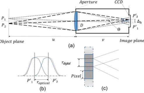
The schematic of the optical telescope is illustrated in Fig. 2 (a). An achromatic doublet lens is used to form an image on the charge-coupled device (CCD) array. The original lens of the camera, which has a short focal length, is removed. The two cameras used are generic webcams with resolution 640 x 480 pixels.
Fig. 2. Optical imaging: Achromatic doublet lens telescope design (a), optical diffraction limit (b), CCD array and digital limit (c).
[image:3.595.181.413.75.296.2] [image:3.595.175.422.482.642.2]main factors limiting the resolution (Θmin→ ∆hmin) are the pixel size on the CCD array and the optical limit
(also known as diffraction limit). These limitations are illustrated in Fig. 2 (b) and Fig. 2 (c).
The minimum resolution ∆hmin is defined as the maximum between the optical limitation (𝑟𝑜𝑝𝑡𝑖𝑐𝑎𝑙) and
digital limitation (𝑟𝑑𝑖𝑔𝑖𝑡𝑎𝑙):
∆ℎ𝑚𝑖𝑛= 𝑚𝑎𝑥 {𝑟𝑜𝑝𝑡𝑖𝑐𝑎𝑙; 𝑟𝑑𝑖𝑔𝑖𝑡𝑎𝑙} (1)
The digital limitation of the camera is characterized by the pixel size of the CCD array (𝑟𝑑𝑖𝑔𝑖𝑡𝑎𝑙 = 4 × 10⁻⁶𝑚), the focal lens and the lens diameter. The optical limitation is defined as:
𝑟𝑜𝑝𝑡𝑖𝑐𝑎𝑙 =1.22𝜆𝑓
𝐷 (2)
where λ is the average wavelength of the visible range, considering the visible range from 400 to 800 nm (λ = 600 nm), f is the focal length and D is the diameter of the lens. The system optical resolution is 𝑟𝑜𝑝𝑡𝑖𝑐𝑎𝑙 = 3.2 × 10⁻⁶𝑚 when using a 40 nm achromatic focal length with a diameter of 𝐷 = 2.22 𝑐𝑚. The minimum
angular resolution of the telescope is restricted by the optical limitation and is defined as:
𝜃𝑚𝑖𝑛= 𝑡𝑎𝑛−1(∆ℎ𝑓𝑚𝑖𝑛) ≈ 33 × 10−6 𝑟𝑎𝑑 (3)
The second camera of the telescope is used unmodified as wide field-of-view (finder-scope).
2.1.2. Telescope structure
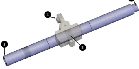
The telescope structure is assembled using 3D printed elements with polylactic acid (PLA) plastic. The thickness of the tube wall is set at 4.5 mm to ensure robustness yet keeping the structure lightweight. The tube structure (shown in Fig. 3) is divided into four parts: three parts forming the main tube (due to 3D printer size limitation) and one part to hold the telescope tube and the finder-scope. The camera used as narrow field-of-view is located at the back of the tube as illustrated in Fig. 3 (labeled 1). The lens coupled to this camera is located at the opposite side (labeled 2) at a distance equal to the focal length (40cm). The tube is held by a 3D printed structure (labeled 3 in Fig. 3). This holder is fixed to a gear allowing the elevation motion. The wider field-of-view camera is located on the top of the tube fixed in the holder structure (labeled 4).
Fig. 3. 3D printed tube mounting representation, 1) Narrow field-of-view camera position, 2) Lens, 3) Holder structure, 4) Finder-scope holder.
The tube structure is made using 3D printer due to on-site availability but regular PVC pipe can be used to lower cost of kit development.
2.1.3. Mechanical design of the telescope mounting
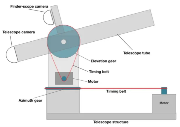
[image:4.595.176.417.514.633.2]to increase the movement precision. The first stepper motor with a timing belt is used for the elevation motion.
Fig. 4. Mechanical drawing of the telescope
The telescope with the elevation system is mounted on a rotating stage controlled by the second motor (with another timing belt for increase movement precision). In this design, timing belt and timing pulley were selected since they had negligible backlash [19]. The CAD models were designed and 3D printed using PLA filament for timing pulley and flexible filament for the two-timing belt. These timing belt are re-used from another research project available at the laboratory. In order to keep the system low-cost for productions, commercial timing belt might be a better choice. Stepper motors (ref. Nema 17, 17HS4401, Motion King, China) are used as actuator because they are low cost and high performance over torque, position, RPM and open/closed loop control strategy. The advantage of stepper motor over DC geared and servo-motor is their low-cost range (less than 20 US dollars). They have been widely used in CNC machine, 3D printer and other motion control applications [20].
2.2. System Calibration
The aim of the system calibration is to compensate for the misalignment of the telescope with the finder-scope as shown in Fig. 5. An image-processing algorithm is developed to automatically localize the telefinder-scope image onto the finder-scope image in order to facilitate the object tracking and automatic movements. The calibration process requires a set of images from both cameras with an object (celestial) visible in each frame. The algorithm determines the overlapping region of the telescope image in the finder-scope by using a template-matching technique.
[image:5.595.143.452.106.324.2] [image:5.595.152.447.610.728.2]Different template matching approaches exist to calibrate overlapping field of view from multiple cameras such as the fast-normalized cross-correlation [21], features-based algorithm [22], among others [23]. For this calibration process, template matching algorithm based on cross-correlation is used in order to find a peak of similarity between the finder-scope image and a re-scaled telescope image.
2.2.1. Dataset
The calibration process requires set of images (one from wide field-of-view, one from narrow field-of-view) taken simultaneously. Both images must contain specific feature(s) to be considered relevant. The feature used is the edge of the moon in the telescope image as it is easier to detect the overlapping of an edge rather than the center and the full moon in the viewfinder due to its large size and ease of visualization.
2.2.2. Distinct moon edge detection
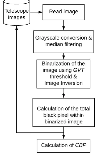
A preliminary task is to select only distinct moon edge from the acquired database. Moon images can be considered as edge images if they meet a defined ratio of pixel between the background and the moon surface. The ratio aims to select only images that match our definition of a distinctive edge. This is performed using on a two-steps algorithm shown in Fig. 6 and 7. The first part of the algorithm determines the average grayscale threshold GVT that is used to binarized images in order to get the average pixel ratio required to determine a distinct moon edge.
All images of the dataset are converted to grayscale and a median filter of size 17 is applied on the images of the finder-scope as despite special care being taken during the removal of the original lens, dust generated noise on the sensor. The image is binarized using Otsu algorithm and then inverted. The average value 𝑟𝑚𝑜𝑜𝑛 of the grayscale images is calculated using the following equation.
𝑟𝑚𝑜𝑜𝑛(𝑘) = 𝑁×𝑀1 ∑ ∑𝑀 𝐼(𝑘)𝑏𝑖𝑛(𝑛, 𝑚) × 𝐼(𝑘)𝑔𝑟𝑎𝑦(𝑛, 𝑚) 𝑚=1
𝑁
𝑛=1 (4)
where 𝑟𝑚𝑜𝑜𝑛(𝑘) represents the average of the multiplication of the Otsu binarized picture 𝐼(𝑘)𝑏𝑖𝑛, the gray-scaled converted image 𝐼(𝑘)𝑔𝑟𝑎𝑦 for an image k and (n,m) represents a pixel location.
The average gray value threshold GVT of the dataset is obtained using the following equation:
𝐺𝑉𝑇 = 𝐾1∑𝐾𝑘=1𝑟𝑚𝑜𝑜𝑛(𝑘) (5)
where K is the total number of image in the database. The second part of the algorithm presented in Fig. 7 is using GVT to binarize all images and calculates the black pixel ratio CBP which represents the minimum amount of black pixel to consider the image as containing a distinct moon edge picture and is defined as:
𝐶𝐵𝑃 = (𝐾1∑ 𝑟𝑛𝑖𝑔ℎ𝑡(𝑘)) − √∑(𝑟𝑛𝑖𝑔ℎ𝑡−𝑟̅̅̅̅̅̅̅̅̅)𝑛𝑖𝑔ℎ𝑡
2
𝐾 𝐾
𝑘=1 (6)
Fig. 6. Flow-chart GVT threshold calculation.
[image:7.595.222.386.75.418.2] [image:7.595.207.365.485.739.2]2.2.3. Rescaling factor determination
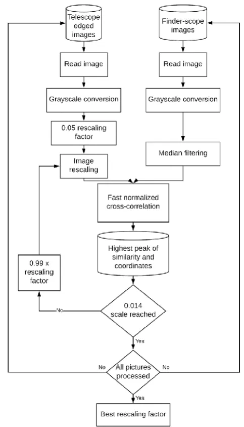
The calibration process based on cross-correlation template algorithm aims to detect the location of the targeted mask (narrow field of view image) in the finder-scope image in order to correct the mounting offset. A preliminary rescaling process is necessary before this steps as both cameras have similar resolution. This step is required in order to estimate the downsizing factor of the narrow field of view image to match its equivalent in the finder-scope image. This method (shown in Fig. 8) is based on an automatic rescaling algorithm coupled to a fast-normalized cross-correlation algorithm. The starting rescaling factor is set at 0.05 and is iteratively decreased by a factor of 0.99 until reaching the minimum limit set at 0.014 from the original size. The maximum limit gives an image of a size equal to 32 × 24 pixels. The minimum rescaling factor of 0.014 a size equal to 9 × 6 pixels. The scaling limits are empirically selected following manual rescaling in order to speed up the process.
Fig. 8. Rescaling factor calculation process.
[image:8.595.184.426.235.657.2]𝑔(𝑢, 𝑣) = ∑𝑥,𝑦[𝑓(𝑥,𝑦)−𝑓̅𝑢,𝑣][𝑡(𝑥−𝑢,𝑦−𝑣)−𝑡̅]
{∑𝑥,𝑦[𝑓(𝑥,𝑦)−𝑓̅𝑢,𝑣]2∑𝑥,𝑦[𝑡(𝑥−𝑢,𝑦−𝑣)−𝑡̅]2}
0.5 (7)
where 𝑓̅(𝑢, 𝑣) represents the mean of 𝑓(𝑥, 𝑦) region under the template and 𝑡̅ represents the mean of the template. The index 𝑔(𝑢, 𝑣) indicates the correlation coefficient calculated for a position u and v. The obtained result is a correlation coefficient between the mask and the template for each position in the mask. The highest correlation coefficient corresponds to the overlapping position of the small field-of-view within the finder-scope image. The highest peak of similarity and its coordinates are selected. It results in a rescaling factor of 0.018 from the original size giving an image with a size equal to 12 × 9 pixels. Once the rescaling factor is obtained, all images of the targeted mask are rescaled before being processed by calibration algorithm.
2.3. Offset Calibration
The flow-chart of the implemented calibration algorithm is shown in Fig. 9.
Fig. 9. Flow-chart of the calibration algorithm based on cross-correlation in Fourier domain.
[image:9.595.175.422.264.616.2]2.3.1. Fourier domain cross-correlation
Cross-correlation, 𝑔(𝑥, 𝑦), can be calculated indirectly using fast Fourier transform (FFT), where 𝐺(𝑣𝑥, 𝑣𝑦) is the direct multiplication of the Fourier transforms of the mask 𝑓(𝑥, 𝑦), and template 𝑡(𝑥, 𝑦) using the following equation:
𝐺(𝑣𝑥, 𝑣𝑦) = 𝐹𝐹𝑇. {𝑔(𝑥, 𝑦)} = 𝐹𝐹𝑇. {𝑓} × 𝐹𝐹𝑇. {𝑡∗} (8)
The cross-correlation is the inverse Fourier transform of 𝐺(𝑣𝑥, 𝑣𝑦)
𝑔(𝑥, 𝑦) = 𝐹𝐹𝑇.−1(𝑂) (9)
In a discrete form,
𝑔(𝑥, 𝑦) = ∑ ∑𝑛−1𝜔𝑚𝑗𝑝𝜔𝑛𝑘𝑞𝑂𝑗,𝑘 𝑘=0
𝑚−1
𝑗=0 (10)
Where 𝜔𝑚= 𝑒−2𝜋𝑖𝑥/𝑚, 𝜔𝑛= 𝑒−2𝜋𝑖𝑦/𝑛, i is the imaginary unit, O is the matrix of the image m by n size, j
and k are indices that run from 0 to n-1 which represents the height-1 of the image expressed in pixels. The template image is padded with zeros in order to match the mask image size. After the Fourier transform, the mask signal is multiplied with the conjugate of the template signal. The obtained result is then normalized in order to apply the inverse Fourier transform. The x and y location can be extracted from the highest peak of similarity.
2.3.2. Overlapping area calculation
Using Fourier domain cross-correlation method, locations of highest peak of similarities 𝑝(𝑙)(𝑥,𝑦) between finder-scope images l and the corresponding telescope image 𝑡𝑙, where l ∈ [1,n] and n represents the total
number of pictures detected as an edge of the Moon, can be obtained. The error distribution e of the detection is defined by the Euclidean distance between the peak similarity coordinates and the reference coordinates. The reference coordinate represents the estimation by the user of the overlapping area in order to improve its calculation. The error distribution e is defined as:
𝑒(𝑙) = (𝑅𝑒𝑓𝑋 − 𝑝(𝑙)𝑥)2+ (𝑅𝑒𝑓𝑌 − 𝑝(𝑙)
𝑦)2 (11)
Using the average 𝜇𝑒 and the standard deviation σe of the error distribution, the following equations
determine the location of the overlapping area 𝑂𝑥 and 𝑂𝑦 on X and Y axes of the image as:
𝑂𝑥 = 𝑅𝑒𝑓𝑋 − (𝜎𝑒+ 𝜇𝑒) (12)
𝑂𝑦= 𝑅𝑒𝑓𝑌 − (𝜎𝑒+ 𝜇𝑒) (13)
Once the location of the overlapping area is known, the size, expressed in pixels, can be calculated as follow:
𝑂ℎ= 𝑅𝑒𝑓𝑋 + (𝜎𝑒+ 𝜇𝑒) − 𝑂𝑥 (14)
𝑂𝑤 = 𝑅𝑒𝑓𝑌 + (𝜎𝑒+ 𝜇𝑒) − 𝑂𝑦 (15)
where 𝑂ℎ and 𝑂𝑤 are representing the height and width value of the overlapping area.
2.3. Interface and Control
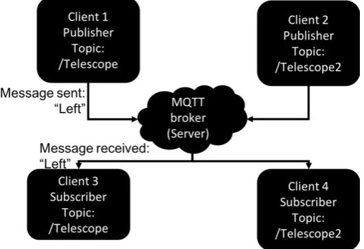
to the Raspberry Pi via general-purpose input output (GPIO) pins. Using this configuration, the azimuth (vertical axis) and the elevation (horizontal axis) movements can be controlled by the system. The Internet connectivity allows the communication between the user and the system. The remote control is based on Message Queue Telemetry Transport (MQTT) [25] communication protocol. This protocol is part of the Internet of Things technology (IOT) using the publish-subscribe pattern. An MQTT server, also called a broker, allows different channels where each client can listen (subscriber) or send (publisher) information. The MQTT protocol procedure is shown in Fig. 10.
Fig. 10. Message Queue Telemetry Transport communication protocol for multiple telescope interaction with telescope control example shown (left displacement sent and received by telescope1).
In order to control the telescope motors and to stream cameras feeds, a server-side software developed in Java is running on the Raspberry Pi. It analyzes data sent from the user on the MQTT channel corresponding to the telescope. These data are basic messages, which the server-side software analyses before performing an action.
2.4. Client
The telescope control is done through in-house software developed in Java. It allows camera feeds display, communication with the MQTT server, motors settings in order to define the movement step. It also allows image acquisition from both cameras.
3.
Results
In this section, the results of the fabrication process, the optical design and cameras calibration are presented.
3.1. Fabrication
Fig. 11. Picture of the mounted telescope with all its components
3.2. Optical Design
As presented in the section 2.1.1, the theoretical minimum angular resolution 𝜃𝑚𝑖𝑛 is defined as 𝜃𝑚𝑖𝑛= 33 × 10−6 𝑟𝑎𝑑. To estimate the angular resolution of the presented optical telescope, a manual stitched
image of the Moon (obtained from a total of 13 telescope frames) is used. The diameter of the Moon in the image is estimated as 𝑑𝑝𝑖𝑐= 1674 pixels. Assuming a perfect spherical shape of the Moon, the pixel
resolution 𝛿𝑥 on the Moon surface is defined as:
δ𝑥 =𝜋×𝑅𝑑
𝑝𝑖𝑐=
5457
1674≈ 3.26 𝑘𝑚 (16)
where R represents the radius of the Moon in kilometers. A pixel on the reconstituted image of the moon represents 3.26 km on the Moon surface. From this result, the angular resolution θ of the system is calculated as:
𝜃 =δ𝑥
𝑍 =
3.26
376292≈ 8.7 × 10⁻⁶ 𝑟𝑎𝑑 (17)
where Z is the distance between the Earth surface and the Moon surface in kilometers. It is calculated as the distance between the Earth and the Moon (384,400 km) minus the radius of the Earth (6,371 km) minus the radius of the Moon (1,737 km). The estimated angular resolution and measured one are in the same order of magnitude. The difference 𝜃𝑑𝑖𝑓𝑓 = 𝜃𝑚𝑖𝑛 − 𝜃 = 24 × 10−6 can be attributed to a shift in the estimation of
the diameter of the Moon in pixels. It is possible to calculate the minimum number of frames needed to reconstruct the complete surface as ≈ 𝐴𝑚𝑜𝑜𝑛
𝐴𝑓𝑟𝑎𝑚𝑒 , where 𝐴𝑚𝑜𝑜𝑛 is the number of pixels covering the moon
surface and 𝐴𝑓𝑟𝑎𝑚𝑒 is the total number of pixels for a frame. The estimation of 𝐴𝑚𝑜𝑜𝑛 is determined using:
𝐴𝑚𝑜𝑜𝑛 ≈ 𝜋 × 𝑟2= 𝜋 × 8372 (18)
𝐴𝑚𝑜𝑜𝑛 = 2.2 × 106 pixels2 (19)
where r is the estimated radius of the Moon on the reconstructed picture. For 𝐴𝑓𝑟𝑎𝑚𝑒, the surface can be calculated by multiplying the width (w= 640) and height (h= 480) of a frame where 𝐴𝑓𝑟𝑎𝑚𝑒 = 0.307 × 106pixels2. Using this configuration, N is defined by:
𝑁 ≈ 𝐴𝑚𝑜𝑜𝑛
3.3. Cameras Calibration
The results for the cameras calibration process show first the result of the automatic resizing algorithm, then the cross-correlation process for the definition of the overlapping area.
3.3.1. Database acquisition
The database used for the calibration process was acquired by manually controlling the orientation of the telescope using the developed application. The Moon is selected as the distant target to be visible on both cameras (finder-scope and small field of view). Using manual control, a set of 553 dual images has been collected on June 12th 2018.
3.3.2. Distinct moon edge detection algorithm
The calibration algorithm is applied on the acquired dual images from the database. After processing the database, an average ratio of 7% of black pixel in the image is required to consider the image as containing a distinct moon edge. Based on this criterion, only 432 of the 533 images satisfied this requirement.
3.3.3. Rescaling factor definition
The implemented automatic resizing algorithm using fast normalized cross-correlation defines the best rescaling factor for the calibration process. The algorithm starts at a factor set at 0.05 until 0.014 of the original size with a step multiplying the resizing factor by 0.99 after each iteration. In each edge-picture, the large field-of-view image was rescaled at different factors and the cross-correlation result (with the corresponding finder-scope image) was recorded as shown in Fig. 12 shows the cross-correlation result with the highest similarity ration. For visual purpose, only a selected number of rescaling factors are shown in the figure.
Fig. 12. Automatic rescaling factor results showing the highest cross-correlation coefficient depending on the rescaling factor.
The highest peak of similarity is detected at a rescaling factor of 0.018 as shown in the figure. Using this rescaling factor, the size of the small field of view image is reduced to 12 × 9 pixels.
3.3.4. Cross-correlation results
Fig. 13. Histogram of the similarity detection locations obtained from the cross-correlation operating in Fourier domain.
The obtained results give an overlapping area of 12 × 10 pixels with a standards deviation equal to σx =
5.76 and σy = 5.18 pixels.
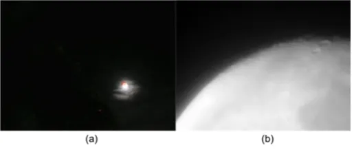
The overlapping area is a region in the large field-of-view image (finder-scope) within which the celestial object needs to be placed in order to be visible with the telescope camera. The overlapping area resulting from the Fourier domain cross-correlation is shown by a red square in Fig. 14 (a) and Fig. 14 (b) represents the picture taken at the same time with the telescope camera.
Fig. 14. Representation of the overlapping area by a red square on a finder-scope-image (a); Telescope image associated to this finder-scope image (b).
Using the calibration algorithm with the use of the cross-correlation operating in Fourier domain, 81.15% of the edged detected pictures are located within the overlapping area where others are detected outside the overlapping area with an average offset on X and Y axis equal to 5 pixels. From these results, it is possible to conclude with a good calculation of the overlapping area.
4.
Discussion
[image:14.595.170.428.405.514.2]5.
Conclusion
The presented system offers an optical digital telescope coupled with a motorization based on 3D printed structure and standard webcams making it a low-cost system. The optical system of the telescope combined the use of off-shell web-cameras where the basic lens is removed and a lens with a focal length equal to 40 cm coupled with an achromatic doublet to correct the chromatic aberration which provides a highly magnified image. Using this lens, the angular resolution is equal to 8.7 × 10⁻⁶ rad which provides a need for 8 frames to cover the Moon. The second web-camera is placed on the top of the tube in order to be used as finder-scope with a large field-of-view image. A calibration process using cross-correlation in Fourier domain is developed to determine the offset location of the telescope image in the finder-scope image. The calibration results in a calculated overlapping area with a size set as 12 × 9 pixels using 533 dual-images set. The overlapping set the position of a celestial object to be located on the large field-of-view camera in order to be seen on the telescope camera.
Acknowledgements
The authors would like to acknowledge the support from Bangkok University Scholarship.
References
[1] C. R. Kitchin, “Modern small telescope design,” in Telescopes and Techniques, Undergraduate Lecture Notes in Physics. New York: Springer Science Business Media, 2013, pp. 59–65.
[2] J. Cheng, The Principles of Astronomical Telescope Design. New York: Springer, 2010.
[3] J. M. Marr, R. L. Snell, and S. E. Kurtz, Fundamentals of Radio Astronomy: Observational Methods. CRC Press, 2015, pp. 21–24.
[4] T. A. Rector, Z. G. Levay, L. M. Frattare, J. English, and K. Pu’uohau–Pummill, “Image–processing techniques for the creation of presentation–quality astronomical images,” The Astronocical Journal, vol. 133, no. 2, pp. 598–611, 2007
[5] K. K. Arcand, M. Watzke, T. Rector, Z. G. Levay, J. DePasqualeand, and O. Smarr, “Processing color in astronomical imagery,” Studies in Media and Communication, vol. 1, no. 2, pp. 25–34, 2013.
[6] M. Serra, M. Curetti, S. G. Bravo, and L. Math, “Implementation of control algorithm for optical tracking system in Meade LX200–ACF Telescope,” in 2017 XVII Workshop on Information Processing and Control (RPIC), Mar Del Plata, Argentina, 2017, pp. 1-6.
[7] Celestron. (2018). Sky Align Technology. [Online]. Available:
https://www.celestron.com/pages/skyalign-technology [Accessed: Aug. 1, 2018].
[8] A. J. Castro–Tirado, “Robotic autonomous observatories: A historical perspective,” Advances in Astronomy, pp. 8, 2010.
[9] T. F. Slater, A. C. Burrows, D. A. French, R. A. Sanchez, and C. B. Tatge, “A proposed astronomy learning progression for remote telescope observation,” Journal of College Teaching & Learning, vol. 11, no. 4, pp. 197–2006, 2014.
[10] T. M. Brown, N. Baliber, F. B. Bianco, M. Bowman, B. Burleson, P. Conway, M. Crellin, E ́ .Depagne, J. DeVera, B. Dilday, D. Dragomir, M. Dubberley, J. D. Eastman, M. Elphick, M. Falarski, S. Foale, M. Ford, B. J. Fulton, J. Garza, E. L. Gomez, M. Graham, R. Greene, B. Haldeman, E. Hawkins, B. Haworth, R. Haynes, M. Hidas, A. E. Hjelstrom, D. A. Howell, J. Hygelund, T. A. Lister, R. Lobdill, J. Martinez, D. S. Mullins, M. Norbury, J. Parrent, R. Paulson, D. L. Petry, A. Pickles, V. Posner, W. E. Rosing, D. J. Sand, E. S. Saunders, J. Shobbrook, A. Shporer, R. A. Street, D. Thomas, Y. Tsapras, J. R. Tufts, S. Valenti, K. Vander Horst, Z. Walker, G. White, and M. Willis, “Las Cumbres Observatory global telescope network,” Publications of the Astronomical Society of the Pacific, vol. 125, no. 931, pp. 1031– 1055, 2013.
[11] Telecope Organisation, “OpenScience Observatories,” [Online]. Available: http://telescope.org [Accessed: Jun. 8, 2018].
[13] P. M. Sadler, R. R. Gould, P. S. Leiker, P. R. A. Antonucci, R. Kimberk, F. S. Deutsch, B. Hoffman, M. Dussault, A. Contos, K. Brecher, and L. French, “MicroObservatory Net: A network of automated remote telescopes dedicated to educational use,” Journal of Science Education and Technology, vol. 10. no. 1, pp. 39–55, 2001.
[14] E. L. Gomez and M. T. Fitzgerald, “Robotic telescopes in education,” Astronomical Review, vol. 13 no. 1, pp. 2821–68, 2017.
[15] M. Wrigley, “Welcome to PiKoN,” PiKonic, 2017. [Online]. Available: https://pikonic.com [Accessed: Jul. 10, 2017].
[16] Hanna Watkin, “3D printed telescope: PiKoN Kits now available to buy | All3dp,” [Online]. Available: https://all3dp.com/pikon-3d-print-raspberry-pi-astro-cam/ [Accessed: Feb. 13, 2019].
[17] 3dexperiencelab, “Ultrascope | Dassault Système®,” [Online].
https://3dexperiencelab.3ds.com/en/projects/iot/ultrascope/ [Accessed: Feb. 13, 2019].
[18] O. S. Agency, “UltraScope –Open Space Agency,” [Online]. Available: http://www.openspaceagency.com/ultrascope/ [Accessed: Jun. 8, 2018].
[19] R. Perneder and I. Osborne, Handbook Timing Belts: Principles, Calculations, Applications. Springer Science & Business Media, 2012.
[20] Machinetoolhelp, “Advantages & Disadvantages of Stepper motors & DC servo motors,” [Online]. Available: http://www.machinetoolhelp.com/ Automation/systemdesign/stepper dcservo.html. Accessed on: Aug. 1, 2018.
[21] K. Briechleand AND U. D. Hanebeck, “Templatematchingusingfastnormalized cross correlation,” in Optical Pattern Recognition XII, Proc. SPIE 4387, 2001, pp. 8.
[22] D. G. Lowe, “Distinctive image features from scale-invariant key-points,” Int. J. Comput. Vis., vol. 60, no. 2, pp. 91–110, 2004.
[23] R. Brunelli, Template Matching Techniques in Computer Vision: Theory and Practice. John Wiley & Sons, 2009. [24] J. P. Lewis, “Fast template matching,” Vision Interface, vol. 95, pp. 120–123, 1995.
[25] U. Hunkeler, H. L. Truong, and A. Stanford-Clark, “MQTT-S A publish/subscribe protocol for Wireless Sensor Networks,” in 2008 3rd International Conference on Communication Systems Software and Middleware