Essays on Robust Model Selection and Model Averaging for Linear Models

(1)

Essays on Robust Model Selection and

Model Averaging for Linear Models

Le Chang

May 2017

(2)

(3)

(4)

(5)

Declaration

I hereby declare the work in this thesis is my own except where otherwise stated. Any contribution made to the research by others, with whom I have worked at the Australian National University (ANU) or elsewhere, is explicitly acknowledged in the thesis.

(6)

(7)

Acknowledgements

This thesis emerges from my Ph.D program, funded by the Research School of Finance, Actuarial Studies and Statistics (RSFAS) at the ANU. During my three year Ph.D program, I have been helped by many individuals and institutions. I would like to express my gratitude to those who made this thesis possible.

First of all, I would like to take this opportunity to thank all of my supervisors, Professor Steven Roberts, Professor Alan Welsh, and Dr Yanrong Yang, whose continuous assistance, guidance and encouragement throughout this period have been paramount to the completion of this thesis. I particularly thank Professor Steven Roberts for his continuous guidance throughout all the stages of my Ph.D study. His enthusiastic support has made my Ph.D experience productive and stimulating. I sincerely thank Professor Alan Welsh for providing his expertise in many fields of statistics. His wide knowledge and expert thinking have been of great value to me. I also gratefully acknowledge Dr Yanrong Yang for her timely feedback and kind discussions on the last chapter of my thesis. Her end-less patience in supervising me to pursue the excellence has been crucial to the completion of my thesis.

I would like to express special thanks to the RSFAS for providing me with an excellent academic environment and generous funding throughout my Ph.D program. In particular, I would like to thank Associate Professor Timothy Hig-gins, the Ph.D Convenor in Statistics and the Director in Higher Degree Research of RSFAS, for providing me with considerable assistance in Ph.D-related issues. Moreover, I am grateful to Associate Professor Stephen Sault and Ms Tracy

(8)

ner for their effort to arrange my tutorials.

Doctoral research at the ANU has been a memorable experience for me, and I would like to thank the exceptional RSFAS faculty staff for their academic support and general help. Additionally, thanks to my fellow PhD students of RSFAS, my PhD study has been enjoyable and fruitful.

Finally, I owe a great debt to my mother Yuxiang Li and father Zhaoping Chang. Thank you for your endless love and support. I especially thank Hailun Zhou, who provided me with unconditional companionship, patience and moral support throughout my Ph.D. This work is dedicated to my family.

(9)

Abstract

Model selection is central to all applied statistical work. Selecting the variables for use in a regression model is one important example of model selection. This thesis is a collection of essays on robust model selection procedures and model averaging for linear regression models.

In the first essay, we propose robust Akaike information criteria (AIC) for MM-estimation and an adjusted robust scale based AIC for M and MM-MM-estimation. Our proposed model selection criteria can maintain their robust properties in the presence of a high proportion of outliers and the outliers in the covariates. We compare our proposed criteria with other robust model selection criteria discussed in previous literature. Our simulation studies demonstrate a significant outper-formance of robust AIC based on MM-estimation in the presence of outliers in the covariates. The real data example also shows a better performance of robust AIC based on MM-estimation.

The second essay focuses on robust versions of the “Least Absolute Shrinkage and Selection Operator” (lasso). The adaptive lasso is a method for performing simultaneous parameter estimation and variable selection. The adaptive weights used in its penalty term mean that the adaptive lasso achieves the oracle property. In this essay, we propose an extension of the adaptive lasso named the lasso. By using Tukey’s biweight criterion, instead of squared loss, the Tukey-lasso is resistant to outliers in both the response and covariates. Importantly, we demonstrate that the Tukey-lasso also enjoys the oracle property. A fast accelerated proximal gradient (APG) algorithm is proposed and implemented for

(10)

computing the Tukey-lasso. Our extensive simulations show that the Tukey-lasso, implemented with the APG algorithm, achieves very reliable results, including for high-dimensional data wherep > n. In the presence of outliers, the Tukey-lasso is shown to offer substantial improvements in performance compared to the adaptive lasso and other robust implementations of the lasso. Real data examples further demonstrate the utility of the Tukey-lasso.

In many statistical analyses, a single model is used for statistical inference, ignoring the process that leads to the model being selected. To account for this model uncertainty, many model averaging procedures have been proposed. In the last essay, we propose an extension of a bootstrap model averaging approach, called bootstrap lasso averaging (BLA). BLA utilizes the lasso for model selec-tion. This is in contrast to other forms of bootstrap model averaging that use AIC or Bayesian information criteria (BIC). The use of the lasso improves the com-putation speed and allows BLA to be applied even when the number of variables

(11)

List of Abbreviations

AIC Akaike information criteria

APG Accelerated proximal gradient

BIC Bayesian information criteria

BLA Bootstrap lasso averaging

BMA Bayesian model averaging

FMA Frequentist model averaging

FR Forward regression

IRLS Iteratively reweighted least squares

LAD Least absolute deviation

LASSO Least Absolute Shrinkage and Selection Operator

LMS Least median of squares

LQA Local quadratic approximation

LTM Least trimmed sum of squares

MAD Median absolute deviation

MSPE Mean squared prediction error

NIR Near-infrared

(16)

OLS Ordinary least squares

SIS Sure independence screening

(17)

Chapter 1 Introduction

Model selection is central to all applied statistical work. Selecting the variables for use in a regression model is one important example. Over the past two decades, a number of different model selection approaches have been rapidly developed and there exists a substantial literature that addresses the issue of methods for model selection.

Stepwise procedures (sequential testing), allowing variables to be added or deleted at each step, have often been employed. However, such testing schemes based on p values only compare two nested models and have been widely criti-cized since hypothesis tests generally form a very poor basis for model selection (Akaike, 1974). Cross-validation and its variations have been suggested and dis-cussed as useful model selection methods (Mosteller and Tukey, 1968; Shao, 1993). However, these methods are quite computer intensive and tend to be impracti-cal if a large number of models need to be evaluated (Burnham and Anderson, 2004). The adjusted coefficient (Draper and Smith, 1981) and Mallow’s Cp statis-tic (Mallows, 1973) are also widely used in least square regression and provide a ranking of all candidate models.

The general approach that is the focus of the first essay is the model selection methods that choose models by minimizing an expression (criterion) that can be written as a loss term in addition to a penalty term. More specifically, these model

(18)

selection criteria, such as the Akaike information critera (AIC) (Akaike, 1974), the Bayesian information criteria (BIC) (Hoeting et al., 1999) and their variations will be considered. Most of these prevalent model selection criteria are based on the squared loss, yet it is well known that the commonly used squared loss function is very sensitive to outliers and other violations to the normality assumption for error distribution. A growing body of literature is concerned with the model selection procedures for linear models that are less sensitive to outliers: a robust Cp (Ronchetti and Staudte, 1994), a robust version of cross-validation (Ronchetti et al., 1997), and weighted versions of likelihood estimators (Agostinelli, 2002). Ronchetti (1985) proposes a robust version of AIC for M-estimation by replacing the squared loss with Huber’s function. However, Huber’s loss can only be robust to outliers in the response values. Outliers in the covariates also appear frequently and they generally have a greater effect on the accuracy of the regression estimates than the outliers in the response. In the first essay, we propose to replace the loss function by Tukey’s biweight criterion and develop a robust AIC based on MM-estimation that copes with outliers in both the response and the covariates.

(19)

3

penalty into an L1 penalty. The lasso not only shrinks some coefficients, achiev-ing a better prediction, but also sets others to zero and hence offers parsimonious solutions to ease the interpretation.

Over the last few decades, the lasso has become a very popular technique for simultaneous estimation and variable selection. A significant volume of literature further investigated the properties of the lasso estimates and developed different versions of the lasso. Zou (2006) stated that there exist certain scenarios where the lasso is inconsistent for variable selection and therefore he suggests the adap-tive lasso where adapadap-tive weights are used for penalizing different coefficients in the L1 penalty. The adaptive lasso enjoys the oracle properties as it performs as well as the true underlying model asymptotically. However, as mentioned pre-viously, datasets with outliers are commonly encountered in statistical analysis. These outliers may appear in the response and/or the predictors. The lasso es-timates, which utilize ordinary least squares (OLS), also suffer from the effect of outliers. Some authors have considered robust versions of the lasso, generally uti-lizing penalized versions of M-estimators, as in Owen (2007), Wang et al. (2007), Li et al. (2011), and in Lambert-Lacroix and Zwald (2011). Wang et al. (2007) proposed to overcome the presence of outliers by combining the least absolute deviation (LAD) loss with the lasso penalty. Unfortunately, it is well known that the LAD loss is not adaptable for small errors because it strongly penalizes small residuals (Owen, 2007; Lambert-Lacroix and Zwald, 2011). In other words, the LAD-Lasso has lower efficiency than OLS estimates when there are no outliers in the response. Owen (2007) and Lambert-Lacroix and Zwald (2011) preferred to replace the squared loss with Huber’s loss, a hybrid of the squared error and absolute error loss functions.

(20)

the method the Tukey-lasso for handling outliers in the response and covariates. In our simulation study, we show that the Tukey-lasso outperforms the adaptive lasso and other robust implementations of the lasso, particularly in the presence of outliers in both the response and the predictors. We further propose an ac-celerated proximal gradient (APG) algorithm to compute the Tukey-lasso. The APG computes the lasso minimization problem and guarantees a global minimizer for a convex objective function. Although the objective function for the robust lasso with Tukey’s biweight is non-convex, the APG algorithm still achieves very reliable results (a local minimizer) when the starting value of the algorithm is carefully selected.

(21)

5

Among these papers contributing to model averaging, the most relevant work for our third essay is bootstrap model averaging first proposed by Buckland et al. (1997). Bootstrap model averaging in Buckland et al. (1997) utilizes the bootstrap to generate resamples, applies the model selection criteria independently to each resample and further computes the weights assigned to each model. However, similar to the traditional model selection procedures by AIC or BIC, bootstrap model averaging is computationally intensive with a large number of variables and computationally infeasible with the number of variables greater than the sample size. In this third paper, we modify bootstrap model averaging by utilizing the lasso (Tibshirani, 1996) as a model selection tool, instead of the traditional AIC or BIC, to improve the computation speed and realize the computational feasibility even when the number of variables p is larger than the sample size n. We call this modified version of bootstrap model averaging, ‘bootstrap lasso averaging’.

(22)

(23)

Chapter 2 A Comparison of Robust Model

Selection Criteria Based on M

and MM-estimators

2.1 Introduction

It is well known that the commonly used least square estimators in the linear re-gression setting are very sensitive to outliers and other violations to the normality assumption for error distribution. Various types of robust estimators have been introduced and discussed, such as M-estimator, S-estimator, and MM-estimator (Huber, 2011; Hampel, 1971; Yohai, 1987). However, the presence of outliers not only affects these estimators, but also (and more severely) the model selection procedures, especially these likelihood based criteria (AIC, BIC, and Mallow’s Cp) (Ronchetti et al., 1997). An increasing volume of literature is concerned with the model selection procedures for linear models that are less sensitive to outliers: a robust Cp (Ronchetti and Staudte, 1994), a robust version of cross-validation (Ronchetti et al., 1997), and weighted versions of likelihood estimators (Agostinelli, 2002). Ronchetti (1985) proposed a robust version of AIC for M-estimation by replacing the squared loss with a general function ρ (e.g. Huber’s

(24)

function). However, M-estimation and Huber’s loss can only be robust for outliers in the response values. Outliers in the covariates also appear frequently and they generally have a greater effect on the accuracy of the regression estimates than the outliers in the response. To be robust against outliers in both the covariates and the response, the derivative of the loss function needs to be redescending (Rousseeuw, 1984; Yohai, 1987). A commonly used loss function with this prop-erty is Tukey’s biweight (Tukey, 1960). In this work, we propose to replace the loss function by Tukey’s biweight criterion and develop a robust AIC based on MM-estimation that copes with outliers both in the response and the covariates.

(25)

2.2. ROBUST ESTIMATION 9

The purpose of this chapter is to investigate and compare the selection proba-bilities for several robust model selection criteria, and to ascertain, the prediction ability of the best model selected by these criteria.

2.2 Robust estimation

2.2.1 Linear regression model

Linear regression is the most commonly used approach to model the relation-ship between a dependent variable and one or more independent variables. We consider the linear regression model,

yi =XiTβ+i, i= 1,2, . . . , n, (2.1)

whereyi is the response variable on theithobservation,Xi = (1, xi1, xi2, . . . , xip)T are the values of the covariates for theith _observation, _p_{is the number of} covari-ates, β = (β0, β1, β2, . . . , βp)T are coefficient parameters, and i, i = 1,2, . . . , n, is an independently normally distributed random variable with mean zero and variance σ2.

The estimates of β are usually obtained by the method of ordinary least squares (OLS). The OLS estimate is the solution to the problem:

b

βLS = argmin n X

i=1

yi−XiTβ 2

. (2.2)

Unfortunately, the use of the OLS method would be inappropriate for use in a problem containing outliers or extreme observations. When there are outliers in the data, the summation part of the above minimization problem is dominated by the residual squares of these extreme observations. In such a situation, the OLS estimators often perform very poorly.

(26)

im-portant tool for analyzing data that are heavily affected by the outliers and it provides results that are resistant to outliers. Some of the well-known robust regression methods are M-estimation, S-estimation, and MM-estimation.

2.2.2 M-estimation

M-estimation is the most general method of robust regression, introduced by Hu-ber et al. (1964). The letter ‘M’ indicates that it is an estimator of the maximum likelihood type. If we still consider the linear model as described in (2.1), the M-estimator minimizes the objective function,

b

βM = argmin n X

i=1

ρ

yi−XiTβ

σ

. (2.3)

Compared with the OLS method, the squared residual function is now replaced by another function, which is a symmetric, non-decreasing in [0,+∞), and with

ρ(0) = 0. Moreover, to be more robust against outliers that result in large residuals, this ρ function should increase less for large values of residuals than the squared function in the OLS. An optimal choice of ρ is provided by Huber’s family with a loss function,

ρc(u) =   

u2

2 if |u| ≤c

c|u| − c2

2 otherwise,

(2.4)

where c is a tuning constant that controls the level of robustness and a stan-dard choice of c is c = 1.345 for 95% asymptotic efficiency in standard normal distribution.

To minimize the objective function as in (2.3), we differentiate it with respect to the coefficients β, set the partial derivatives to 0, and obtain a system of estimating equations for the coefficients,

n X

i=1

ψc

yi−XiTβ

σ

(27)

2.2. ROBUST ESTIMATION 11

where ψc is the derivative of ρc. Further, σ could be estimated by the median absolute deviation (MAD) of the residuals, MAD = 1.4826×Mediani=1,...,n(|ri|), or by Huber’s proposal 2 (Huber, 2011).

Solving the estimation equations is a weighted least squares problem and in most cases, the iteratively reweighted least squares (IRLS) algorithm could be performed, which is typically the preferred method. In this work, we estimate the regression parameters using the ‘rlm()’ function from the ‘MASS’ package in R using method of ‘M’.

2.2.3 S-estimation

Although M-estimation could be resistant to outliers in response values and achieve high asymptotic efficiency, M-estimators are not robust against high lever-age points (outliers in covariates), and more importantly, have a disappointing breakdown property. The breakdown point of an estimator is the proportion of ‘bad’ data that can be arbitrarily large values without making the estimator arbitrarily bad.

The first estimators with high breakdown points are the least median of squares (LMS) and the least trimmed sum of squares (LTM). A more general class of high breakdown estimators that likewise do not suffer from leverage points is introduced by Rousseeuw and Yohai (1984), and is known as the class of scale-type or S-estimators (Salibian-Barrera and Yohai, 2006).

The S-estimator is defined byβb_S = argmin b

σ(β) with a determining minimum robust scale estimator and the scale function satisfies the equation,

1

n

n X

i=1

ρ

yi−XiTβ b

σ(β)

=K, where K = Z

ρ(z)φ(z)dz. (2.6)

(28)

ρd(u) =     

d2

6

1−h1− u d

2i3

if |u| ≤d

d2

6 if |u| ≥d

(2.7)

The solution to the S-estimator could also be found by using an IRLS method. The choice of d= 1.548 yields K = 0.5, indicating that the S-estimator achieves a 50% breakdown point. The S-estimator has much higher breakdown point than the M-estimator when its ψ function redescends, where ψ is the derivative of

ρ. However, a high breakdown point generally results in a low efficiency. When the S-estimator described above obtains a 50% breakdown point, it only achieves 28.7% efficiency at the core model with a standard normal distribution.

2.2.4 MM-estimation

It is possible to have both high breakdown point and high efficiency. This is achieved by MM-estimation, a three-stage procedure introduced by Yohai (1987). In the first stage, an initial regression estimate (e.g. LMS) is computed with high breakdown point but is not necessarily efficient. In the second stage, an M-estimation of the errors scale is calculated based on the initial estimate (the first M). In the third stage, an M-estimate of regression coefficients is computed based on the scale estimate obtained in the second stage (the second M). Briefly speak-ing, the MM-estimator is computed as an M-estimator starting at the coefficients provided by a high breakdown S-estimator and using the fixed scale afforded by the S-estimator. As mentioned by one of the referees, another robust estimator,

τ-estimator (Yohai and Zamar, 1988), also combines good robustness and high efficiency. However, we only focus on a more widely used MM-estimator in this chapter.

If we defineρd0 to be the ρ function as in the S-estimation procedure andρd1

to be the ρ function as in the M-estimation of the third stage, ρd1 should satisfy

ρd1(u)≤ρd0(u) for all u ∈R and supρd1(u) = supρd0(u). MM-estimator is then

(29)

2.3. ROBUST MODEL SELECTION CRITERIA 13

b

βM M = argmin n X

i=1

ρd1

yi−XiTβ b

σs

, (2.8)

where ρd1 is still the Tukey’s biweight function mentioned in S-estimation.

How-ever, a larger value of dis chosen andd= 4.685 is a typical choice ford. Further,

b

σs is the S-scale estimator, which was derived in the S-estimation procedure by using ρd0 as theρ function.

Again, to solve the above equation, we could differentiate the objective func-tion with respect to the coefficientsβand set the partial derivatives to 0, obtain-ing a system of estimatobtain-ing equations for the coefficients,

n X

i=1

ψd1

yi−XiTβ b

σs

X_iT =0 (2.9)

where ψd1 is the derivative of ρd1 and an IRLS algorithm could be applied to

find the solution to this equation. With d = 4.685, the MM-estimator achieves 95% efficiency at standard normal distribution and the 50% breakdown point. Therefore, it is a superior estimator to either the M-estimator or the S-estimator, in terms of breakdown point and efficiency. Here, we estimate the MM-regression parameters using the ‘rlm()’ function from the ‘MASS’ package in R using method of ‘MM’.

2.3 Robust model selection criteria

Model selection is a key component of all statistical work with data. Selecting the variables for use in a regression model is one important example. Using all variables in the model suffers from high variability in parameter estimation, and thus, results in a very poor prediction accuracy. Over last few decades, various model selection criteria have been rapidly developed. Among these model selec-tion criteria, AIC (Akaike, 1974) is increasingly used for all statistical analysis.

(30)

out-liers or to other departures from normality assumptions in the error distribution. Therefore, model selection procedures require special care in the presence of out-liers. A growing number of papers are concerned with model selection procedures for linear models that are less sensitive to outliers: Ronchetti (1985); Ronchetti and Staudte (1994); Ronchetti et al. (1997); Agostinelli (2002); Tharmaratnam and Claeskens (2013); M¨uller and Welsh (2005). In this section, we will introduce the six different types of model selection criteria considered in our analysis and comparison.

2.3.1 Classical AIC

AIC (Akaike, 1974), a variant of the Kullback-Leibler divergence between the true model and the approximating candidate model, has been widely used as a model selection tool over the past decades. According to Ronchetti (1985), if we consider a linear regression model in Section 2.2 and assume that the errors follow some distribution with density g, a generalized AIC proposed by Bhansali and Downham (1977) for a given fixed α is

AIC(p;α) = −2 n X

i=1

logg yi−X

T i βb b

σ

!

+αp+K(n,_bσ), (2.10)

whereK(n,_bσ) is a function ofn and_bσ,_bσis an estimate ofσ, andpis the number of parameters in the linear regression model. When g is a standard normal distribution and the choice of α isα= 2, AIC(p; 2) is reduced to the well-known criterion, Mallows’Cp, proposed by Mallows (1973),

Cp = n X

i=1

yi −XiTβb b

σ

!2

−n+ 2p. (2.11)

Further, when σ_b is the maximum likelihood estimate of σ, this criterion re-duces to the traditional AIC for linear regression,

(31)

whereσ_bM L is the maximum likelihood estimate ofσ. Further, it is widely known that Cp is asymptotically equivalent to the traditional AIC. However, it could be noted that AIC and its variant, Cp are based on the normality assumption of error distribution and they are sensitive to outlying observations. In the pres-ence of outliers, Pn_i₌₁yi−XiTβb

b σ

2

is dominated by the residuals of these extreme observations. In this situation, AIC or Cp performs poorly. Therefore, we search for more robust alternatives.

2.3.2 Robust AIC for M-estimation

Ronchetti (1985) proposed a robust version of AIC for M-estimation by replacing logg with a more general functionρ,

RAIC.M = 2 n X

i=1

ρ yi−X

T i βb_M b

σ

!

+αp, (2.13)

where in this case,βb_M is the M-estimator as in Section 2.2,_bσis a robust estimate of σ and does not change from model to model. The model with the smallest value ofRAIC.M is selected as the best model. As discussed in Ronchetti (1985), the extension of AIC to a more robust version of itself is the exact counterpart of the maximum likelihood estimation for M-estimation.

Another issue we address here is the choice of parameter α. Following the results of Stone (1977), the penalty term αp= 2 trace(M−1_Q_{), where}

M =−E

∂ψ ∂β

=Eψ0xxT, Q=Eψψ2 =Eψ2xxT.

Here, ψ is the derivative of ρ with respect to coefficient parameters. Ronchetti (1985) suggests that M = E

ψ0xxT

= E[ψ0]·E[xxT_{] and} _Q ₌ _E

ψ2_xxT =

E[ψ2_]_·_E_[_xxT_{]. Thus, the penalty term is}

αp= 2 trace(M−1Q) = 2E[ψ

2_]

(32)

Here, the choice ofαis 2E_E[_[ψ_ψ20_]]. Thisα is then fixed across all the possible models.

When the ρ function is simply a square function (as in the case of OLS), αp is exactly equal to 2p and the selection criterion RAIC.M simply reduces to the traditional AIC (or its variant, Cp).

Therefore, in this work, we compute robust version of AIC for M-estimation suggested by Ronchetti (1985) as,

RAIC.M = 2

n X

i=1

ρc

yi−XiTβb_M b

σ

!

+ 2E[ψ

2

c]

E[ψ0 c]

p (2.15)

whereρcis the Huber’s function,βb_M is the M-estimator, b

σ is the median absolute deviation (MAD) of the residuals from the full model, and E[ψ2

c] and E[ψ 0 c] are estimated respectively by the average of the empirical values of ψ2

c and ψ 0 c from the full model.

2.3.3 Robust AIC for MM-estimation

It is widely known that M-estimators have a low breakdown point. Since the robust version of AIC based on M-estimation applies the same ρ function (the Huber function) as the M-estimators, it loses its robust property in the presence of a high proportion of outliers. More importantly, in regression analysis, M-estimation is only robust to the outliers in the response but not the outliers in the covariates.

Yohai (1987) proposed an MM-estimation, that utilizes the S-scale estimator in an M-estimation equation and is robust to outliers in both the response and the covariates. A corresponding robust version of AIC could also be further derived based on MM-estimation. Therefore, we propose a new robust version of AIC based on MM-estimator, which obtains a higher breakdown point than the M-estimator and copes with outliers in both the response and the covariates,

RAIC.M M = 2 n X

i=1

ρd

yi−XiTβb_{M M} b

σ

!

+ 2E[ψ

2

d]

(33)

where ρd is the Tukey’s biweight function, and bσ is the MAD of the residuals of the full model by MM-estimation. The structure of RAIC.M M is similar to RAIC.M, as suggested by Ronchetti (1985). However, the loss function is replaced by the Tukey’s biweight function (ρd) and high breakdown estimators, MM-estimators (βb_{M M}) are used instead of M-estimators. In our simulation study, we find that RAIC.M M performs significantly better than RAIC.M when the proportion of outliers in the response reaches 20% or when outliers are present in the covariates.

2.3.4 Robust AIC with a prediction loss part

Robust versions of AIC for both M-estimation and MM-estimation involve spec-ifying estimators and computing the required model selection criteria based on these estimators. Additionally, the ρ functions in robust versions of model selec-tion criteria are in the same class as the ρfunctions in the estimation procedure. Müller and Welsh (2005) broaden the usual approach to robust model selection by separating theρfunction during the estimation and the model selection. They further state that a useful linear regression model should also be able to predict independent new observations. Therefore, they propose to add a conditional (given the sample) expected prediction loss part to the penalized loss function (the traditional structure of a model selection criterion). The traditional way to estimate the prediction loss part is to utilize the bootstrap method. To ensure that outliers or observations in the extreme tails were present in each bootstrap sample, Müller and Welsh (2005) used an m out of n stratified bootstrap (see Müller and Welsh (2005)) when estimating the conditional expected prediction loss. Hence, Müller and Welsh (2005) constructed the robust model selection criteria as,

M n= n X

i=1

ρ yi−X

T i βb_c b

σc !

+ 2p+E∗ n X

i=1

ρ yi−X

T i βb_cm∗ b

σc

!

(34)

whereβb_cdenotes an estimator of typecofβ(e.g. OLS-type, M-type, MM-type), b

σc is the MAD of residuals from a full model by type c estimation, E∗ defines expectation with respect to the bootstrap distribution and βb_cm∗ are estimators of β form out ofn stratified bootstrap samples, and ρis a bounded function in the form of

ρ(u) = min(u2, b2).

A reasonable choice of the constant bmentioned in Muller and Welsh (2005) is 2. The penalized loss term in the above criterion is similar in conception to the robust versions of AIC for M-estimation and MM-estimation. However, as dis-cussed in Müller and Welsh (2005), the choice of theρfunction intentionally does not correspond to any commonly used estimators, and thus, such a criterion could be used to compare different estimators. Linking the criterion to any estimators (using the same ρ function in the selection criterion and estimation) may exces-sively favor the selected estimator (Müller and Welsh, 2005). However, such a separation yields a different penalty term αp to those revealed in the traditional information criteria (e.g. AIC or robust version of AIC). Müller and Welsh (2005) simply chose a penalty term that does not depend on the choice of a ρ function (e.g. log(n)p). To be more comparable with the robust version of AIC, we con-sider 2p (the penalty term in AIC) as a penalty term for the selection criterion here.

In our simulation study, we choose the bounded functionρ as in the form of

ρ(u) = min(u2_{, b}2_{) mentioned in M¨}_{uller and Welsh (2005), and where} _b_{= 2. We}

considerMnfor both M-type and MM-type estimators, denoting them by M n.M and M n.M M respectively.

2.3.5 Robust scale based AIC for M and MM-estimation

(35)

from model to model. Therefore, in the same spirit as using AIC for regression, they consider _bσ not fixed and define the scale-based robust version of AIC for M-estimation as,

RAICS.M = 2nlogσbM + 2 trace(M

−1_Q₎_, _(2.18)

whereσ_bM is the scale estimator from the M-estimation procedure and it changes from model to model. Moreover, Tharmaratnam and Claeskens (2013) suggest a different way to estimate the trace term (the penalty term). The whole empirical information matrices are considered as the estimates of M and Q,

M =E[ψ0_c·xxT]≈ 1

n

n X

i=1

ρ00_c yi−X

T i βb_M b

σM !

xixTi b

σ2

M

(2.19)

Q=E[ψ_c2·xxT]≈ 1

n

n X

i=1

ρ0_c2 yi−X

T i βb_M b

σM !

xixTi b

σ2

M

, (2.20)

whereρ0_c andρ00_c are the first and second derivatives of Huber’s ρfunction respec-tively. Then, the estimate of the trace term, which also varies from model to model, is computed by 2 trace(M−1_Q_).

Robust scale based AIC for MM-estimation could be computed in a similar way,

RAICS.M M = 2nlogσbM M + 2 trace(M −1

Q) (2.21)

where _bσM M is the scale estimator from MM-estimation. Moreover, when cal-culating the trace term for RAICS.M M, M-estimators should be replaced by MM-estimators, and also, the Tukey’s biweight loss function should be used.

(36)

covariates is large. More of the simulation results and explanations are given in Section 4. Therefore, we will now further consider the criteria in equation (2.18) and (2.21) using an adjusted penalty term.

2.3.6 Robust scale based AIC for M and MM-estimation

with the trace term adjusted

We calculate the penalty term for the robust scale based AIC in a similar way as the one suggested by Ronchetti (1985) and further denote these adjusted criteria using RAIC_S0.M and RAIC_S0.M M for M and MM-estimation accordingly,

RAIC_S0.M = 2nlog_bσM + 2

E[ψ2

c]

E[ψ0 c]

p (2.22)

RAIC_S0.M M = 2nlogσ_bM M + 2

E[ψ2

d]

E[ψ0_d]p, (2.23) where ψc and ψd are Huber’s function and Tukey’s biweight respectively. In our simulation study, we have clearly found that these adjusted criteria outperform the original ones suggested by Tharmaratnam and Claeskens (2013), in terms of selection probabilities at various contamination levels.

2.4 Simulation results

In this section, we first introduce our simulation settings and then carry out a simulation study to compare the performances of different model selection criteria with respect to model selection and prediction accuracies.

2.4.1 Simulation settings

We recall the following linear regression model,

yi =β0+

p X

j=1

(37)

2.4. SIMULATION RESULTS 21

Therefore, we have p variables in total. In our simulation study, we investigate two cases of p: p= 6 andp= 10, with n= 50.

In the case of p = 6, the first three variables (X1, X2, X3) are generated

independently from standard normal distribution N(0,1). However, the other three variables (X4, X5, X6) are considered correlated and we generate them

through the relationship displayed below,

X4 ∼N(0,1), X5 ∼0.7X4+N(0,1), X6 ∼0.7X5+N(0,1)

It is easy to show that the theoretical correlation betweenX4andX5is √ 0.7 (1+0.72₎ =

0.5735. Similarly, we have the theoretical correlation matrix for X4, X5, X6 as

follows,

    

1 0.5735 0.3725 0.5735 1 0.6496 0.3725 0.6496 1

    

In addition, we define the true model by only using variables X2, X3, X4, and

X5,

yi = 1 +x2i+x3i+x4i+x5i +i (2.25) Hence, the true model is in the form of (2.24) but where β = (1,0,1,1,1,1,0)T. To investigate the performance of robust model selection criteria against out-liers, we consider different percentages of outliers (0%,10%,20%,30%,40%) from

N(10,1) on the response value y. Therefore, we define the error i distribution to be a mixture of normal distribution,

(1−ε)N(0,1) +εN(10,1), (2.26)

(38)

In the case of p = 10, we define the first six variables to be independent and the last four variables to be correlated. X1, X2, and X3 are generated from

uniform distribution andX4,X5,X6, andX7 are generated from standard normal

distribution. Therefore, we have

X1, X2, X3 ∼U(−1,1), X4, X5, X6, X7 ∼N(0,1),

The other three variables are generated as follows,

X8 ∼0.7X7+N(0,1), X9 ∼0.7X8+N(0,1), X10 ∼0.7X9 +N(0,1).

Similar to the case of p = 6, it is easy to find the theoretical correlation matrix for X7, X8, X9 and X10, which is as follows,

       

1 0.5735 0.3725 0.2523 0.5735 1 0.6496 0.4400 0.3725 0.6496 1 0.6773 0.2523 0.4400 0.6773 1

       

Forp= 10, we define the true model by using only variables X2, X3, X5,X6,X7

and X8,

yi = 1 +x2i+x3i+x5i+x6i+x7i+x8i+i. (2.27) Hence, the regression coefficients for p = 10 are β = (1,0,1,1,0,1,1,1,1,0,0)T_. Again, the design matrix for p = 10 is fixed and the error distribution is as in (2.26).

(39)

regression estimation.

To compute the robust model selection criteria discussed in the above section, we find M and MM-estimators by using the function ‘rlm’ from the R package ‘MASS’. While calculating M n.M and M n.M M, due to high computation cost, 20 bootstraps are used to find the expected conditional loss. In addition, we find that increasing the number of bootstraps does not improve the performance substantially.

The comparison is conducted by measuring model selection and prediction accuracies. Model selection accuracy is measured by the selection probability. The selection probability is the proportion of times that the selected best model includes all significant variables and excludes all noise variables over 100 simu-lations. Prediction accuracy is measured by the mean squared prediction error (MSPE) n−1Pn

i=1(byi −yi)

2_{, computed over a set of independent test samples}

using the same sample size n as the training sample.

2.4.2 Simulation results

We now present the simulation results of various robust model selection criteria in terms of both model selection and prediction accuracy for each simulation scenario.

Table 2.1 displays detailed simulation results for the simulation settings of

(40)

[image:40.595.114.430.448.655.2]

Table 2.1: Selection probabilities for p= 6

ε Based on loss function Based on scale estimator

% AIC M n.M M n.M M RAIC.M RAIC.M M RAICS.M RAICS.M MRAICS0.M RAICS0.M M

0 0.72 0.57 0.71 0.63 0.63 0.22 0.17 0.30 0.41

10 0.19 0.76 0.72 0.60 0.71 0.12 0.33 0.19 0.45

20 0.01 0.51 0.81 0.47 0.70 0.19 0.38 0.24 0.73

30 0.03 0.12 0.51 0.10 0.41 0.09 0.33 0.09 0.73

40 0.00 0.00 0.12 0.01 0.06 0.01 0.24 0.00 0.44

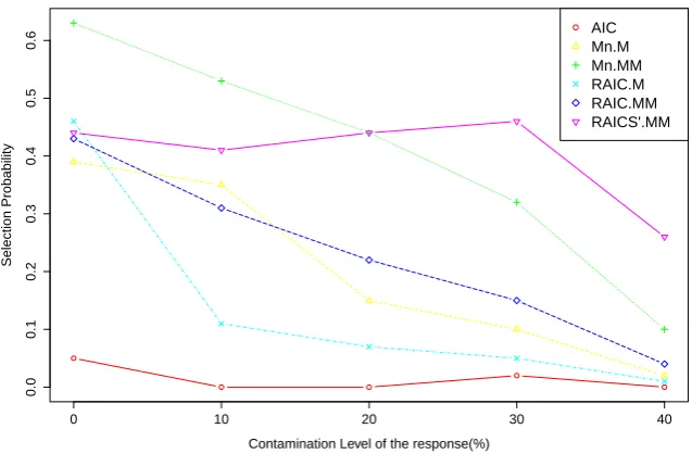
proportion of correct models than the classical AIC in the presence of outliers in the response. However, then these two criteria break down when the contam-ination level reaches 30%, as a consequence of the low breakdown point of the M-estimators. This fact is also shown in Figure 2.1. Conversely, the fourth and sixth columns suggest that when the contamination level is high, the robust model selection criteria based on MM-estimation (M n.M M and RAIC.M M) generally outperform both the classicalAIC and their counterparts based on M-estimation.

0.0

0.2

0.4

0.6

0.8

Contamination Level of the response(%)

Selection Probability

0 10 20 30 40

AIC Mn.M Mn.MM RAIC.M RAIC.MM RAICS'.MM

Figure 2.1: Selection probabilities of various model selection criteria for p= 6

(41)

Table 2.2: Bias of the robust scale estimators for the full model when p= 6

ε n=50 n=1000

% M M AD.M M M M AD.M M M M AD.M M M M AD.M M

0 -0.08 -0.10 -0.07 -0.10 0.00 0.00 0.00 0.00

5 -0.00 -0.01 0.03 -0.04 0.06 0.06 0.06 0.06

10 0.11 0.09 0.15 0.06 0.16 0.14 0.15 0.14

20 0.79 0.54 0.40 0.28 0.52 0.40 0.38 0.39

30 3.35 2.04 1.15 1.38 3.88 0.97 0.73 0.84

40 5.26 3.64 2.83 3.67 5.95 2.10 1.54 2.30

MM-estimator is at 50%. This could be explained by the bias of the robust estimation of scale as discussed in Martin et al. (1993), who argued that the maximal asymptotic bias is substantial for large ε even for the MAD, the scale estimator that we proposed for our robust model selection criteria based on loss function. We also generated 100 samples to find the average bias of the following scale estimators under our simulation setting: scale estimator from M-estimation, MAD of the residuals from M-regression, scale estimator from MM-estimation (S-estimation), and MAD of the residuals from MM-regression. Table 2.2 suggests that when the contamination level goes up, the bias of MAD increases and be-comes quite significant whenεreaches 30% forM AD.M and 40% forM AD.M M. Further, compared with the large sample case (n=1000), the bias of these scale estimators is more notable in the small sample case (n=50) that we used in our simulation setting. The loss function in the above criteria may behave less effectively when the MAD is highly biased. Therefore, these robust model selec-tion criteria do not perform as well as we expect when the contaminaselec-tion level increases. Additionally, M¨uller and Welsh (2005) also recommend using their model selection criterion only ifσ is estimated to have a small expected bias.

(42)

Impor-tantly, it is worth noting that for both of M-type and MM-type scale-based criteria the one with trace term adjusted significantly performs better than the original one suggested by Tharmaratnam and Claeskens (2013) considering various pro-portions of outliers.

1 2 3 4 5 6 7

12

16

20

24

M−estimation

Number of parameters

V

alue of penalty ter

m

1 2 3 4 5 6 7

8

10

12

14

MM−estimation

Number of parameters

V

alue of penalty ter

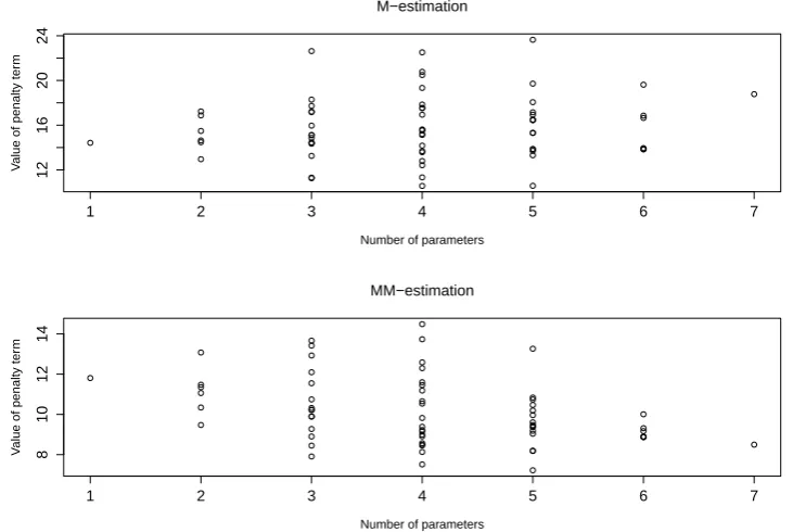
[image:42.595.88.454.203.448.2]

m

Figure 2.2: Penalty terms inRAICS.M andRAICS.M M for each possible model when p= 6, n = 50 and ε= 20%

(43)

informa-2.4. SIMULATION RESULTS 27

tion matrices, incorporating the covariance term of the covariatesxixTi . However, in Ronchetti’s computation method, the penalty term is evaluated by 2E_E[_[ψ_ψ20_]]p, in

which the expected covariance term of the covariates has already been cancelled out in the estimation procedure and the penalty term is linearly related to the number of variables in the model. Therefore, the adjusted penalty term turns out to be much more stable and it leads to a better performance ofRAIC_S0.M M

thanRAICS.M M. Though Tharmaratnam and Claeskens (2013) stated that the effect of the outliers on the penalty element of robust selection criteria based on scale estimators was seen to be non-influential, the finding under our simulation setting shows a significant improvement in the adjusted penalty term for selection probabilities. Because of the poor performance of RAICS.M and RAICS.M M, we exclude them from comparison for the rest of the simulation studies and only account forRAIC_S0.M M as a model selection criterion based on a scale estimator. Another remarkable finding is that the robust model selection criterion based on the MM-type scale-based estimator selects a higher proportion of true models as the contamination level increases up to 40 %, compared with those criteria based on the loss function. This is explained in Claeskens and Tharmaratnam (2011). When the contamination level is low (0% or 10%), the overfit model obtains a smaller scale estimate than true models on average. In such cases, the model selection criteria based on scale estimate will often select an overfit model, as a small scale estimate is preferable since we are minimizing the criteria values. However, when the contamination level goes up to 20% or 30%, the true model results in a smaller scale estimate on average than the overfit or wrong fit models. Hence, the model selection criteria based on scale estimates will more often tend to select the true model.

(44)

includ-Table 2.3: Selection probabilities for p= 6 with x-outliers

ε% AIC M n.M M n.M M RAIC.M RAIC.M M RAIC0_S.M M

0 0.05 0.39 0.63 0.46 0.43 0.44

10 0.00 0.35 0.53 0.11 0.31 0.41

20 0.00 0.15 0.44 0.07 0.22 0.44

30 0.02 0.10 0.32 0.05 0.15 0.46

40 0.00 0.02 0.10 0.01 0.04 0.26

ing M n.M M and RAIC.M M. Although the criteria based on loss function tend to perform quite well when the proportion of outliers is below 20%, the scale-based model selection criteria are preferable when the contamination level is high. Therefore, we are further inspired to choose the appropriate robust model selection criteria depending on the proportion of outliers.

0.0

0.1

0.2

0.3

0.4

0.5

0.6

0 10 20 30 40

[image:44.595.112.431.388.597.2]

Figure 2.3: Selection probabilities of various model selection criteria for p = 6 with x-outliers

(45)

Table 2.4: Selection probabilities for p= 10

ε% AIC M n.M M n.M M RAIC.M RAIC.M M RAICS.M M RAICS0.M M

0 0.31 0.25 0.46 0.30 0.27 0.02 0.09

10 0.04 0.38 0.42 0.35 0.28 0.06 0.10

20 0.00 0.30 0.47 0.13 0.31 0.09 0.32

30 0.00 0.04 0.18 0.01 0.12 0.01 0.36

40 0.00 0.00 0.06 0.00 0.00 0.06 0.20

Table 2.5: Selection probabilities for p= 10 with x-outliers

ε% AIC M n.M M n.M M RAIC.M RAIC.M M RAIC_S0.M M

0 0.00 0.28 0.40 0.11 0.22 0.10

10 0.00 0.16 0.37 0.09 0.24 0.12

20 0.00 0.05 0.27 0.01 0.09 0.23

30 0.00 0.03 0.07 0.00 0.03 0.15

40 0.00 0.00 0.01 0.00 0.00 0.14

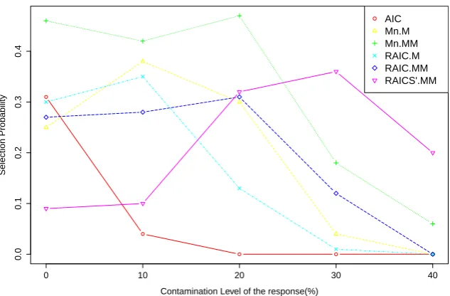
in the presence of x-outliers, the model selection criteria based on MM-estimation generally outperform those based on M-estimation even when the contamination level of is low. This is also shown in Figure 2.3 as the selection probabilities of the MM-type criteria reside above those of the M-type criteria. This strongly indicates the usefulness of the model selection criteria based on MM-estimation in the presence of both x- and y-outliers.

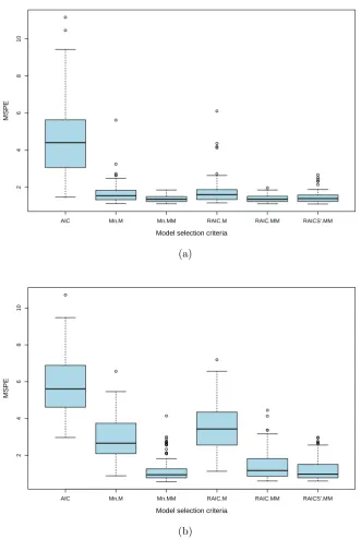
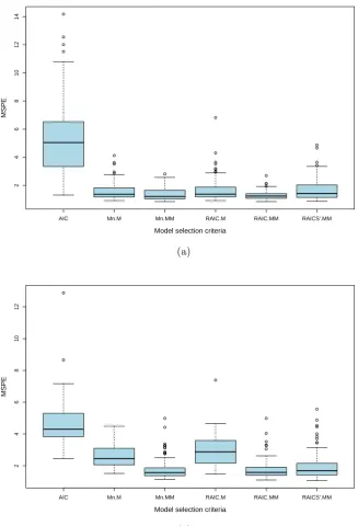
Figure 2.4 presents the mean squared predication errors forp= 6 and= 10% with and without x-outliers. From the prediction point of view, we still see very strong evidence that the robust model selection criteria outperform non-robust traditional AIC in the presence of outliers. In the presence of both x- and y-outliers, those based on MM-estimation achieve substantially lower MSPEs and significantly outperform those based on M-estimation.

We further investigate the case of p = 10. The detailed simulation results of p = 10 and n = 50 with and without outliers in the covariates are shown in Tables 2.4 and 2.5, respectively.

(46)

2

4

6

8

10

Model selection criteria

MSPE

(a)

2

4

6

8

10

MSPE

[image:46.595.106.438.152.647.2]

(b)

Figure 2.4: Mean squared predication errors for p= 6 and = 10%, (a) without x-outliers, (b) with x-outliers

(47)

0.0

0.1

0.2

0.3

0.4

0 10 20 30 40

[image:47.595.156.473.146.354.2]

Figure 2.5: Selection probabilities of various model selection criteria for p= 10

0.0

0.1

0.2

0.3

0.4

0 10 20 30 40

[image:47.595.156.474.462.670.2]

(48)

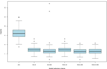
2

4

6

8

10

12

14

MSPE

(a)

2

4

6

8

10

12

MSPE

[image:48.595.108.436.155.636.2]

(b)

Figure 2.7: Mean squared predication errors for p = 10, (a) without x-outliers, (b) with x-outliers

(49)

2.5. REAL DATA EXAMPLE 33

smaller in the case of p = 10, compared with the case of p = 6. This could be expected as the selection difficulty increases when the number of variables included in the model goes up. Figures 2.5 and 2.6 suggest that similar to the case of p = 6, the criteria based on MM-estimation outperform those based on M-estimation in the presence of x-outliers or a high proportion of y-outliers. Moreover, as shown in Table 2.4 it is worth noting that the relative discrepancy of selection probabilities between RAIC_S0.M M and RAICS.M M is much larger in the case of p= 10 than in the case ofp= 6. This further indicates that when the number of variables in the model increases the original criteria as suggested by Tharmaratnam and Claeskens (2013) perform more poorly as a result of the increasing variability in the covariance term of the covariatesxixTi . Therefore, we could further conclude that the adjustment to the penalty term of the scale-based criteria improves its performance on selection probability.

From the prediction point of view, it is quite obvious that those based on MM-estimation still substantially outperform those based on M-estimation, as illustrated in Figure 2.7.

2.5 Real data example

We now apply these robust model selection criteria to analyze the well-known Boston housing data (available athttp://lib.stat.cmu.edu/datasets/boston). The data contain the following 14 variables: crim (per capita crime rate by town), zn (proportion of residential land zoned for lots over 25,000 sq.ft), indus (propor-tion of nonretail business acres per town), chas (Charles River dummy variable), nox (nitrogen oxides concentration: parts per 10 million), rm (average number of rooms per dwelling), age (proportion of owner-occupied units built prior to 1940), dis (weighted mean of distances to five Boston employment centres), rad (index of accessibility to radial highways), tax (full-value property-tax rate per $10,000), ptratio (pupil-teacher ratio by town), black (1000(Bk−0.63)2), where

(50)

[image:50.595.149.401.143.263.2]

Table 2.6: Trimmed mean square prediction error (TMSPE) for Boston housing data

Method Average TMSPE SD TMSPE

AIC 9.23 0.59

M n.M 7.43 0.34

M n.M M 7.38 0.73

RAIC.M 7.43 0.34

RAIC.M M 7.28 0.31

RAICS0.M M 7.30 0.33

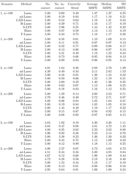
of the population in percentages), and medv (median value of owner-occupied homes in thousand dollars). There are 506 observations in the dataset. The re-sponse variable is medv. Following M¨uller and Welsh (2005), we utilized m out ofn stratified bootstrap (see M¨uller and Welsh (2005)) to generate 100 bootstrap resamples as testing samples to ensure that outliers are present in each. The comparison was then measured by the average prediction loss of these 100 testing samples (bootstrap resamples), namely, the conditional expected prediction loss. To be robust, a good model should capture the pattern of the majority of data. Therefore, we used the trimmed mean square prediction error (TMSPE), as a more appropriate measure of the prediction loss for this dataset. We truncated the largest 10 % of squared residuals and computed the TMSPE using the remain-ing 90% of the squared residuals. TMSPE is a measure of prediction accuracy for the majority of the data and is no longer dominated by extreme prediction errors. Table 2.6 and Figure 2.8 present the TMSPE for Boston housing data using different model selection criteria.

From Table 2.6, we can clearly see that the best model selected by AIC

(51)

[image:51.595.114.521.156.420.2]

2.6. CONCLUSION 35

Figure 2.8.

7

8

9

10

11

12

TMSPE

Figure 2.8: Trimmed mean square prediction error (TMSPE) for Boston housing data

2.6 Conclusion

(52)

(53)

Chapter 3 Robust Lasso Regression Using

Tukey’s Biweight Criterion

∗

3.1 Introduction

In multiple linear regression models, the ordinary least squares (OLS) estimates can give inaccurate predictions when there are a large number of predictors or multicollinearity is present. One way to improve the predictions is to reduce the number of variables in the model by model selection. Tibshirani (1996) proposed a new technique for model selection termed the “LASSO” for “Least Absolute Shrinkage and Selection Operator”, which incorporates an L1 penalty into the OLS loss function. The lasso shrinks some coefficients to exactly zero. This property of the lasso means that it provides parsimonious solutions that are easy to interpret.

Over the past decade, the lasso has become a very popular technique for simul-taneous estimation and variable selection. Many authors (Zou, 2006; Knight and Fu, 2000; Zou et al., 2007; Zhao and Yu, 2006) have investigated the properties of the lasso and developed different variants of the lasso. Zou (2006) demonstrated

∗_{The core contribution of Chapter 3 was submitted to} _{Technometrics} _{in April 2016 and}

has been accepted for publication in February 2017. This chapter was presented at the CM-Statistics Conference held in London, the UK in December 2015.

(54)

that there exist certain scenarios where the lasso is inconsistent for variable se-lection. Thus, he suggested the adaptive lasso, where adaptive weights are used for penalizing coefficients differently in the L1 penalty. The adaptive lasso enjoys the oracle property, that is, asymptotically it performs as well as if the true un-derlying model were known. Moreover, the adaptive lasso can be computed using the same efficient algorithms that are used to compute the lasso, for example, least angle regression (LARS) of Efron et al. (2004). Zou and Hastie (2005) em-phasized the inappropriateness of using the lasso as a variable selection method if a group of variables are very highly correlated. In such a situation, the lasso tends to select only one variable from the group and does not care which variable is selected. To overcome this drawback of the lasso, Zou and Hastie (2005) de-veloped the elastic net, a new regularization and variable selection method that combines anL1 and L2 penalty. The elastic net performs variable selection, con-tinuous shrinkage, and more importantly, it selects groups of strongly correlated variables. Fan and Li (2001) argued that a good penalty function should have the properties of sparsity and unbiasedness. They proposed a special non-concave penalty function named the Smoothing Clipped Absolute Deviation (SCAD) that can produce sparse solutions and unbiased estimates for large parameters.

(55)

3.1. INTRODUCTION 39

lower efficiency than OLS estimates when there are no outliers in the response. Owen (2007) and Lambert-Lacroix and Zwald (2011) preferred to replace the squared loss with Huber’s loss, a hybrid of the squared error and absolute error loss functions. Extensive simulation studies in Lambert-Lacroix and Zwald (2011) have demonstrated the superior performance of the lasso with Huber’s criterion over the traditional lasso and the LAD-Lasso.

(56)

effi-ciency when there are no outliers. Moreover, Alfons et al. (2013) do not provide any asymptotic theory for their Sparse-LTS estimator.

To be robust against outliers in both covariates and the response, the deriva-tive of the loss function needs to be redescending (Rousseeuw and Yohai, 1984; Yohai, 1987). A commonly used loss function with this property is Tukey’s bi-weight (Tukey, 1960). In this paper, we propose replacing the squared loss in the lasso with Tukey’s biweight criterion, and name the method the Tukey-lasso, to handle outliers in the response and covariates. Contemporary works based on a similar idea can be found in Smucler and Yohai (2015, 2017). In our simulation study, we show that the Tukey-lasso outperforms the adaptive lasso and other robust implementations of the lasso, particularly in the presence of outliers in both the response and the predictors.

We further propose an accelerated proximal gradient (APG) algorithm to compute the Tukey-lasso. The APG computes the lasso minimization problem and guarantees a global minimizer for a convex objective function. Although the objective function for the robust lasso with Tukey’s biweight is non-convex, the APG algorithm still achieves very reliable results (a local minimizer) when the starting value of the algorithm is carefully selected. We further demonstrate that the computation time for the Tukey-lasso through the APG algorithm is substantially lower than that of its competitors, including Rlars and Sparse-LTS.

(57)

3.2. THE LASSO-TYPE ESTIMATE 41

3.2 The lasso-type estimate

3.2.1 The traditional lasso

Consider a standard linear regression model,

yi =XiTβ+i, i= 1,2, . . . , n, (3.1) whereyiis the response variable on thei-th observation,Xi = (1, xi1, xi2, . . . , xip)T is a p+ 1 vector of covariates on the i-th observation, β = (β0, β1, β2, . . . , βp)T

is a p+ 1 vector of regression parameters, and i are independently distributed random variables with expected value 0 and variance σ2.

Although OLS estimates are unbiased, they can result in highly variable pre-dictions when no variable selection is performed. To improve prediction by shrink-ing unnecessary coefficients to 0, Tibshirani (1996) proposed to add the L1 norm of the estimates to the squared loss, leading to the lasso estimator. However, the lasso is inconsistent for variable selection, so Zou (2006) suggested the adaptive lasso in which adaptive weights are used to penalize the coefficients differently. The adaptive lasso considers the following modified lasso criterion,

argmin n X

i=1

yi−XiTβ 2

+λ

p X

j=1

b

wj|βj|, (3.2)

(58)

3.2.2 Robust lasso

It is well known that squared loss used in the traditional lasso is very sensitive to outliers. The goal of the robust lasso is to offer a more stable alternative that is not sensitive to outliers. We propose combining robust M-estimation and the adaptive lasso penalty, to obtain the generalized adaptive lasso,

argmin 2 n X

i=1

ρ

yi−XiTβ

σ

+λ

p X

j=1

b

wj|βj|. (3.3)

Whenρis the squared loss and σ= 1, (3.3) is simply the adaptive lasso (3.2). When ρ is the LAD loss, σ = 1 and the weights w_bj = 1/|βbj|, where βbj is the unpenalized LAD estimate of the jth _{coefficient, (3.3) leads to the LAD-Lasso} proposed by Wang et al. (2007). Since the squared loss in (3.2) has been replaced by the LAD criterion (L1 loss) in (3.3), the resulting estimator is expected to be more robust to outliers. The LAD-Lasso estimator produces consistent variable selection and extensive simulation studies in Wang et al. (2007) demonstrate the satisfactory finite-sample performance of the LAD-Lasso.

It is worth noting that when there are no outliers in the response, the LAD-Lasso achieves lower efficiency than the adaptive lasso. Another choice of ρ that is robust against heavy-tailed errors or outliers is Huber’s loss function. Huber et al. (1964) describes Huber’s loss function as

ρc(u) =   

u2

2 if |u| ≤c

c|u| −c2

2 if |u|> c,

(3.4)

(59)

the standard normal distribution. Therefore, when ρ is Huber’s loss function and w_bj = 1/|βb_jM|, where βb_jM denotes the unpenalized Huber estimate for the

jth _{coefficient, (3.3) leads to the robust adaptive lasso with Huber’s criterion,} discussed in Owen (2007) and Lacroix and Zwald (2011). Lambert-Lacroix and Zwald (2011) demonstrate that the lasso with Huber’s loss achieves the oracle property. More details of the estimation of β and σ are given in Lambert-Lacroix and Zwald (2011).

Although the estimates obtained from the LAD-Lasso and the lasso with Huber’s loss are resistant to outliers in the response, they are not robust against outliers in the covariates. Alfons et al. (2013) proposed Sparse-LTS by adding the L1 penalty to the least trimmed squares (LTS) criterion. The Sparse-LTS is robust with respect to high leverage points. Denote ri = yi − XiTβ, and

r2₁_n ≤ . . . ≤ r2_nn the order statistics of the squared residuals. Further define

I(r2

i ≤rhn2 ) the indicator function that equals 1 when the ith squared residual

r2_i ≤ r_hn2 . Then, when ρ= 1₂r2_iI(r_i2 ≤r2_hn), σ = 1 and the weights w_bj = 1, (3.3) reduces to the Sparse-LTS as introduced in Alfons et al. (2013). A standard choice of his h=b0.75(n+ 1)c. However, this truncation of the data may result in a loss of statistical efficiency. To overcome this loss of efficiency, Alfons et al. (2013) proposed a reweighting step to increase efficiency, Alfons et al. (2013) and our simulation study show that the Sparse-LTS performs unsatisfactorily when the data have no outliers.

3.2.3 Robust lasso with Tukey’s biweight criterion

To be robust against outliers in both covariates and responses, the derivative of the loss function needs to be redescending (Rousseeuw and Yohai, 1984; Yohai, 1987). A commonly used family of such loss functions is Tukey’s biweight,

ρd(u) =     

d2

6

1−h1− u d

2i3

if |u| ≤d

d2

6 if |u| ≥d,

(60)

where d is a tuning constant that, similar to c in Huber’s function, controls the level of robustness. Tukey’s biweight function truncates the residuals that are larger than d to the constantd2_/_{6. Therefore, small values of} _d_{imply higher}

ro-bustness while large values of dprovide higher efficiency. To achieve 95% asymp-totic efficiency at the standard normal distribution, the suggested choice of d is 4.685. We propose to replace ρ in (3.3) by Tukey’s biweight loss to deal with the outliers in both of the covariates and the response, the Tukey-lasso solves the following,

argmin 2 n X

i=1

ρd

yi−XiTβ b

σ

+λ

p X j=1

b

wj|βj|, (3.6)

whereρdis Tukey’s biweight function andbσis a robust estimate ofσ. In our study,

σ is estimated by the median absolute deviation (MAD) (Rousseeuw and Croux, 1993) of the residuals from the full model fitted by S-estimation (Rousseeuw and Yohai, 1984). Other robust scale estimates, such as S-scale estimates, are also acceptable here. Overall, we find that the performance of the Tukey-lasso is not sensitive to the choice of MAD or S-scale for estimating σ. The w_bj = 1/|βb_jM M| are weights based on the MM-estimates βb_jM M (Yohai, 1987).

Without loss of generality, we assume the true model contains the first p0

variables such that A={1,2,· · · , p0}. Write

C=  

C11 C12

C21 C22

 ,

where C11 is a p0 ×p0 positive definite matrix. To prove that the Tukey-lasso

achieves the oracle property, we make the following assumptions,

• A1: 1_nXTX→C;

• A2: max1≤i≤nkXik/

√

n→0 as n → ∞

(61)

• A4: √n(_bσn−σ) is bounded in probability.

Theorem 1. Assume conditions A1 to A4, and further suppose that λn → ∞ such that λn/

√

n → 0. Then the adaptive robust lasso estimator with Tukey’s biweight loss and preliminary scale_bσn(i.e. the Tukey-lasso) satisfies the following:

1. Asymptotic normality: √n(βb

(n)

A −βA) d

→ N(0, σ2 Eψ2d

(Eψ0_d)2C

−1

11), where Eψd2 and Eψ0_d are the expected values of ψ_d2 and ψ_d0 respectively.

2. Consistency in variable selection: limnP(An =A) = 1

Proof: The proof of Theorem 1 is provided in the Appendix A.

We use the MM-estimator to calculate the predetermined weights because the MM-estimator achieves high efficiency and is robust against both response and covariate outliers. MM-estimation is a three-stage procedure introduced by Yohai (1987). In the first stage, we compute an initial regression estimate (e.g. LMS, Rousseeuw (1984)) with a high breakdown point that is not necessarily efficient. In the second stage, an M-estimate of scale is calculated based on the initial estimator (first M). In the third stage, we compute an M-estimator of regression coefficients based on the scale estimator obtained in the second stage (second M). Briefly, the MM-estimator is computed as an M-estimator starting at a high breakdown S-estimator and with a fixed scale given by the S-estimator. For further details of MM-estimation, see Yohai (1987).

3.2.4 Robust lasso with Tukey’s biweight criterion when

p > n

(62)

The adaptive weights for the Tukey-lasso as in (3.6) are determined by un-penalized MM-estimates βb_jM M. To compute the adaptive weights when p > n, we replace the MM-estimate with MM-Ridge, as introduced in Maronna (2011). MM-Ridge is confirmed to be robust to both outliers in the covariates and the response. Further, σ_b, the robust estimate of σ, is estimated by the MAD of the residuals from the model fitted by MM-Ridge.

Simulations and real examples demonstrate that the Tukey-lasso with weights computed by MM-Ridge estimates produces reliable results when p > n. Algo-rithms for computing the Tukey-lasso are proposed in the following section. In our simulation study for both p < n and p > n, we show that the Tukey-lasso outperforms its competitors in prediction and variable selection accuracy.

3.3 Algorithms for numerical optimization

We apply an accelerated proximal gradient (APG) algorithm to compute the Tukey-lasso estimators. When the starting values of the algorithm are carefully chosen, the APG algorithm achieves very reliable results for the Tukey-lasso. Generally, the APG algorithm is very fast and also suitable for solving lasso-type problems with differentiable loss functions.

3.3.1 The traditional lasso

Consider the minimization problem,

argmin x

{F(x) := f(x) +g(x)}, (3.7)

Essays on Robust Model Selection and Model Averaging for Linear Models