promoting access to White Rose research papers
White Rose Research Online
Universities of Leeds, Sheffield and York
http://eprints.whiterose.ac.uk/
This is an author produced version of the published paper.
White Rose Research Online URL for this paper:
http://eprints.whiterose.ac.uk/5412/
Published paper
Shakhlevich, N.V. (2008) Preemptive scheduling on uniform parallel machines
with controllable job processing times. Algorithmica, 51 (4). pp. 451-473.
http://dx.doi.org/10.1007/s00453-007-9091-9
DOI 10.1007/s00453-007-9091-9
Preemptive Scheduling on Uniform Parallel Machines
with Controllable Job Processing Times
Natalia V. Shakhlevich·Vitaly A. Strusevich
Received: 28 February 2007 / Accepted: 8 March 2007 © Springer Science+Business Media, LLC 2007
Abstract In this paper, we provide a unified approach to solving preemptive
schedul-ing problems with uniform parallel machines and controllable processschedul-ing times. We demonstrate that a single criterion problem of minimizing total compression cost sub-ject to the constraint that all due dates should be met can be formulated in terms of maximizing a linear function over a generalized polymatroid. This justifies applica-bility of the greedy approach and allows us to develop fast algorithms for solving the problem with arbitrary release and due dates as well as its special case with zero re-lease dates and a common due date. For the bicriteria counterpart of the latter problem we develop an efficient algorithm that constructs the trade-off curve for minimizing the compression cost and the makespan.
Keywords Uniform parallel machine scheduling·Controllable processing times· Generalized polymatroid·Maximum flow
1 Introduction
We study the scheduling model in which the jobs of setN= {1,2, . . . , n}have to be processed on uniform parallel machinesM1, M2, . . . , Mm. For each job, its process-ing time is not given in advance but has to be chosen by the decision-maker from a given range.
N.V. Shakhlevich (
)School of Computing, University of Leeds, Leeds LS2 9JT, UK e-mail: [email protected]
V.A. Strusevich
Department of Mathematical Sciences, University of Greenwich, Old Royal Naval College, Park Row, London SE10 9LS, UK
For each jobj∈Nwe are given the interval[p
j, pj]from which the actual value
pj of the processing time is to be chosen. That selection process can be viewed either as compressing or crashing pj down topj, or decompressing pj up topj. In the former case, the value xj =pj −pj is called the compression amount of job j, while in the latter casezj=pj−pj is called the decompression amount of jobj. Compression may decrease job completion time(s) but incurs additional costαjxj, whereαj is a given unit compression cost. The total cost associated with a choice of the actual processing times is represented by the linear functionj∈Nαjxj.
The processing machines are uniform, i.e., machineMhhas speedsh, 1≤h≤m. Without loss of generality, assume that the machines are numbered in non-increasing order of their speeds, i.e.,
s1≥s2≥ · · · ≥sm. (1) A usual scheduling requirement says that a machine cannot process more than one job at a time, and a job is never processed on more than one machine at a time. Given a set of actual processing timespj,the jobs can be processed with preemption. For some schedule, denote the total time during which a jobj∈N is processed on machineMh, 1≤h≤m, byqj(h). Taking into account the speed of the machine, we call the quantityshqj(h) the processing amount of jobj on machine Mh. It follows that
pj= m
h=1
shqj(h).
Each jobj ∈N is given a release daterj, before which it is not available, and a due datedj, by which it is desirable to complete its processing. Given a schedule, let
Cjdenote the completion time of jobj, i.e., the time at which the last portion of job
j is finished on the corresponding machine. A schedule is called feasible with respect to the due dates ifCj ≤dj for all jobsj=1, . . . , n. The valueCmax=maxj∈NCj determines the maximum completion time of all jobs and is called the makespan. We exclude from further consideration the case thatn < m, since to minimize the makespan we need to processnjobs onnfastest machines.
The problem of our primal concern is to determine the values of actual processing times and find the corresponding schedule onmuniform machines so that all jobs meet their due dates and total compression cost is minimized. Extending standard notation for scheduling problems [11], we denote problems of this type byQ|rj, pj=
pj−xj, Cj≤dj, pmt n|
αjxj.Here,rj in the middle field implies that the jobs have individual release dates; this parameter is omitted if the release dates are equal. We writepj=pj−xjto indicate that the processing times are controllable andxjis the compression amount to be found. The conditionCj≤dj reflects the fact that in a feasible schedule the due dates should be respected; we writeCj≤dif the due dates are equal. The abbreviationpmt n is used to point out that preemption is allowed. Finally, in the third field we write the objective function to be minimized.
In this paper we also consider a bicriteria problem Q|pj = pj − xj,
pmt n|(Cmax, K), where K denotes a compression cost function, namely
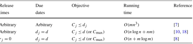
Table 1 Time complexity of the algorithms with fixed processing times
Release Due Objective Running Reference
times dates time
Arbitrary Arbitrary Cj≤dj O(mn3) [7]
Arbitrary dj=d Cj≤d(orCmax) O(nlogn+nm) [10,18]
rj=0 dj=d Cj≤d(orCmax) O(n+mlogm) [8]
defined by the break-points of the so-called efficiency frontier; see [23] for definitions and a state-of-the-art survey of multicriteria scheduling. Recall that a scheduleSis called Pareto optimal if there exists no scheduleSsuch thatCmax(S)≤Cmax(S) andK(S)≤K(S), where at least one of these relations holds as a strict inequality.
Scheduling problems with controllable processing times have received consider-able attention, see, e.g., surveys [12,16]. The study of these problems is motivated by their numerous applications to various areas. Below we discuss only computing-related applications and refer to [20] for applications of scheduling with controllable processing times to manufacturing and operations management.
In real-time systems, a common goal is to schedule processors so that all computa-tion is completed by specified deadlines because missing a deadline causes a system failure. However, meeting all timing requirements may not be possible for heavily loaded systems. In this case, some computations are performed partially, produc-ing less precise results. For example, in computproduc-ing systems that support imprecise computations, an iterative program or an image processing algorithm can often be logically decomposed. In our notation, a task with processing requirementpj can be split into a mandatory part which takesp
jtime, and an optional part that may take up topj−p
j time. To produce a result of acceptable quality, the mandatory part must be completed in full, while an optional part improves the accuracy of the solution. If instead of an ideal computation time pj a task is executed forpj =pj −xj time, then computation is imprecise andxjcorresponds to the error of computation. In this application, total compression costαjxj is the total weighted error. See [12,13,
21,22].
A similar situation occurs in computer systems that collect data from sensing de-vices where the jobs can be completed partially in order to meet their deadlines, while incomplete jobs result in information loss (see [4], Sect. 5.4.2). Decision-making in this setting is based on finding the trade-off curve between the time required to com-plete all jobs and the value of lost information.
If the processing times are fixed, the known results on finding a due date fea-sible preemptive schedule and/or minimizing the makespan on muniform parallel machines are given in Table1.
If the processing times are controllable, problem Q|rj, pj −xj, Cj ≤ dj,
pmt n|αjxj as a model of imprecise computation is studied by Błažewicz and Finke [3] and Leung [12] and shown to be solvable in O(m2n4logmn+ m2n3log2mn)andO(m2n4logmn)time, respectively.
Nowicki and Zdrzalka [17] study problem Q|pj −xj, Cj ≤d, pmt n|
O(nlogn+nm)time, but it is not clear whether their algorithm can be extended to solve the bicriteria problem in polynomial time. They also give a pseudopolynomial-time approximation scheme for finding the efficient frontier for the bicriteria problem
Q|pj−xj, pmt n|(Cmax, K).
If the machines are identical, i.e., have equal speeds, then the following two single criterion problems are studied for controllable processing times: P|pj −xj, Cj ≤
d, pmt n|αjxjandP|rj, pj−xj, pmt n, Cj≤rj+d|
αjxj. The first problem reduces to the continuous linear knapsack problem [9,20] and thus can be solved in
O(n) time while the second one reduces to linear programming [15]. The fastest algorithm for the bicriteria problemP|pj−xj, pmt n|(Cmax, K)requiresO(nlogn) time [20].
This paper is ideologically close to our previous work [20] in which several prob-lems with controllable processing times have been reduced to optimizing a linear objective function over a special polyhedron, known as a polymatroid. In this paper, for more general scheduling problems we use a more general combinatorial struc-ture of a generalized polymatroid, see Sect.2for relevant definitions. Here we only mention that the main advantage in using polymatroids is that we may simplify jus-tification of the greedy approach to solving the corresponding scheduling problems, and eventually design simpler and faster algorithms than those known earlier.
The remainder of the paper is organized as follows. Section2 reduces problem
Q|rj, pj−xj, Cj≤dj, pmt n|
αjxj to maximizing a linear function over a gen-eralized polymatroid which allows us to solve the problem inO(mn4)time by net-work flow techniques, faster than the earlier approaches [3,12]. Section3addresses problemQ|pj−xj, Cj≤d, pmt n|
αjxj with equal release dates and a common due date. Using a polymatroidal representation we arrive at anO(nlogn+nm)-time algorithm. Compared with the algorithm by Nowicki and Zdrzalka, the justification, description and analysis of our algorithm is much easier and more natural than that in [17]. The bicriteria problem Q|pj−xj, pmt n|(Cmax, K)is studied in Sect. 4. Again, the polymatroidal approach leads to an efficient and natural way of generating the break-points of the efficient frontier, thereby yielding the first polynomial-time algorithm for the bicriteria problem.
2 Arbitrary Release Times and Due Dates: Generalized Polymatroid
Consider the single criterion problem Q|rj, pj −xj, Cj ≤ dj, pmt n|
αjxj in which the jobs have arbitrary release times and due dates. Suppose that there are
q≤2ndistinct values
t1< t2<· · ·< tq
amongrjanddj,j=1, . . . , n. These values divide the time line intoq−1 intervals
Define
Sh= h
f=1
sf,
the sum of the speeds of hfastest machines, 1≤h≤m.Taking into consideration the speed of each machine, notice that in an intervalIi total processing that could be done on machineM1iss1i, on machineM2iss2i, and so on.
Given actual valuespj of the processing times of the jobs, consider the problem of finding a feasible schedule in which each jobj completes by its due datedj. For a subsetA⊆N of jobs and an arbitrary intervalIi, letAi⊆Abe the set of all jobs inAthat are available in intervalIi. If|Ai| ≥mthen allmmachines can be used for processing of the jobs ofAi in intervalIi; otherwise, the maximum total processing of the jobs of Ai in interval Ii will be achieved if |Ai| fastest machines are used. Thus, for setAthe maximum processing that can be performed in an intervalIi can be written as
ϕi(A)=iShi, (2)
wherehi=min{m,|Ai|}.
Let 2N be a set of all subsets of the jobs fromN. As proved by Martel (see The-orem 2.4.2 in [14]), a feasible schedule with job processing timespj,j=1, . . . , n, exists if and only if the following conditions hold for each subsetA∈2N of jobs:
j∈A
pj≤ϕ(A),
where
ϕ(A)=
0, ifA= ∅,
q−1
i=1ϕi(A) , otherwise.
(3)
If job processing times are controllable, then the values pj are not known in advance, but are the decision variables. It is clear that the larger actual val-ues pj are, the smaller the total compression cost
αjxj is. Therefore, problem
Q|rj, pj−xj, Cj≤dj, pmt n|
αjxj reduces to the following linear program:
max αjpj (4)
subject to the constraints
j∈A
pj≤ϕ(A), for allA∈2N,
p
j≤pj≤pj, 1≤j≤n.
(5)
Definition 1 A set-functionϕ:2N→Ris called submodular if the inequality
ϕ(A∪B)+ϕ(A∩B)≤ϕ(A)+ϕ(B)
holds for allA, B from 2N.
It is also known (see, e.g., [19], p. 767) thatϕ(A)is submodular if and only if the condition
ϕ (A∪ {j, k})−ϕ (A∪ {k})≤ϕ (A∪ {j})−ϕ (A) (6) holds for eachA⊆Nand distinctj andkfromN\A.
Lemma 1 Set-functionϕi(A)of the form (2) is submodular.
Proof We use the equivalent characterization of a submodular function (6). Recall that Ai ⊆A is the subset of jobs from Athat are available in interval Ii, so that
ϕi(A)=ϕi(Ai).
If jobj is not available in intervalIi, then
ϕi(A∪ {j, k})−ϕi(A∪ {k})=ϕi(Ai∪ {j, k})−ϕi(Ai∪ {k})
=ϕi(Ai∪ {k})−ϕi(Ai∪ {k})=0,
ϕi(A∪ {j})−ϕi(A)=ϕi(Ai∪ {j})−ϕi(Ai)=ϕi(Ai)−ϕi(Ai)=0, so that (6) holds.
Similarly, if jobkis not available in intervalIi, then we derive
ϕi(A∪ {j, k})−ϕi(A∪ {k})=ϕi(Ai∪ {j})−ϕi(Ai)=ϕi(A∪ {j})−ϕi(A), as required.
Thus, in the remainder of this proof both jobsj andkare available inIi. Denote
a= |Ai|.
Ifa≤m−2, then
ϕi(Ai∪ {j, k})−ϕi(Ai∪ {k})=iSa+2−iSa+1=isa+2≤isa+1
=iSa+1−iSa=ϕi(Ai∪ {j})−ϕi(Ai).
Ifa=m−1, then
ϕi(Ai∪ {j, k})−ϕi(Ai∪ {k})=iSm−iSm=0≤ism
=iSm−iSm−1=ϕi(Ai∪ {j})−ϕi(Ai).
Finally, ifa≥mthen
ϕi(Ai∪ {j, k})−ϕi(Ai∪ {k})=iSm−iSm=0
=iSm−iSm=ϕi(Ai∪ {j})−ϕi(Ai).
It is easy to check that each set-functionϕiof the form (2) is monotone increasing, i.e.,ϕi(A)≥ϕi(B)for all setsA⊇B. It follows that functionϕ(A)of the form (3) is submodular increasing as the sum of submodular increasing functions.
Definition 2 (Frank and Tardos [6], p. 495) A polyhedron
Pϕ=
p=(p1, p2, . . . , pn),p≥0,
j∈A
pj≤ϕ(A)for eachA∈2N
is called a polymatroid associated with ϕ if function ϕ(A) is a submodular, non-negative, monotone increasing and finite.
Thus, since function ϕ of the form (3) only takes non-negative finite values, it follows thatPϕ is a polymatroid.
Here we refrain from giving the definition of the generalized polymatroid (org -polymatroid); the reader is referred to [6], p. 501, or to [19], p. 845. For our purposes it suffices to mention that:
• a polymatroid is ag-polymatroid, see [19], p. 845;
• an intersection of a g-polymatroid with a box B = {p∈Rn,p≤p≤p} is a g -polymatroid, see [6], p. 507, and [19], p. 845;
• maximizing a linear function over ag-polymatroid can be done by a greedy algo-rithm, see [6], p. 524.
Thus, the constraints (5) define ag-polymatroid, and the problem of maximizing function (4) over it can be solved by the following algorithm.
Algorithm GrA
Step 1. If necessary, renumber the jobs so that
α1≥α2≥ · · · ≥αn. (7)
Step 2. Define pk:=pk, k=1, . . . , n.
Step 3. FOR k=1 to n do
Step 4. For job k, choose the decompression amount zk
as large as possible so that (p1, . . . , pn)∈Pϕ for
pk=pk+zk.
END FOR
For problemQ|rj, pj −xj, Cj≤dj, pmt n|
αjxj Algorithm GrA can be im-plemented in the following way. Starting with fully compressed processing times
pj =pj,j =1, . . . , n,the first task is to find an amount of processing of each job
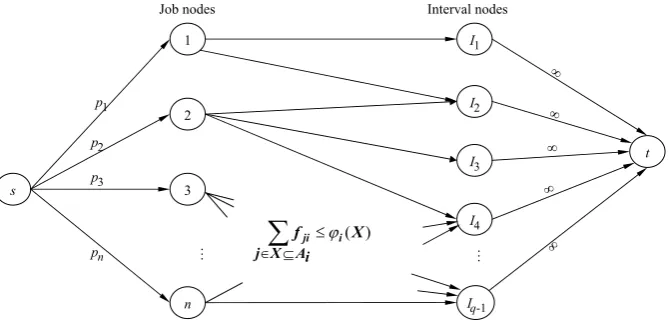
Fig. 1 Polymatroidal network by Martel
There are several ways of performing the first task. We can find the maximum polymatroidal flow of the total valuej∈Np
jin the corresponding Martel’s network (see Fig. 1); the running time of Martel’s algorithm isO(m2n4+n5)[14]. There is a more computationally efficient way of performing this task which relies on an
O(mn3)-time algorithm by Federgruen and Groenvelt [7] of solving the (ordinary) maximum flow problem in a special network (see Fig. 2).
Martel’s network containsnjob nodes connected with the source by the arcs of capacitiespj,j =1, . . . , n, andq−1 interval nodes connected with the sink by the arcs of infinite capacities. The job nodes are connected directly to the interval nodes: if jobj is available in intervalIi, then the corresponding job node and the interval node are connected by an arc with capacityS1i. Unlike the traditional maximum flow models, in the polymatroidal network additional constraints are introduced to define upper bounds on the cumulative capacities of the sets of arcs: ifXiis a (sub)set of arcs entering interval nodeIi, then the total flow on the arcs of setXi cannot be larger thanϕi(Xi), whereϕi is defined by (2). Iffj iis a flow on the arc from job nodej to interval nodeIi, then the valuefj i can be viewed as the total amount of processing of jobj in intervalIi in a feasible schedule.
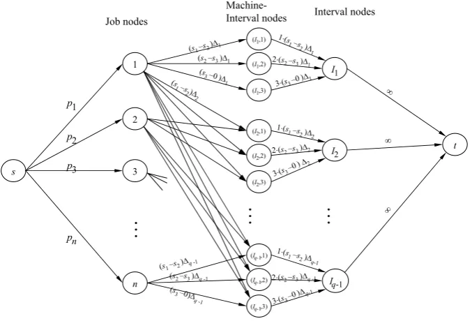
Compared with Martel’s network, in the Federgruen-Groenvelt network additional intermediate machine-interval nodes are introduced in-between the job nodes and the interval nodes. If jobj can be processed in intervalIi, then job nodej is connected withmmachine-interval nodes(Ii,1),(Ii,2) , . . . , (Ii, m)by the arcs with capaci-ties(s1−s2) i,(s2−s3) i, . . . , (sm−0) i, respectively. These machine-interval nodes in their turn are connected to the interval nodeIi by the arcs with capacities 1·(s1−s2) i, 2·(s2−s3) i, . . . ,m·(sm−0) i. Similar to Martel’s network, the total flowfj iin the Federgruen-Groenvelt network from a job nodej to an interval
Ii defines the amount of processing of jobj in intervalIi.
Fig. 2 Network flow model by Federgruen & Groenvelt
First, update the network by introducing for each arc from the source to each job nodej a lower and upper bounds on the arc capacity, both equal top
j,j ∈N. In a typical iteration (see Step 4) take the next jobk and make an upper bound on the capacity of the arc entering job nodekequal topk. Find the maximum flow in the obtained network. Letpkbe the flow value on that arc. For further iterations, set both lower and upper bounds on the arc capacity topk. Acceptpkas the actual processing time of jobk. Take the next unconsidered job with the largest compression cost, and so on.
In our implementation of Step 4 we select the Federgruen-Groenvelt model since for the networks we consider here, finding an ordinary maximum flow can be done in
O(mn3)time [2,7], faster than finding a polymatroidal maximum flow.
Recall that the process of finding the (ordinary) maximum flow with lower bounds consists of two stages: (i) finding a feasible flow and (ii) optimizing the flow; see [1]. In our case, the flow found in one iteration is feasible for the problem to be solved in the next iteration. The optimization stage deals with the so-called residual arc capacities and in our case still requiresO(mn3)time.
Since Step 4 is repeated n times, we deduce that the overall running time of our implementation of Algorithm GrA applied to problem Q|rj, pj −xj, Cj ≤
dj, pmt n|
αjxj does not exceedO
mn4.
Recall that problemQ|rj, pj−xj, Cj ≤dj, pmt n|
O(m2n4logmn), respectively, and are explicitly presented only for the case that
p
j=0,j∈N.
3 Equal Release Times and Due Dates: Single Criterion
In this section we address the simplest version of problem Q|rj, pj −xj, Cj ≤
dj, pmt n|
αjxj in which all jobs are simultaneously available at time zero, i.e.,
rj =0, and they have to be completed by a common due date d. We give an effi-cient implementation of Algorithm GrA that solves this single criterion problem in
O (nlogn+nm)time.
We adapt conditions (5) from Sect.2. Comparing problemsQ|rj, pj−xj, Cj≤
dj, pmt n|
αjxj andQ|pj−xj, Cj ≤d, pmt n|
αjxj, notice that in the latter problem all scheduling is done in a single interval I1=[0, d]. Thus, we deduce that problemQ|pj−xj, Cj ≤d, pmt n|
αjxj reduces to maximizing the linear function (4) over ag-polymatroid determined by the constraints (5) with set-function
ϕ(A)defined for anyA∈2N as
ϕ(A)=
0, ifA= ∅, dSh, otherwise,
where
h=min{m,|A|}.
Consider Step 4 of Algorithm GrA that finds the maximum decompression amount for jobk. A straightforward implementation of this step may require checking expo-nentially many inequalities from (5) that define the polymatroid. For a more efficient implementation of Step 4, determine a permutationλ=(λ(1), λ(2), . . . , λ(n))of jobs such that
pλ(1)≥pλ(2)≥ · · · ≥pλ(n), (8) breaking ties so that the jobs with equal current processing times are sequenced in non-increasing order of their compression costs. Define
Ph(λ)= h
i=1
pλ(i), h=1, . . . , m−1;
Pn= n
j=1
pj.
(9)
It is known (see, e.g., [5]) that a schedule with the makespand exists if and only if
(i) for eachh,1≤h≤m−1,hlongest jobs can be processed onhfastest machines, and
so that
Ph(λ)≤dSh, h=1, . . . , m−1,
Pn≤dSm. (10)
Clearly, it is sufficient to consider the latterminequalities together withn box-inequalities of the form
p
j≤pj≤pj, j=1, . . . , n (11) when finding the maximum decompression of jobk. In what follows, we describe an efficient implementation of Algorithm GrA based onm+n constraints (10–11) instead of an exponential number of constraints (5).
We start with fully crashed jobs withpj=pj,j∈N. Letπ be the current per-mutation of jobs, and in the beginning of the algorithm π=λ, whereλis defined by (8). During the process of decompression, the jobs will change their relative order with respect to the current processing times. Due to (9) it suffices to keep track of the firstm−1 positions of the current permutationπ of jobs. Throughout the process, we maintain the following structure of that permutation.
Definition 3 Given the current valuespj of the processing times, permutationπ of jobs is called the main permutation if
(i) the first m−1 positions of π are occupied by the longest jobs sorted in non-increasing order of pj; the jobs with equal processing times are additionally sorted in non-increasing order of their compression costsαj;
(ii) the remaining jobs are placed starting from positionm,the decompressible jobs (withpj < pj) being positioned in non-increasing order of their compression costsαj and followed by the fully uncrashed jobs (withpj =pj) taken in any order.
Determine the slacks of the constraints (10) by
τh=
dSh−Ph(π ), if 1≤h≤m−1,
dSm−Pn, ifh=m.
Consider Step 4 of Algorithm GrA in which jobk=π(u)is subject to decompres-sion. Observe that the position of jobkin that permutation cannot be larger thanm:
u≤m, (12)
since any decompressible job in positionm+1 or larger has a smaller compression cost than that of jobπ(m).
The current processing timepk can be enlarged byzk until one of the following events occurs:
Event A: jobkbecomes fully uncrashed, i.e.,pk+zk=pk;
Event B: for someh, 1≤h≤m,slackτhbecomes equal to zero;
Event C: the current value pk+zk =pπ(u)+zπ(u) becomes equal to pπ(u−1) for
If Event A takes place andu=m, then in order to maintain the properties ofπ
as the main permutation job k is moved to the last position; otherwise, if u < m, job k remains the u-th largest job and retains its position in the main permuta-tion.
If Event B happens for h=m, then in the corresponding schedule all machines are permanently busy in the time interval [0, d],so that no further decompression is possible without violating the deadlined.
If Event B takes place for h≤m−1, then in the corresponding schedule h
longest jobs and only those are processed by h fastest machines, so that no fur-ther decompression of jobsπ(1), . . . , π(h)is possible without violating the dead-lined.
Notice that decompression of job k=π(u), u≤m, does not affect the values
Ph(π )and the corresponding slacksτhforh≤u−1. Therefore, the largest possible decompressionzk such that either Event A or Event B occurs is given by
zk=min
pk−pk, τmin ,
whereτmin=minu≤h≤m{τh}.
In the case of Event C, the processing time of jobk takes the valuepπ(u−1) and that job still requires further decompressing in later iterations. In order to maintain the main permutationπwhile jobkis being decompressed, this job is swapped with jobπ(u−1). If there are more than one job with the processing timepπ(u−1), jobk is successively swapped with the jobs in earlier positions until it appears in front of all the jobs of this length.
We now give implementation details of Step 4 of Algorithm GrA for finding the optimal decompression amountzk of jobkin positionπ(u)in the current main per-mutationπ. It is assumed that we enter this step having found the valuesPn,τm,and
Ph(π ),τhforh=1, . . . , m−1.
Implementation of Step 4 of Algorithm GrA
(decompression of job k=π(u), u≤m)
Find τmin=minu≤h≤m{τh}.
WHILE pk< pk and τmin>0 DO
Compute zk=min
pk−pk, τmin, pπ(u−1)−pk .
Increase pk by zk.
Case A: pk=pk. If u=m, move job k to position π(n);
otherwise no further actions required.
Case B: zk=τmin. Set τmin:=0; no further actions
Case C: pk=pπ(u−1). j=1, τmin:=τmin−zk
WHILE pk=pπ(u−j ) DO
swap job k=π(u) with
job π(u−j ) τmin:=min
τu−j, τmin
j :=j+1
END WHILE u:=u−j+1
END WHILE
Update the values Pn, τm, Ph(π ) and τh for h=1, . . . , m−1
taking into account total decompression of job k.
Initial sorting of the machines in accordance with (1) and the jobs in accordance with (7) and (8) requiresO(nlogn)time. For the sorted jobs and machines, all sums
Pn, τm, Ph(π )andτh, 1≤h≤m−1, can be calculated inO(n)time.
In Step 4, for each job each of Events A or B may happen at most once. Due to (12), Event C occurs no more thanmtimes. Thus, the total running time of Algo-rithm GrA isO(nlogn+nm). Finding the corresponding optimal schedule requires
O(n+mlogm)time, see [8].
Example Consider the following instance of problem Q|pj − xj, Cj ≤ d,
pmt n|αjxj. There arem=3 machines with the speedss1=5,s2=3,s3=1. The due date isd =10. The processing times ofn=4 jobs and their compression costs are given in the table:
j p
j pj αj 1 2 30 8 2 10 10 1 3 50 50 1
4 1 1 1
Observe that the jobs are numbered so that (7) holds.
In accordance with Algorithm GrA, we start with fully compressed jobs with
pj =pj, 1≤j ≤4, and the main permutation π =(3,2,1,4). We enter Step 4 of Algorithm GrA having found
P1(π )=50; P2(π )=50+10=60; P4=50+10+2+1=63;
τ1=5×10−50=0;
τ2=(5+3)×10−(50+10)=20;
τ3=(5+3+1)×10−(50+10+2+1)=27.
becomes equal to 10 and we swap jobs 2 and 1 in permutationπso thatπ becomes
(3,1,2,4)andτminbecomes min{20, 19} =19.
Job 1 is further decompressed by z1=min{30−10, 19,50−10} =19, i.e., Event B occurs. As a resultp1becomes equal 29 and τmin=0. No further decom-pression of any job is possible.
To finish Step 4, we update the values ofPh(π )andτh:
P1(π )=50; P2(π )=50+29=79; P4=50+29+10+1=90;
τ1=0;
τ2=1;
τ3=0.
4 Equal Release Times and Due Dates: Two Criteria
In this section, we develop a polynomial-time algorithm for the bicriteria prob-lem Q|pj −xj, pmt n|(Cmax,
αjxj). As a solution of problem Q|pj −xj,
pmt n|(Cmax,
αjxj), we find a sequence of all break-points of the efficient frontier
(C0, K0), (C1, K1), . . . , (Cγ, Kγ), . . . , (C , K ), whereCγ is the makespan of the corresponding schedule andKγ is the total compression cost, 0≤γ≤ . For each break-point(Cγ, Kγ)an actual scheduleσγ can be found inO(n+mlogm)time, see [8].
In order to construct the first break-point(C0, K0)we crash all jobs to their min-imum processing times, i.e., set pj=pj for allj, 1≤j ≤n. Determine the main permutationπ. Recall that inπthe firstm−1 positions are occupied by the longest jobs taken in non-increasing order of their processing times. It is known (see, e.g., [5]) that for the fixed processing timespj, j ∈N, the optimum value of the makespanC is given by
C=max
Pn/Sm, max
1≤h<m{Ph(π )/Sh}
,
wherePh(π )andPnare defined by (9). DefineC0=C.In general, in the correspond-ing schedule some jobs can be uncrashed without increascorrespond-ingC0. The optimal process-ing times pj, pj ≤pj ≤pj, that minimize the total compression cost
n
j=1αjxj, can be found inO(nlogn+nm)time by solving problemQ|pj−xj, pmt n, Cj≤
C0|αjxj with a common due dated=C0by Algorithm GrA. Denote the found schedule byσ0. The corresponding value ofK0is given bynj=1αj(pj−pj), where
pj, 1≤j≤n, are actual processing times of the jobs found by Algorithm GrA. Notice that a possible structure of scheduleσ associated with a break-point(C, K)
is such that
(I) either all machines are busy in the time interval [0, C]
(II) h fastest machines, whereh < m, processh longest jobs in the time interval [0, C], while the remaining slower machines process only fully uncrashed jobs; otherwise, the total cost can be decreased by increasing the processing time of a certain decompressible job without exceedingC.
Consider an arbitrary Pareto optimal scheduleσwith the makespanC, costKand the main permutationπ. For this schedule the inequalities
Ph(π )≤CSh, h=1, . . . , m−1,
Pn≤CSm, (13)
hold, at least one of them being the equality.
In scheduleσ, take a decompressible jobklocated in theu-th position ofπ and define a blockB(u;1, g)as a partial schedule for fully occupied machinesM1, . . . ,
Mg, where g≥u, such that in (13) the inequality forh=gholds as equality and all inequalities forh∈ {u, . . . , g−1},if any, are strict. In other words, theg-th in-equality of (13) is the first inequality no higher than theu-th inequality that holds as equality.
LetB(u;1, g)be a block in schedule σ. Ifg < m, then in blockB(u;1, g)the jobs of the set N (u;1, g)= {π(1), . . . , π(u), . . . , π(g)}are processed on the ma-chinesM1, . . . , Mg and all these machines complete simultaneously at timeC. On the other hand, if g=m then in block B(u;1, g) the jobs of set N (u;1, g)=
{π(1), . . . , π(u), . . . , π(n)} =Nare processed onM1, . . . , Mm.
In line with the greedy argument, a transition from one Pareto optimal schedule to another is done by decompressing a (partially) crashed jobk=π(u)with the largest compression cost. Suppose thatkbelongs to some blockB(u;1, g). As the processing time of job k∈N (u;1, g)grows, the structure of the corresponding schedule may change, and the situation that such a change takes place determines the next break-point of the efficient frontier. A possible structural change is associated with one of the following three events:
Event U: jobkbecomes fully uncrashed;
Event V: the processing time of jobk=π(u)becomes equal to that of the nearest
longest jobπ(u−1), so that the main permutation needs to be updated;
Event W: for blockB(u;1, g)a new blockB(u;1, g)emerges, whereu≤g< g. For blockB(u;1, g)denote
P =
Pn, ifg=m,
Pg(π ), ifg < m.
Let zbe a decompression amount of job k that is being decompressed. As the processing time pk grows by z, the makespan of the resulting schedule increases by some valueδ(z). The purpose of the next lemma is to establish the relationship between these two values.
Lemma 2 Suppose that for scheduleσjobk=π(u)is subject to decompression and
kbelongs to blockB(u;1, g). If jobkis decompressed by amountzk>0 so that the
M1, . . . , Mg are permanently busy processing the jobs of setN (u;1, g)in the time
interval [0, C+δ(zk)],where
δ(zk)=
zk
Sg
. (14)
Proof SinceB(u;1, g)is a block, then in the original schedule only the jobs of set
N (u;1, g)are processed on machinesM1, . . . , Mgso that
P =CSg.
As the processing time of jobk grows by z=zk until the earliest of three events U, V or W occurs, still in the resulting schedule only the jobs of setN (u;1, g)are processed on machinesM1, . . . , Mg:
P +zk=(C+δ(zk)) Sg,
i.e., the extra processing timezk should be redistributed over the same set of ma-chines. It follows from the above two equalities, that the makespan increases by
δ(zk)=zk/Sg.
It is straightforward to verify that the decompression amount
zkU=pk−pk leads to Event U, while the decompression amount
zVk =pπ(u−1)−pk
leads to Event V. Below we present the lemma that gives a formula forzWk leading to Event W as the earliest event.
Lemma 3 Suppose that for scheduleσjobk=π(u)is subject to decompression and
kbelongs to blockB(u;1, g). If Event W is the earliest event that occurs as a result
of decompressingkbyzWk , then
zWk = min u≤h≤g−1
P Sh−Ph(π )Sg
Sg−Sh
. (15)
Proof Consider decompression of jobkby an amountz. In accordance with (13) we have that
Ph(π )≤(C+δ(z))Sh, h=1, . . . , u−1,
Ph(π )+z≤(C+δ(z)) Sh, h=u, . . . , g−1, (16) and additionally,
P+z=(C+δ(z)) Sg.
to find out when the earliest Event W occurs we need to find the smallest increment
z=zWk such that one of the inequalities withh=g,u≤g≤g−1 in (16) becomes equality, i.e., blockB(u;1, g)emerges.
For this value ofzwe have that
Pg(π )+zWk =
C+δ(zWk )Sg.
Sinceδ(zWk )=zWk /Sgdue to Lemma2, it follows that
zWk =Sg(CSg−Pg(π )) Sg−Sg
=P Sg−Pg(π )Sg
Sg−Sg
>0.
Thus, the value of zWk can be found by taking the minimum of the values P Sh−Ph(π )Sg
Sg−Sh over allh,u≤h≤g−1, which corresponds to formula (15).
Suppose that for the original problem Q|pj −xj, pmt n|(Cmax,
αjxj) we have found a sequence of break-points (C0, K0), . . . , (Cγ−1, Kγ−1). At point
(Cγ−1, Kγ−1) we know the actual processing times equal to pj =pj +zj, the main permutation π and the corresponding scheduleσγ−1 that satisfies the condi-tions where at least one inequality (13) with C=Cγ−1 holds as the equality. We describe a transition to the next break-point(Cγ, Kγ).
For schedule σγ−1 determine a decompressible job k with the largest cost αk. Assume that job k is located in theu-th position of π. We start with considering the case that schedule σγ−1 consists of a single blockB(u;1, m) that includes all machines.
The decompression amount for job k=π(u) that leads to the earliest of the Events U, V or W is equal to
zk=min
zUk, zVk, zWk
=min
pk−pk, pπ(u−1)−pk, min u≤h≤m−1
PnSh−Ph(π )Sm
Sm−Sh
,
where the last right-hand side term follows from (15).
If jobkis decompressed byzk, we obtain the next scheduleσγ that corresponds to the break-point(Cγ, Kγ)of the efficient frontier, where
Cγ =Cγ−1+ zk Sm;
Kγ =Kγ−1−αkzk.
Consider now the situation that in scheduleσγ−1 jobk1=π(u1)to be decom-pressed belongs to blockB(u1;1, g1),g1< m. For further purposes we refer to this block asB(u1;g0+1, g1), where for completenessg0is set equal to 0. Similar to the previous case we can find the decompression amountzk1=min{z
U k1, z
V k1, z
W k1}of
increaseδ1=zk1/(Sg1−Sg0)in the makespan for the jobs of setN (u1;g0+1, g1)
processed in blockB(u1;g0+1, g1); here for completenessSg0=0.
If this decompression were performed as described, we would not obtain a Pareto optimal schedule, since further decompression is possible for one or several jobs of the set{π(g1+1), . . . , π(n)}. Thus, we look for a decompressible jobk2=π(u2) such that u2> g1 and the compression cost αk2 is the largest among all
decom-pressible jobs of setN\N (u1;g0+1, g1).Temporarily disregard blockN (u1;g0+ 1, g1), and consider the subproblem of a smaller size for processing the jobs of set
N\N (u1;g0+1, g1)on machinesMg1+1, . . . , Mm. Similar to the above, for jobu2
find blockB(u2;g1+1, g2), whereg2is the smallest index,g2≥u2, for which in (13) withC=Cγ−1the corresponding inequality holds as equality. Ifg2< m, then in this block the jobs of the setN (u2;g1+1, g2)= {π(g1+1), . . . , π(u2), . . . , π(g2)}are processed on the machinesMg1+1, . . . , Mg2 and all these machines complete
simul-taneously at timeCγ−1. On the other hand, ifg2=mthen in blockB(u2;g1+1, g2) the jobs of setN (u2;g1+1, g2)= {π(g1+1), . . . , π(u2), . . . , π(n)}are processed onMg1+1, . . . , Mm. Considering blockB(u2;g1+1, g2)in a similar way as block B(u1;g0+1, g1) we can derive the formulas for the largest possible decompres-sion amount zk2 of job k2=π(u2) that leads to the earliest Event U, V or W in
block B(u2;g1+1, g2),and the corresponding incrementδ2=zk2/(Sg2 −Sg1)of
the makespan of the jobs of set N (u2;g1+1, g2). Again, ifg2=m, there are no further actions to be taken; otherwise, we search for the next decompressible job, the corresponding block, etc.
This process of identifying the decompressible jobs continues until we find a job
ky=π(uy)to be decompressed simultaneously with all previously found jobsk=
π(u),=1, . . . , y−1. The corresponding valuegyfor blockB(uy;gy−1+1, gy) is either equal tomor less thanm. In the former case, the structure of scheduleσγ−1
is described by property (I) so that all jobs of setN (uy;gy−1+1, gy)= {π(gy−1+ 1), . . . , π(uy), . . . , π(n)}are processed on machinesMgy−1+1, . . . , Mm, while in the
latter case, the structure of scheduleσγ−1is described by property (II) so that the jobs of setN (uy;gy−1+1, gy)= {π(gy−1+1), . . . , π(uy), . . . , π(gy)}and only those are processed on machinesMgy−1+1, . . . , Mgy,and all jobs that follow jobπ(gy)in the
main permutationπare fully uncrashed.
Thus, we have decomposed the problem of finding the next breakpoint into y
subproblems Q, =1, . . . , y. In each subproblem Q we consider jobs of set
N (u;g−1+1, g)on machinesMg−1+1, . . . , Mg. For each block B(u;g−1+
1, g),1≤≤y, the largest decompression amountzkof jobk=π(u)that leads
to the earliest Event U, V or W in blockBg is equal to
zk =min
zUk
, z
V k, z
W
k (17)
=min
pk−pk, pπ(u−1)−pk, min
u≤h≤g−1
P Sh−Ph(π )Sg
Sg−Sh
,
where
P =
Pn forg=m,
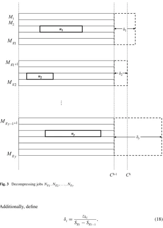
Fig. 3 Decompressing jobsNg1, Ng2, . . . , Ngy
Additionally, define
δ= zk
Sg−Sg−1
, (18)
see Fig. 3.
To guarantee that the structure of schedule σγ that defines the next break-point
(Cγ, Kγ)satisfies one of the properties (I) or (II), we need to find the largest possible value ofδ, so thatCγ =Cγ−1+δand the earliest event U, V or W occurs in one of the blocks:
Having found incrementδin the makespan value, the processing time of each job
k=π(u)increases byzkγ−1(see Lemma2):
zγk−1
=δ
Sg−Sg−1
, 1≤≤y. (20)
Observe that the values zγk−1
are defined in such a way that no Event U, V or
W occurs if the processing times of jobs k are decompressed by less than zkγ−1,
=1, . . . , y.
Summarizing, we can formalize the transition from break-point(Cγ−1, Kγ−1)to
(Cγ, Kγ)as follows.
AlgorithmT ransit ion (Cγ−1, Kγ−1)→(Cγ, Kγ)
Given: schedule σγ−1 with makespan Cγ−1 and compression
cost Kγ−1, actual job processing times pj, j∈N,
and the main permutation π.
Initialization: set δ:= ∞, g0:=0, :=0, N:=N.
1. WHILE g< m and set Ncontains jobs that are not
fully uncrashed
1.1 :=+1;
1.2 Find a decompressible job k such that
αk=maxj∈N
αj|pj< pj .
Let k=π(u). Find block B(u;g−1+1, g).
1.3 Compute zkand δ by formulas (17) and (18),
respectively.
1.4 Update N:=N\ {π (g−1+1) , . . . , π (g)} and set y:=.
END WHILE
2. Compute δby formula (19) and determine the
decompression amounts zγk−1
in accordance with (20).
Decompress jobs k1, k2, . . . , ky by the amounts
zγk−1 1 , z
γ−1 k2 , . . . , z
γ−1
ky , respectively.
3. Set Cγ :=Cγ−1+δ, Kγ:=Kγ−1−y=1αkz
γ−1
k and update
the main permutation π.
Let us estimate the running time of a single transition(Cγ−1, Kγ−1)→(Cγ, Kγ). Since each jobkis sought for among the firstmelements of the main permutation
π and their total numbery does not exceedm, all these jobs together with the jobs
gwill be found inO(m2)time. Computingzk requires at mostO(g−g−1)time
due to (17). Sincey=1(g−g−1)≤m, it follows that Steps 1 and 2 together can be implemented inO(m2)time.
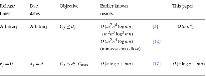
Table 2 Time complexity of the algorithms
Release Due Objective Earlier known This paper
times dates results
Arbitrary Arbitrary Cj≤dj O(m2n4logmn [3] O(mn4)
+m2n3log2mn)
O(m2n4logmn) [12] (min-cost-max-flow)
rj=0 dj=d Cj≤d;Cmax O(nlogn+mn) [17] O(nlogn+mn)
k is swapped with all the preceding jobs that have the same processing time. Even if each jobkis moved to the first position of its block, this can be achieved for job
kin no more thanmswaps. Thus, the overall time complexity of a single transition
(Cγ−1, Kγ−1)→(Cγ, Kγ)isO(m2), provided that the starting permutationπ and the partial sumsPgandSgare known.
It follows that the running time needed for solving the original bicriteria problem
Q|pj−xj, pmt n|(Cmax,αjxj)is at mostO(nlogn+ m2), where is the num-ber of break-points. To determine we count the overall number of times that each Event U, V and W may take place.
Event U occurs no more thanntimes. Event V occurs no more thannmtimes, since each time a job to be swapped is located no further than in positionmof the current permutationπ. Finally, Event W may occur no more thanmtimes in-between two consecutive Events U or V since each blockB(u;g−1+1, g)can be split in at mostg−g−1≤msub-blocks. Therefore, the number of break-points does not exceedO(nm2).
This makes the overall time complexity of finding the efficient frontier equal to
O(nlogn+nm4). Recall that for each Pareto-optimal point finding the corresponding optimal schedule requiresO(n+mlogm)time, see [8].
Observe that the approach developed by Nowicki and Zdrzalka in [17] allows finding anε-approximation of the efficient frontier in pseudopolynomialO(nm(C− C0)/ε)time, whereC andC0are the optimal makespan values if all jobs are fully uncrashed and fully crashed, respectively.
5 Conclusions
In this paper, we have extended the polymatroidal approach suggested in [20] for pre-emptive single and identical parallel machine problems with controllable parameters to a more general scheduling model with uniform parallel machines. The main out-come is establishing the link between the most general type of preemptive scheduling problems with polymatroids. This allows us to provide a unified framework for solv-ing the correspondsolv-ing problems with controllable processsolv-ing times.
leads to the design of simpler and faster algorithms than those known earlier. The results for single criterion problems are summarized in Table2.
For the bicriteria problem Q|pj −xj, pmt n|(Cmax,αjxj) of minimizing makespan and compression cost we have developed an algorithm that required
O(nlogn+nm4) time and constructs the breakpoints of the efficient frontier. It is the first algorithm that solves this bicriteria problem with uniform machines in polynomial time.
References
1. Ahuja, R.K., Magnanti, T.L., Orlin, J.B.: Network Flows: Theory, Algorithms, and Applications. Prentice-Hall, New Jersey (1993)
2. Ahuja, R.K., Orlin, J.B., Stein, C., Tarjan, R.E.: Improved algorithms for bipartite network flow. SIAM J. Comput. 23, 906–933 (1994)
3. Błažewicz, J., Finke, G.: Minimizing mean weighted execution time loss on identical and uniform processors. Inf. Process. Lett. 24, 259–263 (1987)
4. Błažewicz, J., Ecker, K.H., Pesch, E., Schmidt, G., Weglarz, J.: Scheduling Computer and Manufac-turing Processes. Springer, Berlin (2001)
5. Brucker, P.: Scheduling Algorithms, 4th edn. Springer, Berlin (2004)
6. Frank, A., Tardos, E.: Generalized polymatroids and submodular flows. Math. Program. 42, 489–563 (1988)
7. Federgruen, A., Groenvelt, H.: Preemptive scheduling of uniform machines by ordinary network flow techniques. Manag. Sci. 32, 341–349 (1986)
8. Gonzalez, T.F., Sahni, S.: Preemptive scheduling of uniform processor systems. J. ACM 25, 92–101 (1978)
9. Jansen, K., Mastrolilli, M.: Approximation schemes for parallel machine scheduling problems with controllable processing times. Comput. Oper. Res. 31, 1565–1581 (2004)
10. Labetoulle, J., Lawler, E.L., Lenstra, J.K., Rinnooy Kan, A.H.G.: Preemptive scheduling of uniform machines subject to release dates. In: Pulleyblank, H.R. (ed.) Progress in Combinatorial Optimization, pp. 245–261. Academic, New York
11. Lawler, E.L., Lenstra, J.K., Rinnooy Kan, A.H.G., Shmoys, D.B.: Sequencing and scheduling: algo-rithms and complexity. In: Graves, S.C., Rinnooy Kan, A.H.G., Zipkin, P.H. (eds.) Handbooks in Op-erations Research and Management Science, vol. 4, Logistics of Production and Inventory, pp. 445– 522. North-Holland, Amsterdam (1993)
12. Leung, T.: Minimizing total weighted error for imprecise computation tasks. In: Leung, J.Y.-T. (ed.) Handbook of Scheduling: Algorithms, Models and Performance Analysis. Computer and Information Science Series, pp. 34-1–34-16. Chapman & Hall/CRC, London (2004)
13. Leung, J.Y.-T., Yu, V.K.M., Wei, W.-D.: Minimizing the weighted number of tardy task units. Discrete Appl. Math. 51, 307–316 (1994)
14. Martel, C.: Preemptive scheduling with release times, deadlines, and due dates. J. ACM 29, 812–829 (1982)
15. Mastrolilli, M.: Notes on max flow time minimization with controllable processing times. Computing
71, 375–386 (2003)
16. Nowicki, E., Zdrzalka, S.: A survey of results for sequencing problems with controllable processing times. Discrete Appl. Math. 26, 271–287 (1990)
17. Nowicki, E., Zdrzalka, S.: A bicriterion approach to preemptive scheduling of parallel machines with controllable job processing times. Discrete Appl. Math. 63, 271–287 (1995)
18. Sahni, S., Cho, Y.: Scheduling independent tasks with due times on a uniform processor system. J. ACM 27, 550–563 (1980)
19. Schrijver, A.: Combinatorial Optimization: Polyhedra and Efficiency. Springer, New York (2003) 20. Shakhlevich, N.V., Strusevich, V.A.: Preemptive scheduling problems with controllable processing
21. Shih, W.-K., Liu, J.W.S., Chung, J.-Y.: Fast algorithms for scheduling imprecise computations. In: Proceedings of the 10th Real-time Systems Symposium, Santa-Monica, pp. 12–19 (1989)
22. Shih, W.-K., Liu, J.W.S., Chung, J.-Y.: Algorithms for scheduling imprecise computations with timing constraints. SIAM J. Comput. 20, 537–552 (1991)