A method for the measurement of hydrodynamic oil films using ultrasonic reflection

promoting access to White Rose research papers

Universities of Leeds, Sheffield and York

http://eprints.whiterose.ac.uk/

This is an author produced version of a paper published in Tribology Letters

White Rose Research Online URL for this paper:

http://eprints.whiterose.ac.uk/9189/

Published paper

Dwyer-Joyce, R.S., Harper, P. and Drinkwater, B.W. A method for the measurement of hydrodynamic oil films using ultrasonic reflection. Tribology Letters, 2004, 17(2), 337-348.

A Method for the Measurement of

Hydrodynamic Oil Films Using Ultrasonic

Reflection

R.S. Dwyer-Joycea, P. Harpera, and B.W. Drinkwaterb.

a

Department of Mechanical Engineering,

Mappin Street, University of Sheffield, Sheffield S1 3JD, UK

b

Department of Mechanical Engineering,

University Walk, University of Bristol, Bristol BS8 1TR, UK

Keywords

oil film measurement, journal bearings, hydrodynamic, fluid film bearings, ultrasound, lubrication, film thickness

Abstract

The measurement of the thickness of an oil film in a lubricated component is essential information for performance monitoring and control. In this work a new method for oil film thickness measurement, based on the reflection of ultrasound, is evaluated for use in fluid film journal bearing applications. An ultrasonic wave will be partially reflected when it strikes a thin layer between two solid media. The proportion of the wave reflected depends on the thickness of the layer and its acoustic properties. A simple quasi-static spring model shows how the reflection depends on the stiffness of the layer alone.

This method has been first evaluated using flat plates separated by a film of oil, and then used in the measurement of oil films in a hydrodynamic journal bearing. A transducer is mounted on the outside of the journal and a pulse propagated through the shell. The pulse is reflected back at the oil film and received by the same transducer. The amplitude of the reflected wave is processed in the frequency domain. The spring model is then used to determine the oil film stiffness that can be readily converted to film thickness. Whilst the reflected amplitude of the wave is dependent on the frequency component, the measured film thickness is not; this indicates that the quasi-static assumption holds.

Measurements of the lubricant film generated in a simple journal bearing have been taken over a range of loads and speeds. The results are compared with predictions from classical hydrodynamic lubrication theory. The technique has also been used to measure oil film thickness during transient loading events. The response time is rapid and film thickness variation due to step changes in load and oil feed pressure can be clearly observed.

Introduction

Current techniques for local oil film thickness measurement in bearings, by either

In this study a method which does not have these drawbacks is evaluated. An acoustic wave will propagate through a bearing shell and reflect from an oil film. The measurement of the proportion of the wave reflected can be used to determine the thickness of the oil film.

Ultrasound is routinely used for defect detection in solid bodies (Kräutkramer & Kräutkramer 1975). The principle relies on the difference in acoustic properties between the defect and surrounding material. The wave is partially reflected at a boundary between the two materials. The reflected wave is recorded and used to locate the defect. Usually these methods are carried out in the time domain (i.e. the time between the generation of the incident pulse and the reception of the reflected pulse is used to determine the defect location). However, recently frequency domain techniques have been applied to determine the integrity of adhesive layers in glued joints (Pialucha & Cawley, 1994) and other thin layers interposed between solid bodies.

In this study some of these non-destructive testing techniques have been adopted and applied to determine the thickness of oil films in real bearings without any need for intervention into, or obstruction of the oil film.

Background

Ultrasonic Reflection at an Interface

When an ultrasonic wave strikes an interface between two media, some proportion of the wave amplitude will be transmitted, whilst some is reflected. The proportion of the wave reflected, known as the reflection coefficient, R depends on the acoustic impedance mismatch between the two materials;

2 1 2 1 z z z z R  

 (1)

The acoustic impedance, z of a material is a product of its density and the speed of sound through it. Typically for a wave passing through steel and striking an oil interface, approximately 95% of the wave amplitude is reflected (R=0.95).

If a pulse of ultrasound strikes an imbedded layer of oil between two steel bodies, reflections will occur at both interfaces. In principle, the time difference between two reflected pulses could be used to measure the thickness of the oil layer. This method is commonly used in component thickness gauging, and is suitable for measuring down to around 100µm or so. Higher frequencies can be used to resolve thinner layers, but these also attenuate more

quickly. In engineering machinery the oil layers are usually much smaller than this value, and this ‘time of flight’ method is precluded.

Reflection at a Thin Layer

If the wavelength of the ultrasonic pulse is large compared to the thickness of the layer, then the layer acts as a unique reflector. The system can be treated quasi-statically and a spring model approach used. It is then the stiffness of the layer, K that determines the reflection coefficient according to (Tattersall 1973):

) ( ) ( 2 1 2 1 2 1 2 1 K z z i z z K z z i z z R      

 (2)

If the materials either side of the interface are identical z1=z2=z this reduces to:





2 1 1 z K R  

This equation can also be derived from a more general model of reflection at three layer systems (see for example Kinsler et al 2000), for the case when the film thickness is small compared with the wavelength. In most lubrication cases this holds and equation (3) can be used.

The stiffness of an interface, expressed per unit area, is given by the rate of change of pressure, p with approach of the surfaces, h:

h p K d d 

 (4)

The spring model has been used to determine the stiffness of dry rough surface contacts (Kendall & Tabor 1971, Drinkwater et al 1996), where interface consists of an array of asperity contacts. The stiffness of the interface can then be related to asperity deformation mechanics (Dwyer-Joyce et al. 2001, Krolikowski & Szczepek 1991) and contact pressure (Arakawa 1983, Quinn et al. 2002). The approach has also been used to determine the thickness and integrity of adhesive in glued joints.

If the interfacial layer is a liquid then the stiffness is obtained from its bulk modulus, B which is the pressure required to cause unit change in volume, V:

V V p B / d d 

 (5)

If the sound wave is large compared to the layer thickness, then a liquid layer is constrained to deform across it thickness only (i.e. the fluid area remains constant). Then dV/V=dh/h and:

h p h B d d 

 (6)

Combining (4), (5), and (6) gives;

h B

K (7)

The speed of sound through a liquid, c is related to the density,  and bulk modulus by:



B

c (8)

Combining (7) and (8) gives the stiffness of the layer in terms of it acoustic properties:

h c K

2



 (9)

Finally combining (2) and (9) and rearranging, gives the film thickness in terms of the reflection coefficient and properties of oil and surrounding layers.



 



For identical materials either side of the interface this reduces to:

2 2 2 1 2 R R z c h     (11)

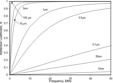
equipment operates in the frequency range 0.5 to 50 MHz. The figure shows that it is possible to use these frequencies to measure the oil films found in common hydrodynamically

lubricated machine elements.

0 0.1 0.2 0.3 0.4 0.5 0.6 0.7 0.8 0.9 1

0 10 20 30 40 50

Frequency, MHz

Reflection Coefficient,

R

10nm 50nm 0.1m

100 m 0.5m

1m 5m

10 m

Figure 1. Reflection coefficient spectra for a range of oil film thickness between steel bodies according to the spring model (equation 11).

Reflection at a Thicker Layers

0 0.2 0.4 0.6 0.8 1

0 10 20 30 40 50 60 70 80 90 100

Frequency, MHz

Reflection Coefficient

10m 100m 1m

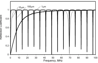
Figure 2. Reflection coefficient spectra for a range of thickness of oil film between steel bodies according to the continuum model. Within the frequency range shown, films of

100 m and 10 m show a resonance, whilst 1 m does not.

The frequency of a resonance is given by:

h cm fm

2

 (12)

where, c is the speed of sound in the lubricant layer, m is the mode number of the resonant frequency and fm is the resonant frequency (in Hz) of the mth mode. The higher resonant

frequencies correspond to thinner lubricant films. In practice the frequency is limited by the attenuation of the ultrasonic pulse in the bearing materials. So, resonances are only likely to be observed for the thicker films at higher frequencies. Typically ultrasonic testing above 60 MHz becomes difficult due to attenuation in the bearing materials. This means that if the lubricant layer is below about 10 m, the resonant frequency will be above the measurable range.

Film Stiffness or Film Resonance Methods

Film thickness measurement can thus be carried out in two ways. If the film is sufficiently thick (greater than ~15 m) then a high frequency transducer can be used to measure the film's resonant frequency. Film thickness is then obtained from equation (12). Alternatively for thin films, a low frequency transducer is used to measure the reflection coefficient and hence deduce h from equation (11).

Lower frequency transducers, coupled with the spring model approach, can be used to

measure thinner films. In this case the amplitude of the reflected signal is needed. This is then divided by the amplitude of the incident signal to get R. This method is more sensitive to noise and requires a reference signal (as described in the signal processing section of this paper). However, because a range of frequencies is being used (and not simply searching for a single resonant frequency), measurements can be recorded over a band of frequencies to give an additional check.

For the work in this paper, films in the range 0 to 30 µm have been measured using 0.5 MHz transducers. In these cases, the spring model gives adequate predictions, and a reflection coefficient method was used.

Generation of Ultrasonic Pulses and Signal Processing

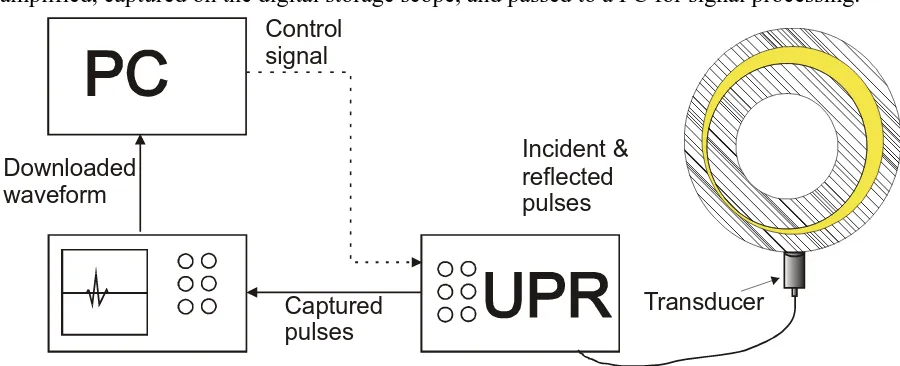
Figure 3 shows a schematic of the measurement apparatus. An ultrasonic pulser/receiver is used to generate controlled voltage pulses. These pulses are used to excite a planar piezo-electric ultrasonic transducer with a 0.5 MHz centre frequency. The transducer emits a wide band pulse and contains useful energy in the range 0.4 to 0.6 MHz. The front face of the transducer (the wear plate) is bonded directly onto the back face of the test bearing. The transducer acts as both an emitter and receiver (pulse-echo mode). The reflected pulses are amplified, captured on the digital storage scope, and passed to a PC for signal processing.

Incident & reflected pulses

Captured pulses Downloaded

waveform

Transducer Control

signal

Figure 3. Schematic diagram of the ultrasonic pulsing, acquisition, and processing apparatus.

The PC controls the UPR via the RS232 port, setting the pulsing rate, pulsing frequency and the amplification of the received signal. The PC also controls the oscilloscope for the capture of reflected signals. Thermocouples can also be interfaced with the analysis software (for monitoring of both oil film and transducer temperature).

Signal Processing

The bearing faces are then reassembled and reflected pulses from an oil film are captured, digitised, and passed to the PC. A fast Fourier transform (FFT) is performed on the pulse to give an amplitude against frequency plot. This is divided by the FFT of the reference signal to give a reflection coefficient spectra (the measured equivalent of figures 1 and 2).

Equation (11) is then used to calculate the film thickness at each measurement frequency. The reflection coefficient is a function of frequency (as shown in equation 3); lower frequencies are more readily transmitted. Clearly, the measured film thickness should be independent of the wave frequency.

The full control, acquisition, and calculation algorithms are performed by bespoke Labview software.

Tests on Static Liquid Films

A simple test rig was developed to generate a thin layer of oil between two solid steel blocks with ground and polished contact faces. One block is held stationary whilst the other is moved by means of a micrometer screw. Mineral oil (Shell Turbo T68) is placed between the block faces. A 0.5 MHz contact transducer is coupled (by means of a standard gel couplant) to the back face of one of the blocks. Pulses reflected from the oil interface were recorded for different separations of the steel blocks.

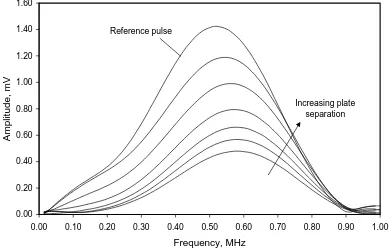
Figure 4 shows the pulse reflected from a steel-air interface (i.e. the reference pulse) and a series of spectra recorded as the plates are separated (from zero to 40 µm). As the oil film thickness is increased, the layer reduces in stiffness, and (as demonstrated by equation 3) more of the incident pulse is reflected.

0.00 0.20 0.40 0.60 0.80 1.00 1.20 1.40 1.60

0.00 0.10 0.20 0.30 0.40 0.50 0.60 0.70 0.80 0.90 1.00

Frequency, MHz

Amplitude, mV

Increasing plate separation Reference pulse

Figure 4. Fourier transforms of reflected pulses from an oil interface between two steel blocks. The amplitude of the reflected signal increases as the blocks are moved apart.

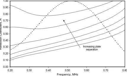
Each of the reflected pulse spectra is then divided by the reference pulse to give the reflection coefficient spectra. This is shown in Figure 5. As expected the reflection is frequency

reflection spectra. Typically any signals where the amplitude is less than 50% of the peak value (i.e. –6 dB) are discarded as being outside the bandwidth. Within the range 0.4 to 0.6 MHz the reflection coefficient is smooth and monotonically increasing with frequency.

0.00 0.10 0.20 0.30 0.40 0.50 0.60 0.70 0.80 0.90 1.00

0.20 0.30 0.40 0.50 0.60 0.70 0.80

Frequency, MHz

Reflection Coefficient,

R

Increasing plate separation

Figure 5. Reflection coefficient spectra for a series of pulses reflected back from an oil interface between two steel blocks. The reflection coefficient is frequency dependent. A

normalised amplitude spectrum is also shown to indicate the available bandwidth.

0 5 10 15 20 25 30 35 40 45 50

0.40 0.42 0.44 0.46 0.48 0.50 0.52 0.54 0.56 0.58 0.60

Frequency, MHz

Oil Film Thickness, Microns

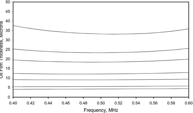
Figure 6. Film thickness determined from reflection coefficient measurements (using equation 11).

In these experiments it proved difficult to calibrate this data against a known film thickness. The spacing of the steel blocks tended to be difficult to relate to the film thickness, especially for the thinner films. Surface tension and squeeze film effects resulted in film thickness varying depending on whether the film was being increased or decreased. For this reason, no direct comparisons between ultrasonic measured film thickness and micrometer readings are given.

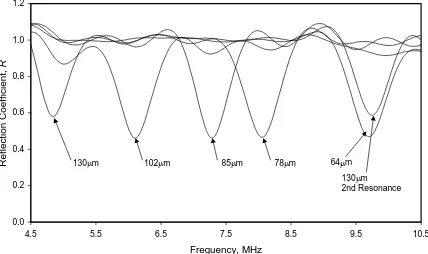
The data of figure 5 can be compared to a small section extracted from the theoretical curves of figure 1. The films are too thin to resonate at the applied frequencies. A further series of tests were carried out with a 8 MHz frequency transducer and thicker films to generate resonances. Figure 7 shows the reflection coefficient spectra for five measured films (i.e. the experimental equivalent of figure 2). The reflection coefficient spectra show clearly the appearance of minima at the resonant frequencies. The film thickness can readily be

measured from the frequency at which these minima occur using equation (12). The thickest of the oil films tested (130 µm) has both a first and second resonance within the test

0.0 0.2 0.4 0.6 0.8 1.0 1.2

4.5 5.5 6.5 7.5 8.5 9.5 10.5

Frequency, MHz

Reflection Coefficient,

R

130m 102m

130m 2nd Resonance 64m

78m 85m

Figure 7. Reflection coefficient spectra for a series of pulses reflected back from an oil interface between two steel blocks. The frequency range is such that the films resonate and

show reflection minima.

Both these film stiffness and film resonance methods can potentially be used to determine oil film thickness. As described above, the latter method is more attractive because only the frequency needs to be measured. The stiffness method requires that both amplitude and frequency are determined. However, many hydrodynamic films will be too thin to resonate at practical testing frequencies. In this work, therefore, the film stiffness method, using lower frequencies, has been used.

Journal Bearing Test Apparatus

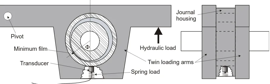
To evaluate the measurement method, a simple journal bearing was constructed. Figure 8 shows a schematic diagram. A steel journal is supported on two rolling bearings and is driven by a variable speed electric motor. A brass bush (length 37.5 mm, diameter 75 mm, and radial clearance 25 µm) is press fitted into a housing connected to a loading arm that can be

Transducer Pivot

Hydraulic load

Spring load



Minimum film

Journal housing

Twin loading arms

Figure 8. Schematic diagram of the journal bearing apparatus and transducer assembly.

A hole was through drilled in the journal hosing to give access to the bush outer surface. A 1.1 MHz planar transducer was spring loaded onto the bush as shown. A water based

ultrasonic gel is used to couple the transducer to the bush. The transducer is connected to the ultrasonic pulser-receiver and signal processing system as shown in figure 3.

The transducer in its usual position is located at the maximum load point on the bearing (i.e. at the bottom of the bearing, =0º as it is shown on the figure). The journal housing can be rotated and then fixed so that the transducer occupies a new position relative to the loading direction. Five degree graduations are marked off to accurately measure the rotation of the transducer relative to the vertical. The journal can also be rotated while the shaft is turning to measure the film thickness around part of the circumference.

A K-type thermocouple was used to measure the outlet temperature of the oil as it exited the bearing. The inlet temperature, the same as the sump temperature, was steady at 22C throughout the test. The oil temperature measurement was used to adjust the lubricant viscosity for theoretical calculations of film thickness.

Steady State Film Thickness Measurements

The same signal processing procedure used for the static film measurements was used to extract film thickness from pulses reflected from journal bearing films. This time, since the materials either side of the oil film are different (brass and steel), equation 10 is used to give film thickness.

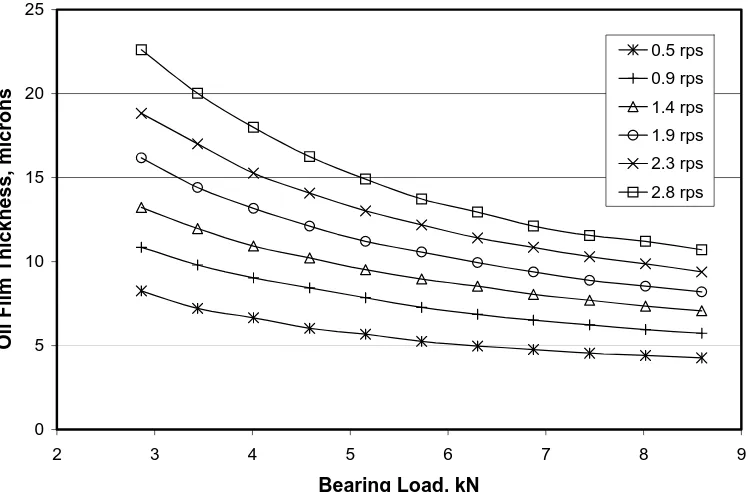
The bearing was operated under a variety of load and speed conditions and films measured using the same method as above. The results are shown in figure 9; the data is smooth and repeatable. Typically the film thickness measurements are repeatable to within 1µm.

0 5 10 15 20 25

2 3 4 5 6 7 8 9

Bearing Load, kN

Oil Film Thickness, microns

0.5 rps 0.9 rps

1.4 rps 1.9 rps 2.3 rps

2.8 rps

Figure 9. Measured lubricant film thickness (at the maximum load point) recorded for several speeds as the load is increased.

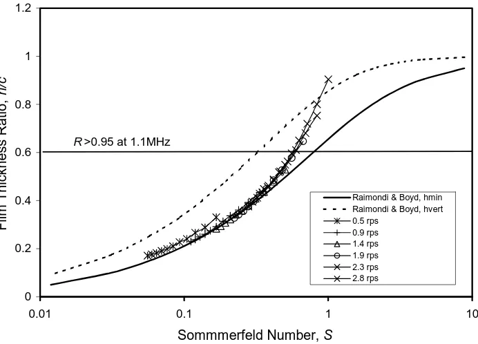
In figure 10 the data of figure 9 has been re-plotted as Sommerfeld number, S against film thickness ratio, h/c, where:

S LD

W R c

 

  

2

(13)

0 0.2 0.4 0.6 0.8 1 1.2

0.01 0.1 1 10

Sommmerfeld Number, S

Film Thickness Ratio,

h/c

Raimondi & Boyd, hmin Raimondi & Boyd, hvert 0.5 rps

0.9 rps 1.4 rps 1.9 rps 2.3 rps 2.8 rps R>0.95 at 1.1MHz

Figure 10. Film thickness measurements re-plotted on axes of Sommerfeld number against film thickness ratio. The predictions of Raimondi and Boyd (1958) are shown. The horizontal

line shows the limit of validity of the experiment (as R>0.95)

The results collapse well onto these axes; indicating essentially that the data is consistent with Reynolds’ equation.

There are several numerical solutions available for laminar iso-viscous flow in a finite dimension journal bearing. These solutions can be used to obtain both the attitude angle and bearing eccentricity ratio. The measurements reported here are recorded not at the minimum film point but rather at the maximum load point. The theoretical solution of Raimondi and Boyd [1958] has been used to predict the film thickness in this bearing both at the minimum film point and also at the maximum load point (i.e. the vertical position). These are plotted on figure 10.

There is a reasonable correlation between the theoretical and the measured film thickness values. The measured values (recorded at the vertical position) are slightly lower than expected. This may be due to the uncertainty in the viscosity of the oil (the exact oil film temperature is not known) or possibly caused by bearing misalignment.

At the higher Sommerfeld numbers the film thickness determined from the reflection coefficient departs from the theoretical trend. These thicker films are reflecting more ultrasound and the reflection coefficient is approaching unity. As R tends to unity, the film thickness measurement tends to infinity (as shown in equation 10). This means that the film tends to get over-predicted in this region. It has been found that measurements up to R=0.95 provide reliable results. The limiting film thickness where this has occurred (h=30 µm) is marked on figure 10. Strictly, once R has exceeded this value a lower frequency transducer should be used.

Transient Film Thickness Measurements

In the next experiment the transducer has been swept around part of the circumference of the bearing (over an angular arc of 0º to 90º from the loading axis) passing through the minimum thickness position. The measured film thickness is shown on figure 11. Geometrical

constraints and the location of the lubricant inlet port prevented a wider arc of measurement. The measured film thickness clearly shows a minimum value. The direction of rotation of entrainment is from left to right on the figure, as shown. Each reading is an average over three seconds.

On the entrainment side of the bearing, clear stable readings are obtained. However, over the bearing outlet region, the results fluctuate more widely. Over this region, cavitation is

occurring; the film is therefore no longer continuous but is disturbed by air pockets within the flow. The ultrasonic reflection is thus occurring at a two-phase medium; the analysis

described above will not successfully predict a film thickness. In this case the bearing speed is relatively low and so cavitation is not excessive; at higher speeds measurements in the cavitation zone may become more unstable.

If no elastic deformation of the components takes place, the geometrical shape of the gap, h between the bush and journal can be calculated from:





h (14)

where  is the eccentricity ratio given by the bearing eccentricity divided by the radial clearance (=e/c) and therefore hmin=c-e. In this case, the minimum film thickness has been

located using the measured data (i.e. the minima of the two measured and theoretical curves are coincident). As elastic deformation in this thick shelled, lightly loaded, journal is likely to be negligible, there is good agreement between the two measures of film gap (at least in the inlet region).

8 9 10 11 12 13 14 15

0 10 20 30 40 50 60 70 80 90 100

Angular Position, degrees

Oil film thickness, microns Experimental Results

Annular gap geometry

Pr

edicted minimum film location

Direction of entrainment

Figure 11. Plot of measured oil film thickness around a circular arc (measured from the loading axis). The measured data is compared against the geometrical prediction. The vertical

The work of Raimondi and Boyd (1958) can also be used to determine the attitude angle of the bearing during operation as a function of the Sommerfeld number. For the conditions of Figure 11, S=0.26, gives a value for the attitude angle of =46º. The predicted location of the minimum film is also shown on figure 11 and good agreement is observed.

Real Time Film Monitoring

Each reflected pulse is of ~3µs duration and with a repetition rate of 0.1 kHz. So, in principle, events of that duration and frequency could be recorded. However, it takes about 0.1 seconds to download a reflected pulse to the oscilloscope, and typically 20 consecutive pulses are recorded and an average used as a means of reducing incoherent noise. Each recorded data point is therefore averaging the film formed over a 2 second period. To record at a faster rate, the data would have to be stored on the scope and downloaded later for post-processing. For this work, the LabView interface was programmed to download and perform the signal processing on each data point in real time. A sample of one minute of measurements (each data point showing the film averaged over 2 seconds) is shown in figure 12.

10 10.5 11 11.5 12 12.5 13 13.5 14

0 10 20 30 40 50 60

Time, s

Oil Film Thickness, microns

7 seconds

Figure 12. Real time monitoring of oil film thickness (averaged over 2 seconds) over a one minute period. The results are also displayed as a 10 point rolling average.

There is a waviness to the recorded data (with a wavelength of ~7 seconds). This corresponds to the frequency of pulsation of the peristaltic pump used to supply oil. The oil pressure was maintained at 2 bar but the pump causes a slight fluctuation (of 0.3bar). It is interesting that the measured film fluctuation corresponds to the oil supply frequency. The solid dark line is a 10 point rolling average of the measured film; this removes the oil pressure variation effect. Step Changes in Load and Speed

0 2 4 6 8 10 12 14 16 18 20

0 100 200 300 400 500 600 700

Time, s

Oil Film Thickness, microns

38.7kN Load 700 rpm

Steady state 38.7kN 70 rpm 21.5kN Load

700 rpm Steady state

21.5kN, 350rpm

Speed ramp +70 rpm t

Load ramp +4.3kN steps

Speed ramp -70 rpm t

Figure 13. Real time monitoring of oil film thickness over a sequence of load and speed steps.

Again the scatter around the rolling average is caused by the oil feed pressure variation. The scatter is greatest at low loads (from zero to 300 seconds), as the load on the bearing

increases (from 300 to 600 seconds) the film pressure increases and then the supply pressure variation has a smaller effect on the film thickness.

Discussion

The measurement of film thickness by this means is analytically very simple. The reflection is easily related to the stiffness of the oil film using a spring model. The stiffness can, if the oil acoustic properties are known, give film thickness directly. The fact that measurements of film thickness remain constant regardless of the measuring frequency (whilst the transducer is within its bandwidth) indicate that this spring model based approach is acceptable. Whilst the concept is simple, there are a number of important practical issues that are raised here.

Curvature of the Bearing Shell

The spring model assumes a parallel flat film separated by smooth surfaces. The curvature of the journal bearing will cause some oblique reflection of the sound wave. For the relatively large journal bearing used here (D=75 mm) the curvature is large enough such that this oblique reflection is probably small. In any event, the reference trace will also have this feature and will also be proportionately reduced. So when the signal reflected back from an oil film is divided by the reference, the effect should cancel out. However, for smaller journal bearings the signal may be significantly reduced. This means that the ultrasonic wave would need to be focused.

Surface Roughness and Form

at test frequencies in the GHz region. A pocket or large dent (several millimetres) in the bearing surface could act as a separate reflector and upset the film thickness measurement. Spatial Resolution & Focusing

The transducers used in this work were all planar. The generated wave thus spreads as it travels through the bearing shell. It will therefore be reflected back from a region of film greater than the size of the piezo crystal (in this case 12.5 mm). The spatial resolution is low. To improve this, focusing transducers can be used; a spherical lens is bonded to the crystal and acts to focus the wave. In a parallel study on the measurement of elastohydrodynamic films [Dwyer-Joyce et al 2003], these transducers are used throughout. They have the

disadvantage that they need to be focused through a medium (such as water) which makes the assembly difficult.

Transducer Location

A more serious disadvantage is that measurements can only be recorded at a single place on the bearing. This means that to obtain the minimum film thickness it is necessary to use two transducers and deduce the minimum location simultaneously from equation (14), provided it can be assumed there is no elastic deformation of the housing. Alternatively an array of transducers could be used. These have recently become more wide spread in non-destructive testing applications; but have an associated cost, both financially and in terms of computing time.

Response Time

The response time of the ultrasonic approach is rapid. A pulse is typically 3 µs duration. So if the pulse can be triggered appropriately, events of that duration can be monitored. In this work the pulse repetition rate was set to 0.1 kHz. This means that, without triggering, events that occur over times greater than the spacing of two pulses (i.e. 10 ms) can be captured. The data would have to be stored and post-processed, because the download time for each pulse is of the order of 2 seconds.

It is also possible to pulse at a faster rate. The repetition rate must be such that the reflected pulse should be received before the next incident pulse is emitted. This separation will depend on the thickness of the bearing shell being looked through. For most journal bearings a pulsing rate of 20 kHz should be feasible; so events occurring at intervals of 0.05 ms can be recorded. Journal bearings do not usually operate at more than ~1000 rev/s. This pulse

repetition rate would then still allow 20 measurements during a single rotation of the bearing.

Conclusions

The oil films generated in a hydrodynamic journal bearing have been measured using a method based on the reflection of an ultrasonic wave. The proportion of the wave reflected depends on the stiffness of the oil film. A spring model approach has been used to related the reflection coefficient to the stiffness of the oil layer and hence its film thickness.

The analysis has been used on static oil films between flat steel plates. The measured film thickness is shown to be independent of the frequency of the wave used provided the transducer is within its operating bandwidth.

Measurements from a steady state hydrodynamic journal bearing have been recorded for Sommerfeld numbers in the range 0.06<S<1 and films in the range 4<h<20 µm have been recorded. The method gives repeatable results in reasonable agreement with predictions based on hydrodynamic theory.

thickness. The ultrasonic wave is reflected at the vapour pockets formed in the cavitated region. It is not possible, using this analysis, to accurately measure oil film thickness in this region.

This method has been shown to be a viable and flexible way of measuring the oil film in a lubricated journal bearing. With some practical implementation it should have applications in many other kinds of lubricated contact.

References

Arakawa, T. (1983), A study on the transmission and reflection of an ultrasonic beam at machined surfaces pressed against each other, Materials Evaluation, Vol.41, pp. 714-719. Drinkwater, B.W., Dwyer-Joyce, R.S. and Cawley, P., (1996), A study of the interaction between ultrasound and a partially contacting solid-solid interface, Proc. R. Soc. Lond. A, Vol. 452, pp. 2613-2628.

Dwyer-Joyce, R. S., Drinkwater, B. W., and Quinn, A.M., (2001), The use of ultrasound in the investigation of rough surface interfaces”, ASME J. Trib., Vol. 123, pp. 8-16.

Dwyer-Joyce, R.S., Reddyhoff, T., and Drinkwater, B. (2003), Operating limits for acoustic measurement of rolling bearing oil film thickness, submitted to Tribology Transactions. Kendall, K. and Tabor, D., (1971), An ultrasonic study of the area of contact between stationary and sliding surfaces, Proc. R. Soc. Lond. A, Vol. 323, pp. 321-340.

Kinsler, L.E., Frey, A.R., Coppens, A.B., Sanders, J.V., (2000), Fundamentals of Acoustics, Wiley, New York.

Kräutkramer, J. and Kräutkramer, H., (1975), Ultrasonic Testing of Materials, Springer-Verlag, New York.

Krolikowski, J. and J. Szczepek, (1991), Prediction of contact parameters using ultrasonic method, Wear, Vol. 148, pp. 181-195.

Pialucha, T. and Cawley, P., (1994), The detection of thin embedded layers using normal incidence ultrasound, Ultrasonics, Vol. 32, pp. 431-440.

Quinn, A.M, Drinkwater, B.W., and Dwyer-Joyce, R.S., (2002), The measurement of contact pressure in machine elements using ultrasound, Ultrasonics, Vol. 2002, pp 495-502.

Raimondi, A.A. and Boyd, J., (1958), A solution for the finite journal bearing and its application to analysis and design -I -II, -III, ASLE Trans., Vol. 1, No. 1, I- pp. 159-174, II- pp. 175-193, III- pp. 194-209.