Evaluation of the EVA Descriptor for QSAR Studies: 3. The use of a Genetic Algorithm to Search for Models with Enhanced Predictive Properties (EVA_GA)

This is a repository copy of

Evaluation of the EVA Descriptor for QSAR Studies: 3. The

use of a Genetic Algorithm to Search for Models with Enhanced Predictive Properties

(EVA_GA)

.

White Rose Research Online URL for this paper:

http://eprints.whiterose.ac.uk/175/

Article:

Turner, D.B. and Willett, P. (2000) Evaluation of the EVA Descriptor for QSAR Studies: 3.

The use of a Genetic Algorithm to Search for Models with Enhanced Predictive Properties

(EVA_GA). Journal of Computer-Aided Molecular Design, 14 (1). pp. 1-21. ISSN

1573-4951

https://doi.org/10.1023/A:1008180020974

[email protected] https://eprints.whiterose.ac.uk/

Reuse

Unless indicated otherwise, fulltext items are protected by copyright with all rights reserved. The copyright exception in section 29 of the Copyright, Designs and Patents Act 1988 allows the making of a single copy solely for the purpose of non-commercial research or private study within the limits of fair dealing. The publisher or other rights-holder may allow further reproduction and re-use of this version - refer to the White Rose Research Online record for this item. Where records identify the publisher as the copyright holder, users can verify any specific terms of use on the publisher’s website.

Takedown

If you consider content in White Rose Research Online to be in breach of UK law, please notify us by

White Rose Consortium ePrints Repository

http://eprints.whiterose.ac.uk/

This is an author produced version of a paper published in

Journal of

Computer-Aided Molecular Design

.

White Rose Repository URL for this paper:

http://eprints.whiterose.ac.uk/archive/175/

Published paper

Turner, D.B. and Willett, P. (2000) Evaluation of the EVA Descriptor for QSAR

Studies: 3. The use of a Genetic Algorithm to Search for Models with Enhanced

Predictive Properties (EVA_GA). Journal of Computer-Aided Molecular Design,

14 (1). pp. 1-21.

Evaluation of the EVA Descriptor for QSAR Studies: 3. The use of a Genetic

Algorithm to Search for Models with Enhanced Predictive Properties (EVA_GA)

David B. Turner* and Peter Willett

Krebs Institute for Biomolecular Research and Department of Information Studies,

University of Sheffield, Western Bank, Sheffield, S10 2TN, U.K.

Key words: AM1, CoMFA, GA, MM3, molecular vibration, variable modification

Summary

The EVA structural descriptor, based upon calculated fundamental molecular vibrational

frequencies, has proved to be an effective descriptor for both QSAR and database similarity

calculations. The descriptor is sensitive to 3D structure but has an advantage over

field-based 3D-QSAR methods inasmuch as structural superposition is not required. The original

technique involves a standardisation method wherein uniform Gaussians of fixed standard

deviation (σ) are used to smear out frequencies projected onto a linear scale. This smearing

function permits the overlap of proximal frequencies and thence the extraction of a fixed

dimensional descriptor regardless of the number and precise values of the frequencies. It is

proposed here that there exist optimal localised values of σ in different spectral regions; that

is, the overlap of frequencies using uniform Gaussians may, at certain points in the

spectrum, either be insufficient to pick up relationships where they exist or mix up

information to such an extent that significant correlations are obscured by noise. A genetic

algorithm is used to search for optimal localised σ values using crossvalidated PLS

regression scores as the fitness score to be optimised. The resultant models are then

validated against a previously unseen test set of compounds. The performance of EVA_GA

is compared to that of EVA and analogous CoMFA studies.

Introduction

EVA is a molecular descriptor that is derived from calculated fundamental infra-red (IR)

and Raman range vibrational frequencies [1,2,3]. The descriptor has the advantage over

popular 3D-QSAR methods such as CoMFA [4] in as much as it is invariant to rotation and

translation of the structures concerned and it is therefore not necessary to superpose

compounds in order to provide descriptors. Extensive studies [2,3] have indicated that EVA

can successfully be used to develop QSAR models for a range of different structural classes,

exhibiting various degrees of conformational freedom and with a variety of biological

endpoints. These studies also found that EVA, like field-based 3D-QSAR, can perform well

*

with heterogeneous sets of structures. In most cases the EVA models were found to be

statistically entirely comparable to those obtained using CoMFA but without the difficulties

associated with structural superposition. A detailed study with a benchmark steroid dataset

[3] indicated that EVA can provide statistically robust QSAR models when this is judged by

the scores from internal crossvalidation, random permutation tests and external test set

prediction.

This paper describes a modification to the way in which the EVA descriptor is calculated

that has been developed with a view to providing QSAR models with enhanced internal and

external predictivity. The "classical" EVA descriptor (henceforth referred to as EVA) is

derived by projecting normal mode frequencies (NMFs) onto a linear scale and then

smearing them out using Gaussian kernels such that proximal frequencies are permitted to

overlap. A fixed-dimensional standardised descriptor is then extracted for any chosen

molecule, as described in more detail below. Previously, for a given analysis, EVA has been

extracted using Gaussian kernels of fixed standard deviation (σ) across the spectrum. This is

necessary because it means that each frequency (i.e., each part of the spectrum) is equally

weighted prior to regression analysis. It has been found that the quality of the QSAR model

very often is dependent upon the chosen σ and that the best σ to use can vary substantially

[2,3]. The general approach [3] has been to generate many sets of EVA descriptors based

upon a variety of σ and, on the basis of training set crossvalidation results, select a σ

expansion term that is expected to provide an optimally predictive model for a previously

unseen test set. The effectiveness of this model-selection method has been clearly

demonstrated with a steroid dataset [3].

In the work described herein σ has been permitted to have localised values at different

regions on the linear scale. This approach should permit the determination of an optimal or

near-optimal overlap of kernels across the spectrum, where the quality of this overlap is

judged by the scores from subsequent PLS regression using the derived descriptor matrix.

The basis of this study is the postulate that there exist localised values of σ associated with

different regions of the spectrum that provide improved internal and external predictivity

relative to those obtained with any model based on a fixed σ term. At the same time there is

a requirement to search for an optimal set of these σ values and, for reasons explained

below, a genetic algorithm (GA) has been used to direct this search. PLS [5] crossvalidation

regression scores are used as the fitness function to be optimised by the GA. The proposed

technique is fundamentally different from more standard variable selection techniques [6-8]

information content (i.e., the selection of frequencies contributing to a variable) that is

altered through the adjustment of kernel overlap.

An incentive for the development of this new approach to EVA, referred to hereafter as

EVA_GA, is that there are a number of datasets with which EVA has previously not

performed well [2], either in absolute terms or relative to CoMFA – the reasons for this

under-performance are not apparent. In addition to the potential for providing improved

QSAR predictions, it may be the case that the use of localised σ improves the possibilities

for interpretation of an EVA QSAR model (i.e., back-tracking to structure).

Methods

Notation

The following is an alphabetic list of abbreviations related to PLS analyses: A − number of

PLS LVs; CV − crossvalidation; F − Fischer significance score; G − number of CV groups;

LOO − leave-one-out CV (G = M); LNO − leave-n-out CV, where n > 1; LVopt− optimum

number of latent variables (LVs); M − number of training set molecules; pr2− test set

predictive-r2; PRESS − predictive residual sum of squares; q2− LOO CV r2; r2− fitted

model r2; SE and SECV− Standard Error and CV-SE; TG − training set; X − matrix of

descriptor variables; Y − dependent variable (bioactivity etc.)

For the EVA descriptor and EVA_GA the following abbreviations are used: BFS − linear

bounded frequency scale; CONV_CRIT − difference between fitness scores of the least and

most fit members of a GA population; H − Hamming threshold; LVmax− number of LVs

evaluated by EVA_GA; MAX_CYCLES − maximum number of GA generations;

N − number of atoms in a molecule; NBINS − number of bins into which BFS is divided;

NMF − normal mode frequency; NPOP − number of GA chromosomes; R − set of r σ

values from which elements of V are selected; V − a GA chromosome; Vopt− an optimal V.

Software and Hardware

All the work described herein was carried out using a multiprocessor Silicon Graphics

Origin 200 R10000. The molecular modelling software used was Sybyl 6.3 [9]. The

software required to run the GA, to perform the EVA standardisation process and to do the

Classical EVA

The EVA descriptor [1,2] is derived from fundamental molecular vibrational frequencies of

which there are 3N-6 (or 3N-5 for a linear compound such as acetylene) for an N-atom

structure. The frequency values are projected onto a linear bounded frequency scale

covering the range 1 to 4,000 cm-1 and then smeared out, and therefore overlapped, through

the application of Gaussian kernels to each and every frequency value. Finally, the BFS is

sampled at fixed intervals of L cm-1. The value of the EVA descriptor at a point, x, on the

BFS is the sum of amplitudes of the overlapped kernels at that point:

EVA 1

2p i 1 3N 6

e (x f ) /2

x i

2 2

= =

−

∑ − −

σ

σ

where fi is the i th

normal mode frequency of the compound concerned.

This process is repeated for each dataset structure, thus providing a descriptor of fixed

dimension for all compounds. Typically a descriptor set may be derived using a σ of 10 cm-1

and an L of 5 cm-1 resulting in 800 (4,000/L) descriptor variables [1]. The number of

variables is thus very much larger than the number of compounds in a standard QSAR

dataset and the Partial least squares to Latent Structures (PLS) technique [5] has been used

to provide a robust regression analysis. The purpose of the EVA smoothing procedure is not

to simulate an experimental IR spectrum (transition dipole data is not used and, therefore, all

kernels are of fixed maximum amplitude) but rather it is to apply a density function such

that vibrations at slightly different frequencies in different compounds can be "overlapped"

and thus compared with one another. The extent of this overlap is governed by σ and the

proximity of vibrations on the BFS.

Localising σ

In classical EVA the kernels have a uniform fixed standard deviation (equal width, height

and shape) for all frequencies in all compounds while, as stated above, σ is here permitted to

have localised values in different spectral regions. The local values are to be selected so as

to improve model predictivity and, as with the selection of a suitable fixed σ value, training

set CV is used to select an optimal set of localised σ.

There are a number of ways in which the concept of a localised σ might be applied to

EVA-descriptor generation. It is possible to associate each and every NMF in each and every

compound of a dataset with its own localised σ value. Such a scheme would, however, only

be appropriate were there not to be a requirement to make external test predictions, since

including them in the optimisation procedure. In addition, the number of adjustable

parameters would be extremely large (M × (3N-6)) for typical QSAR datasets. It was,

therefore, decided to divide the BFS into NBINS bins of equal width (w), with each of

which a localised σ value is associated. The Gaussian kernel for any frequency in any

structure whose value falls within a given bin (spectral sub-region) is thus expanded using

the σ associated with that bin. NBINS (4,000/w) is thus independent of both M and the

number of NMFs (proportional to N). A potential solution is thus a vector, V, consisting of

NBINS elements:

V = { σ1, σ2, σ3, … σNBINS-2, σNBINS-1, σNBINS }

Each of the NBINS sub-regions cannot be independently evaluated because the information

content of descriptors located in adjacent bins is generally not independent: except where σ

is very small indeed, kernels centred in adjacent bins tend to overlap one another thus

adding additional signal (or noise) to the descriptors concerned. The extent of such overlap

depends upon the relative frequency values and the local σ applied. Only the main spectral

sub-regions (the fingerprint / functional group-stretching and hydrogen-stretching) are

sufficiently far apart on the BFS such that there is no overlap unless σ were to be extremely

large (Figure 1).

Without imposing constraints upon the values that local σ can assume the search space is

huge; e.g., if only integer values in the range 1 to 50 cm-1 were to be permitted then full

coverage of σ space would require a search of 50NBINS permutations. Therefore, a restriction

is placed on the values that local σ can assume and are taken from a user-defined r element

vector (R) where:

R = { σi, σii, …, σr-1, σr }

A suitable set of values for R may, for example, be {5, 10, 15, 20, 40} and a solution V has

elements taken from R. The use of a representative set of discrete values such as these is

justified since previous work has shown that for small changes in σ there tends to be little

difference in the ensuing PLS scores [2,3]. For a particular dataset, R may be selected to

reflect results obtained when using a range of fixed σ values; i.e., one may wish to bias the

solution toward previously obtained results. The total number of permutations where r = 5 is

thus 5NBINS which, where w = 40 cm-1, is equivalent to 5100 (~1070). In practice there are

substantial regions of the IR spectrum in which there tend to be no NMFs (Figure 1),

particularly outside the skeletal region (~1,500–4,000 cm-1). This feature means that, for the

62. This significantly reduces the available permutations to 562 (~1043) but nonetheless

remains a large search space. A σ value of zero has not been permitted here since this would

allow NMFs to be omitted from consideration altogether, although this may form the basis

of a variable selection procedure.

A second problem that arises with the use of localised σ values is that, without some form of

scaling, there will be variance that is related solely to the chosen σ (i.e., kernel maximum

amplitude differences) rather than to differences in frequency value location on the BFS.

Therefore, all kernels are scaled to a maximum amplitude of unity prior to determining the

local EVA descriptor values. This means that the kernels differ only in terms of their width,

and to a lesser extent, shape (Figure 2) rather than height, shape and width.

Searching for an Optimal Solution (Vopt) EVA_GA

As stated previously the number of possible solutions to be explored is immense and all

possible permutations of the elements of V cannot be evaluated systematically. Therefore, a

technique is required that permits a sampling of the search space in as thorough a manner as

possible without the requirement to cover that space in its entirety. Genetic algorithms

[10,11] provide an obvious and convenient means to approach the stated problem. GAs are

now a well-established stochastic technique for performing directed random searches of a

problem space and have been widely applied to drug design and chemometric problems

[12]. A wide variety of alternative formulations are available the selection of which are to

some extent arbitrary; details of the chosen methods are given below while Figure 3 is a

generalised overall schema for EVA_GA.

A. Chromosome encoding. In the current context a chromosome conveniently consists of

the vector, V, described above. In order to ensure the diversity of the initial population a

Hamming threshold (H) was applied such that at the outset each chromosome was permitted

to have a maximum of H genes of identical value to those of any other chromosome. The

minimum possible value of H depends upon NPOP, NBINS and the number of possible

different values associated with each bin (r).

B. Chromosome fitness evaluation. The chromosome fitness function is the q2 score from

PLS CV based upon an EVA descriptor set derived using V; the higher the q2 score the

greater the chromosome fitness. Both LOO and LNO CV have been implemented the

advantages and disadvantages of these two approaches are discussed below. The SAMPLS

algorithm [13] provides a highly efficient implementation of PLS-1 and, for univariate Y

SAMPLS is based upon reduction of the X block data to an M-by-M covariance matrix of

all the pair wise "distances" between each of M molecular descriptor vectors which is then

used to fit all PLS LVs independent of the original number of variables. SAMPLS was

custom-written so as to provide a very efficient implementation and full integration with the

GA and EVA descriptor code; for example, with M = 21 and 1000 variables LOO CV using

five LVs required only ~0.01 seconds.

C. Reproduction. The reproductive stage involves three steps; viz. parent selection,

crossover and mutation. Parents are selected using the roulette wheel method whereby

parents are selected in a probabilistic manner in which those with a higher fitness are more

likely to be selected than those with lower fitness. However, an élitist model [15] also was

implemented in which the best member of the current parent population is forced to be in

next generation. Both single and double crossover points are permitted, the selection of

which is done at random as are the points at which crossover takes place. Mutation is

permitted at random points on a randomly selected chromosome − a chromosome may be

selected for mutation (or crossover) more than once − and, while the σ at the mutated point

is selected at random from R, the new value is forced to be different from the current value.

Child population duplicates are mutated in the same way. The probability, Pm, of mutation is

set to 0.05 (although this can be altered by a user) this is somewhat higher than a typical

value of 0.01 and was chosen to encourage exploration of the large search space. The

probability, Pc, of crossover is also user-definable but was fixed at 0.85 herein.

D. Evaluation of ultimate GA solution(s). The optimal solution(s) provided by the GA is

(are) evaluated against a previously unseen set of compounds (the test set) where such is

available. This enables one to test for over-fit to the training set and must be considered a

crucial model validation procedure where, as here, a large number of adjustable parameters

(σ) are involved. Training set random permutation tests also are applied to all Vopt and

estimates made that the observed q2 and r2 scores could be chance effects; 1,000

permutations of the activity data were made in every case.

E. PLS model selection strategies. The selection of model-dimensionality (LVopt) and thus

the fitness score (q2) of a particular chromosome during evolution of the GA requires careful

consideration. Scoring on the basis of the first q2 maximum (keyword: MAX_Q2) provides

the most obvious method. However, in the interests of efficiency it is desirable to extract as

few LVs as possible while at the same time model parsimony is, in general terms,

can be favoured by using, for example, a formula for calculating SECV that penalises

additional LVs [16]:

(

)

SE PRESS / (M A 1)

CV

1/2

= − −

Thus, models can be extracted on the basis of the first SECV-minimum (keyword:

SECV_MIN). Alternatively, or additionally, a 5% rule (keyword: 5%_RULE) may be

applied [16] wherein an additional LV is permitted only where it raises q2 by ≥ 0.05 units. In

general, but not always where M is small, the latter method is at least as parsimonious as the

SECV_MIN approach. However, the purpose of the GA is to search for better solutions, the

quality of which are judged by the q2 scores. A "better" solution can be seen as any vector,

V, that provides a higher q2 than obtained previously. An q2 improvement may be very

small, and may require an additional LV in comparison to other models with slightly smaller

q2 but may provide an intermediary model in the progress toward a significantly better

solution. It is, therefore, arguable as to whether MAX_Q2, SECV_MIN or the 5%_RULE

should be the model selection criterion and various comparative tests are made using

otherwise identical EVA_GA runs.

An upper bound to the value of LVopt is that it should not exceed M/4 since the use of a ratio

greater than this results in increased probability of chance correlation [17]. Finally, it is not

acceptable to make predictions of the biological activity of structures to greater precision

than the error in (reproducibility of) the original measurements. This factor has been directly

addressed for the steroids [3] while the relevant information is not available for the

melatonin compounds.

F. Default EVA_GA parameters. The following set of default GA parameters are defined:

CONV_CRIT = 0.05 (i.e. there is no significant difference between the fitness scores of the

most and least fit population members); MAX_CYCLES = 100; NBINS = 100 (i.e.,

w = 40 cm-1); NPOP = 100; PLS_MODEL_SELECTION = 5%_RULE. Crossvalidation can

be LOO or LNO; unless otherwise stated, in the latter case G = 7 and CV is repeated 50

times and mean values reported for q2 and SECV. Parameters such as R and LVmax are set

according to the dataset involved and can be based upon examination of a range of results

with EVA.

Datasets

The performance of EVA_GA was evaluated using datasets for which external test sets were

available and consist of a benchmark steroid dataset [4,18,19] and a set of melatonin

EVA_GA QSAR model since the large number of adjustable parameters (NBINS) means a

priori that there is great potential for training set overfit.

Steroids. The steroid set consists of 21 TG and 10 test set compounds (Table 1), originally

investigated (in terms of 3D-QSAR analysis) by Cramer et al. [4]. This dataset has been

described in detail previously together with both CoMFA and EVA analyses [3] and is not

described further here; the activity data are measured corticosteroid-binding globulin

affinities expressed as log [K]. The PLS results with EVA were good and it is of interest to

determine whether or not EVA_GA can enhance this in any way. Whilst this dataset has

been widely used as a benchmark for novel QSAR methods [18] it completely lacks any sort

of experimental design; seven of the ten test set compounds have structural features not

explicit in the training set. With this in mind statistical experimental design techniques

[21,22] have been applied to these structures as described below. It is legitimate to make

quite precise predictions of the steroid binding affinities − a lower bound to the SE of ~0.08

(equivalent to r2> 0.995) has previously been estimated [2].

Melatonin. The melatonin receptor ligands (Table 2 and Figure 4) consist of a TG of 44

structures and a test set of 9 structures taken from a 3D-QSAR investigation by Sicsic et al.

[20]. This TG (analysis "J" in Ref. 20) provided the best CoMFA model selected from a

range of different TGs having up to 48 compounds and should thus provide a stringent test

of the relative performance of EVA/EVA_GA. The TG ("T" name prefix in Table 2)

consists of five classes of structure, including 9 indole, 21 naphthalene, 2 tricyclic, 2

tetraline and 10 benzene-based compounds. The test set ("Z" name prefix) consists of 9

compounds, 7 of which belong to the benzene, naphthalene or tricyclic classes and which to

some extent reproduce structural features present in the TG. However, there are no explicit

TG examples of the m-ethoxy substituents of the test compounds Z55 and Z56, one of the

test set compounds is a quinolinic structure (Z49) and compound (Z50) is structurally

related to one of the naphthalene compounds. There are, therefore, four test set compounds

which a priori might be expected to (but need not necessarily) provide predictive problems

for a QSAR model.

Both the TG and test set compounds exhibit binding affinities (pKi) covering five orders of

magnitude for chicken brain melatonin receptors (Table 2). The 44 TG compounds

thoroughly and regularly span activity space (Figure 5). However, two of the test set

compounds (Z49 and Z56) have lower activity than any of the 44 TG structures while only

one of the TG compounds (T04) is less active than Z54. Not only is Z56 the least active

compound overall but there is a gap of ~0.54 pKi units between it and the least active TG

once again, therefore, an expectation that there are likely to be predictive difficulties

particularly with compound Z56 and, possibly, Z49. In the original CoMFA study [20]

structure T47 has lower activity than Z56 but was excluded from the best CoMFA analysis

since it was considered an outlier, a not unreasonable finding given that its pKi is ~0.6 units

lower than that of T04.

Calculation of Normal Mode Frequencies (EVA)

Semiempirical. The steroid dataset was treated using the AM1 Hamiltonian of MOPAC 6.0

[23] with the parameters described previously [3]. The conformations used for the CoMFA

analyses were adopted as the starting points for the MOPAC geometry optimisation of all

structures. None of the 31 structures had imaginary ("negative") normal mode frequencies,

indicating that the optimized geometries were at or very close to a stationary point

MM3 Molecular Mechanics. The melatonin ligands were geometry minimised using

MM3(94) [24] molecular mechanics. As with the steroids, CoMFA conformations [20] were

used as the starting points for the MM3 runs. The MM3 FULL_MATRIX option is required

for a FORCE calculation to be done; all other MM3 parameters were left at their default

values. Eleven of the structures had one imaginary NMF but the most negative of these was

only -28.9 cm-1. The calculations are in any case unreliable from -50 cm-1 to 50 cm-1 so

NMFs within this range are not significant; imaginary NMFs are excluded from

consideration when generating the EVA descriptor.

CoMFA Analyses

For both datasets CoMFA analyses were performed so as to provide benchmark values

against which to judge the performance of EVA/EVA_GA. The steroid CoMFA analysis

has been described in some detail previously [3]; the structures and conformations are those

of Wagener et al. [19] and were aligned using an RMS fit of the 3, 5, 6, 13, 14 and 17

skeletal carbon atoms (Figure 6) with deoxycortisol (H11) as a template. For the melatonin

ligands the superposed conformations were obtained directly from the original authors [20].

Most of the melatonin ligands have a highly flexible ethylamido side-chain (Figure 4) so the

CoMFA alignments are based upon atom-based RMS fitting to the restrained tricyclic

compounds (T33 and T34) using the alignment centres defined in that Figure.

CoMFA was undertaken using a 1 Å grid-spacing rather than the default 2 Å. There is

considerable evidence to suggest that results with the latter spacing are likely to be

unreliable [8] and, therefore, the CVR2-GRS (Crossvalidated-r2-Guided Region Selection)

method [8] − an unsophisticated domain-based variable selection procedure − was applied to

grid-spacing through reorientation tests, in which all compounds are reoriented as an aggregate

rigid body within the bounding CoMFA 3D grid. This was done systematically, at fixed

intervals of either 1° and 10° through 360° in each plane separately and in various

combinations, and training and test set modelling and prediction performed for each

orientation; this provides a means of estimating the stability and true statistical performance

of the CoMFA PLS models. Evaluations such as this incorporating test set predictions have

not been previously published.

Aside from the grid resolution all other CoMFA parameters were kept at the Sybyl default

values. MOPAC 6.0 AM1 [23] charges were used for the steroid analysis while Sybyl [9]

Gasteiger and Marsili charges were utilised with the melatonin receptor ligands per the

original publication [20]. As with the EVA analyses LOO or LNO (steroids only) CV was

used with a maximum of M/4 LVs depending on the dataset size. Analyses were done using

steric and electrostatic fields combined and were performed for unscaled and blockscaled

data. Sybyl PLS was used for CoMFA regression analysis and models were selected on the

basis of the SECV_MIN rule noted above.

Results and Discussion

Steroid Dataset

CoMFA and EVA. As stated above the chosen steroid dataset previously has been

investigated in some detail using both EVA and CoMFA [3] and only brief comments will

be made here. With EVA the best models with fixed σ were obtained where σ = 3/4 cm-1

(Table 3). These models had a q2 of 0.80 (two LVs) and a pr2 of 0.69 or 0.76 (excluding an

outlier (M31) with a fluorine substituent not explicit in the TG). Test set predictions for σ

values other than 3/4 cm-1 rapidly become very poor (Figure 7) so there is a quite distinct,

limited range of optimal fixed σ for this dataset. The melatonin dataset on the other hand

has a much broader (contiguous) band of σ values over which pr2 scores are relatively stable

(see below). CoMFA modelling with this steroid dataset (Table 3) provides a very high q2

score of 0.87 (two LVs) and an equally high test set pr2 (0.84) where the fluorine outlier is

excluded. However, the CoMFA model is extremely sensitive to M31 and, when it is

included in the test set, the pr2 score drops to 0.45. It has been suggested that this difference

between CoMFA and EVA reflects the different information content of the vibrational and

field-based descriptors. It is therefore of interest to determine whether or not optimisation of

the EVA model using EVA_GA alters the sensitivity of the method to M31. It should also

aggregate reorientation [3] the test pr2 scores show the greatest variation, ranging from

0.42 to 0.48 (all compounds) and 0.81 to 0.86 (M31 excluded).

EVA_GA To start with the default GA parameters noted above were used together with R

= {1, 2, 3, 4, 5} and LVmax = 2 both chosen according to EVA results (Figure 7, Table 3).

However, a wide variety of alternatives parameters were investigated also (Tables 4−7). The

most obvious feature of most of the results obtained is that it is possible to enhance q2 by up

to 0.08 units (LOO CV) and 0.06 units (LNO CV) relative to the best EVA model (Table 3).

The best predictive results are obtained where two or more LVs are available to EVA_GA

and in general, but not exclusively, two LVs are optimal for both TG and test set

predictions. Where two or more LVs are available test set pr2 scores (0.70-0.75) are virtually

identical or slightly smaller than that obtained with EVA. Again, provided at least two LVs

are available, EVA_GA is not sensitive to the PLS model selection criteria and there is

nothing to be gained from setting MAX_CYCLES > 100 (Table 5) although, where

MAX_CYCLES = 50 the results over five runs of the GA show considerable variation. In

addition EVA_GA is not sensitive to the alternative values of NBINS that were investigated

(Table 6).

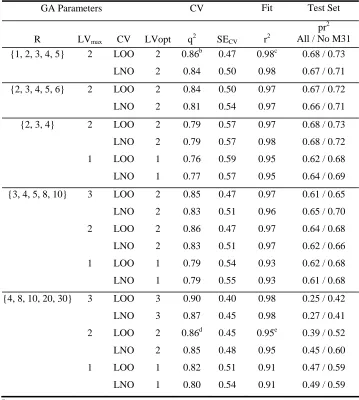
EVA_GA appears to be most sensitive to the choice of R set values (Table 7). For example,

if relatively large σ such as 20 and 30 cm-1 are made available to the GA then, whether one,

two or three LVs are used, LOO q2 is enhanced (to 0.82. 0.86 and 0.90 respectively) while

pr2 scores are very poor where either M31 is included (0.47, 0.39 and 0.25) or excluded

(0.59, 0.52 and 0.42); LNO-based searches provide only slightly better results in some

cases. This is a similar finding to that with EVA where pr2 scores (and TG CV scores) are

poorer where σ is not very close to 4 cm-1 (Figure 4). Examination of the Vopt solutions for

each of the five GA runs indicates that large σ are incorporated into the solutions when

made available. Random permutation tests applied to two sets of results where R = {1, 2, 3,

4, 5} and {4, 8, 10, 20, 30} and where LVmax is two (Table 7 footnotes) indicate that (for

LOO q2) in the latter case the estimated probability of chance correlation (p) is 0.021 for

LV1 (i.e., greater than 1%) and 0.0005 for LV2 (mean p over 5 GA runs) while in the

former case p is 0.0007 or 0.0006 for one or two LVs respectively. Thus, it seems that the

possibility for chance correlation is greatly increased where large σ are used. Where the

fitted-r2 is considered, in all cases p < 2.7 × 10-13. Thus, even in the absence of the poor test

set predictions where R = {4, 8, 10, 20, 30}, the models based on the R set with smaller σ

As noted above the steroid dataset lacks any sort of experimental design, statistical or

otherwise, and in view of this the dataset as a whole was re-examined using PCA and PLS.

It is acknowledged, however, that implicit in EVA_GA are changes to the descriptor space

and that experimental design can be properly applied only where descriptor space is

constant. However, we proceed on the assumption that some sort of design consideration is

better than none at all. As an initial step PLS CV was applied to all 31 structures (σ = 4 cm

-1

) giving a q2 of 0.75 (two LVs) against which the scores from subsequent designed models

can be compared; note that a total of 21.9% of the X block (i.e., EVA descriptor) variance is

explained by these two LVs. A PCA (no scaling) was then applied to the 31-compound X

matrix. However, 19 PCs are required to explain 90% of the variance in X∗ with the first

seven PCs explaining (cumulatively) 15.1%, 25.4%, 34.5%, 41.8%, 47.5 %, 52.8% and

57.8% respectively − additional PCs explain < 5% further variance. The number of design

points (compounds) required for a two-level factorial design (FD) with k variables (here,

significant PCs) is 2k and that for a fractional FD (FFD) is 2k-1 (ignoring centre-points). Thus

even where k = 7 and a two-level FFD is applied there is a requirement for a minimum of 64

compounds. This is in any case an unsatisfactory summary of the univariate variance in X

since 42.2% is left unexplained where only 7 PCs are considered. Therefore, further analysis

was done so as to eliminate compounds that might be considered outliers: this can be done

either in terms of the X space alone or in both X and Y space combined. Outliers in X space

can be identified using Hotelling's T2, a multivariate generalisation of Student's t-test, which

provides an elliptical confidence region for the data when viewed as two-dimensional score

plots. Using 0.01 as a confidence limit, and through examination of all score plot

combinations up to 7, 19 (90 % of X explained) and 30 (100 % of X explained to three d.p.)

PCs, then 0 compounds, 4 compounds (M1, L16, M27 and M31) and 10 compounds

(previous four plus: H7, L13, H19, H20, M21, M24) respectively can be considered

significant outliers. When these compounds are excluded and PCA repeated 16 or 14 PCs

respectively are required to explain 90% of the variance in the reduced descriptor blocks.

Even with a 0.05 confidence limit for T2, using which threshold 21 compounds can be

excluded, 7 PCs are required to explain 90% of the variance in X for the remaining 10

compounds; clearly too many design variables where only 10 compounds are available.

Thus, even where the chemical justification for excluding compounds is ignored, it seems to

be the case that experimental design in PC space is difficult if not impossible with these

compounds and this descriptor.

In consequence of the difficulty of performing a PCA-based design it was decided to do a

design in the PLS LV space which focuses attention upon the variance in X that is related to

∗

Y and is, therefore, a supervised or biased design. As noted above LOO CV using all 31

compounds provides LOO/LNO q2 scores of 0.75 / 0.74 (2 LVs) − an additional LV does

not improve q2 any further. Clearly, a FD with only two significant variables requires only

four data points. However, ten data points is generally considered to be the minimum

required for PLS analysis and, therefore, further compounds were selected, including

centre-points, so as to span the LV space thoroughly, giving a new TG consisting of L4, H6, H7,

L9, L13, L18, H22, H23, M26, M27 and H30 (DESIGN_A). EVA analysis (Table 8)

provided an optimal model where σ = 4 cm-1 with LOO/LNO q2 scores of 0.55 / 0.54 (one

LV) − which are somewhat less than all-compound CV − with an r2 of 0.89 and a pr2 of 0.51

(or 0.55 excluding M31). It is to be expected that CV using a sparse, designed set of

compounds give a lower q2 relative to instances where there is much redundancy.

Application of EVA_GA to DESIGN_1 (Table 8) provided enhanced q2 and r2 scores (0.71

and 0.96 respectively) while the pr2 score was, once again, not significantly altered whether

or not M31 is included in the test set.

A second design was made (DESIGN_B) but this time the three largest outliers from

all-compound CV (H22, M27, H31) were excluded entirely. With EVA this set of 28

compounds provided optimal LOO/LNO q2 scores of 0.84 / 0.83 (2 LVs) where σ = 4 cm-1.

Ten compounds were picked from an LV score plot as before (Table 8) which provided an

EVA model with LOO/LNO q2 scores of 0.69 / 0.66 (2 LVs) and a pr2 of 0.69; that is, both

predictive scores are reasonably high and their values very similar indicating that here q2 is

good indication of model predictivity. The application of EVA_GA (Table 8) provided

enhanced q2 scores (0.81 with 2 LVs) and a slightly reduced pr2 score (0.66, whether M31 is

included or not). Thus, overall it appears that there is nothing to be gained or lost in terms of

test compound predictivity through the application of EVA_GA with the various steroid

training / test sets evaluated.

Melatonin Receptor Ligands

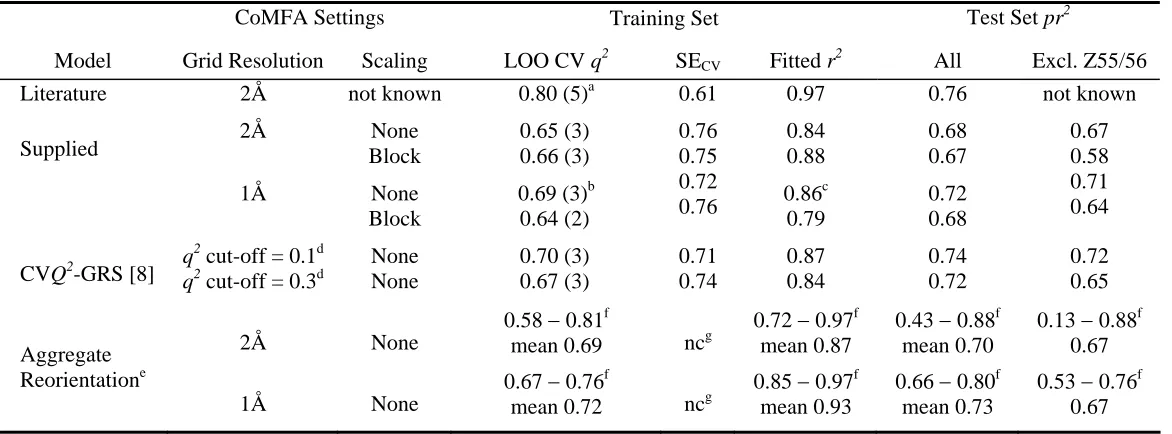
CoMFA Results. A CoMFA was performed using a set of aligned structures obtained

directly from Sicsic et al. [20]; note that for reasons discussed above dataset "J" was

selected from that paper. The results of our CoMFA are listed in Table 9 together with those

obtained by the original authors. It is apparent that our results differ somewhat from those of

Sicsic et al. despite ensuring as far as possible that the CoMFA parameters were identical.

The reason for this is most likely that, as noted above [8], a 2 Å grid resolution usually adds

a sampling error into the descriptors in as much as the results obtained depend upon the

orientation of the structures as an aggregate body relative to the 3D grid. For this reason a 1

orientation-independent results. Indeed, the mean PLS scores (q2, r2, pr2) of ~3,800 reorientations of the

aggregate using a 2 Å resolution are almost identical to the single orientation 1 Å results

(Table 9); this also applies where mean values from the same set of reorientations are

assessed at a 1 Å grid-spacing. The range of PLS scores obtained is extremely wide at 2 Å,

particularly for the test set predictions ( >0.4 units), and the scores obtained by Sicsic et al.

certainly fall within these limits. At a 1 Å resolution the PLS scores are more stable

covering ~0.1 units for q2 and r2 while pr2 scores again show the greatest variance ranging

from 0.66 to 0.80 for all nine compounds and from 0.53 to 0.76 where Z55 and Z56 are

excluded. What is more there is only a very low correlation between q2 and pr2 (r = 0.15) so

choosing a suitable orientation on the basis of CV scores provides no indication as to what

the true pr2 may be. Overall, these results indicate that a 2 Å resolution is inadequate with

this dataset and that test set scores can show significant variation even at a 1 Å resolution.

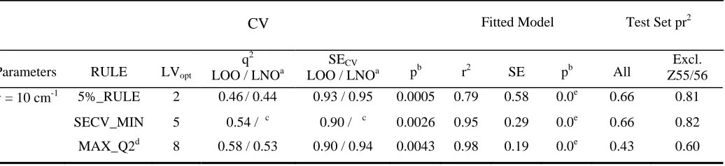
EVA Results. A large number of EVA descriptor sets derived using a range of different

fixed Gaussian σ were evaluated on the basis of training and test set statistics. It is clear

from the LOO CV results (Figure 8) that the best training set models are those where σ =

3−15 cm-1, depending upon which LVs are considered. LV1 is maximal where σ< ~4 cm-1,

while the addition of LV2 and subsequent LVs results in progressively higher peaks where

σ≈ 10 cm-1. Thus, where σ = 10 cm-1 (Table 10),if the 5%_RULE is applied q2 is 0.46 (2

LVs), while a model based on SECV_MIN has a q2 of 0.53 (5 LVs). If MAX_Q2 is the

selection criterion then q2 = 0.58 (8 LVs); this is in fact the highest observed q2 for all

models where a maximum of ten LVs are extracted. Thus, whatever criterion is used to

select LVopt, and thence the optimal σ to use, q2 is not particularly high. Test set predictions

where σ = 10 cm-1 are, on the other hand, somewhat better (Table 10) with the parsimonious

models providing the best pr2 scores of 0.66 for all nine compounds and ~0.81 (2 or 5 LVs)

if the previously noted outliers (Z55/Z56) are excluded. Overall, with this data set, and in

contrast to the steroid results, the selection of LVopt and the best fixed σ is not clear cut. In

comparison to CoMFA these EVA results are poorer, particularly where q2 is considered

while there are much smaller differences in pr2 scores. The EVA predictions are quite

sensitive to the presence of compounds Z55 and Z56 (~0.15 units difference) while this is

less the case for CoMFA − 0.06 units difference where the mean values of aggregate

reorientation at 1 Å resolution are considered (Table 9).

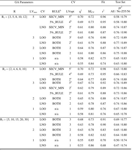
EVA_GA. As previously, an initial R set was chosen based upon σ values centred around

the optimal EVA training set σ of 10 cm-1 (Figure 8); thus, R1 = {3, 5, 8, 10, 12}. These

results also suggest that LVmax should be two or three; the larger value was chosen since this

choices of parameters are considered below. The PLS_MODEL_SELECTION method was

the 5%_RULE since this provides the most straightforward selection of LVopt from the

optimal solutions produced by the GA.

If the results where R = R1, as suggested by the EVA results, are considered (Table 11) it is

apparent that it is always the cases that solutions can be obtained with EVA_GA that have

substantially higher q2 than EVA. It is also the case that this improvement does not require

additional LVs. Indeed, the one-LV EVA_GA models have roughly the same LOO/LNO q2

(~0.58/~0.53) as the eight-LV EVA model (Table 10) and test set predictivity that is equal

to that of the optimal EVA models (pr2 = ~0.65 or ~0.80, including and excluding Z55/Z56

respectively). If further LVs are made available to the GA then it is clear that two or three

LV models provide the best test set scores (~0.75 / ~0.88) representing worthwhile

improvements over the EVA scores. Even where five LVs are made available to the GA,

LVopt is indicated to be two or three provided that the more conservative LNO CV is used

for fitness scoring during population evolution. The use of LOO CV for fitness scoring

where LVmax> 3 produces the highest q 2

scores (up to 0.70 with LVopt = 4 or 5) but the

models begin to show signs of overfit to the TG (pr2 = ~0.58 / ~0.79). If an alternative R set

is considered (R2 = {2, 4, 6, 8, 10}) the results (Table 11) are almost identical to those with

R1 as might be expected, the only substantive difference being the better pr 2

scores where

LVmax = 5. If very much larger σ are made available to the GA (R3 = {5, 10, 15, 20, 30}) q 2

scores can be enhanced to similar levels as with R1 and R2 while their is little or no

improvement in pr2 scores relative to EVA where LVmax> 1. Where only one LV is

available q2 and test set scores are poorer than when more LVs are available as was found

also with sets R1 and R2. The findings with R3 suggest that lower σ help to limit the

possibilities for TG overfit − this was even more strongly indicated with the steroid results

(Table 7). In any case the EVA results over a range of fixed σ (Figure 8) suggest that the use

of large σ would not be useful. Note that none of the models listed (Table 11) are

contraindicated by random permutation tests at any number of LVs.

Thus far the results described have been with default EVA_GA settings and a variety of R

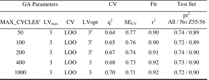
sets and LVmax. The results with alternative MAX_CYCLES (Table 12) suggest that 100

cycles is certainly adequate, where the other parameters are their default values, and there is

clearly little or nothing to be gained from using more than 100 GA iterations. Where only 50

iterations are available the mean score values (over five GA runs) are similar to those where

more runs are used but, as with the steroids, there is much greater variation in the scores

over the five runs and 100 iterations is preferred. Where alternative bin widths are

100 or 200 while poorer scores are obtained where NBINS ≥ 400 despite the improvements

to q2. However, even where NBINS = 800 (~5425 available permutations where empty bins

are excluded) and MAX_CYCLES = 1,000 (Table 13) test set predictions remain at least as

good as those with EVA (Table 10).

Conclusion

A method has been described that explores an alternative formulation of the EVA QSAR

technique (EVA_GA) incorporating the localisation of the values of the main EVA

parameter, the Gaussian kernel width (σ). A genetic algorithm has been used to explore

localised "σ space" using the scores from LOO or LNO PLS crossvalidation as the fitness to

be maximised by the GA. When applied to a benchmark steroid dataset, for which really

quite good results had already been obtained using classical EVA, the EVA_GA could

always find improved training set models but for the most part test set predictivity was

improved not at all. However, except with certain parameter choices (availability of high σ)

contraindicated by both the classical EVA results and random permutation tests, test set

predictivity was as good as that with EVA. Similar results were obtained where the training

/ test division of structures was modified using statistical experimental design criteria.

With a second relatively heterogeneous set of melatonin receptor ligands, representing five

structural classes, the results obtained were much more encouraging. Again, it was always

found that higher q2 scores (typically, up to 0.25 units better) could be obtained with

EVA_GA compared to fixed σ EVA. However, in contrast to the steroid results, test set

predictive scores were also substantially enhanced in most cases. As with the steroid set the

availability (and incorporation by EVA_GA into optimal solutions) of σ values larger than

those suggested by the EVA results leads to indications of training set overfit. Where large

numbers of latent variables are made available to EVA_GA the possibilities for overfit

increase although, with this melatonin dataset, the use of the more conservative LNO PLS

crossvalidation helps to control model dimensionality such that this avoided.

Overall, additional work is needed so as to verify that EVA_GA is an effective technique, to

attempt to generalise these findings into a set of parameters that might be expected to be

widely applicable, and to examine the obtained models in detail so as to look at what

changes are being made by EVA_GA in descriptor space. Further development of EVA_GA

might include the incorporation of some limited form of random permutation testing into the

chromosome scoring function, perhaps simply to reject a chromosome entirely if it fails to

more standard variable selection procedures in which variables may be removed from

consideration entirely; i.e., permit σ to be zero.

Acknowledgements

We thank: the Biotechnology and Biological Sciences Research Council (BBSRC) for

funding; Tripos Inc. for the provision of software; and the following for providing the

QSAR datasets:- Sames Sicsic, Université de Paris-Sud (melatonin receptor ligands) and

Johann Gasteiger, Universität Erlangen (steroids). This paper is a contribution from the

Krebs Institute for Biomolecular Research, which is a designated Biomolecular Sciences

Centre of the BBSRC.

References

1 Ferguson, A.M., Heritage, T., Pack, S.E., Phillips, L., Rogan, J. and Snaith, P.J., J. Comput.-Aided Mol. Design, 11 (1997) 143.

2 Turner, D.B., Willett, P., Ferguson, A.M. and Heritage, T., J. Comput.-Aid. Mol. Design, 11 (1997) 409.

3 Turner, D.B., Willett, P., Ferguson, A.M. and Heritage, T., J. Comput.-Aid. Mol. Design, in press.

4 Cramer, R.D., Patterson, D.E. and Bunce, J.D., J. Am. Chem. Soc. 110 (1988) 5959. 5 Wold, S., Ruhe, A., Wold, H. and Dunn III, W.J., SIAM J. Sci. Stat. Comput., 5 (1984)

735.

6 Cruciani, G. and Clementi, S., In van de Waterbeemd, H., (Ed.) Methods and Principles in Medicinal Chemistry, Vol. 3, Advanced Computer-Assisted Techniques in Drug Discovery, VCH, Weinheim, Germany, 1995, pp. 61-88.

7 Lindgren, F., Geladi, P., Rannar, S. and Wold, S. J., Chemometrics, 8 (1994) 349. 8 Cho, S.J. and Tropsha, A., J. Med. Chem., 38 (1995) 1060.

9 Tripos Associates Inc., 1699, South Hanley Road, St. Louis, MO 63144.

10 Goldberg, D.E., Genetic Algorithms in Search, Optimisation, and Machine Learning, 1995, Addison-Wesley, Reading, MA, USA.

11 Michaelewicz, Z., Genetic Algorithms + Data Structures = Evolution Programs, Second edition, 1992, Springer-Verlag, Berlin, Germany.

12 Clark, D.E. and Westhead, D.R., J. Comput.-Aided Mol. Design, 10 (1996) 337. 13 Bush, B.L. and Nachbar, Jr, R.B. J. Comput.-Aided Mol. Design, 7 (1993) 587. 14 De Jong, S., Chemometrics Intell. Lab. Syst., 18 (1993) 251.

15 De Jong, K.A., An analysis of the behaviour of a class of genetic adaptive systems, 1975. Doctoral dissertation, University of Michigan, USA.

16 Wold, S., Johansson, E. and Cocchi, M., In Kubinyi, H. (Ed.) 3D QSAR in Drug Design. ESCOM, Leiden, 1993, pp. 523-550.

17 Topliss, J.G. and Edwards, R.P., J. Med. Chem., 22 (1979) 1238.

18 Coats, E.A., In Kubinyi, H., Folkers, G. and Martin, Y.C. (Eds.) 3D QSAR in Drug Design: Recent Advances. Perspectives in Drug Discovery and Design, Vols. 12/13/14. Kluwer/ESCOM, Dordrecht, The Netherlands, 1998, pp.199-213.

20 Sicsic, S., Serraz, I., Andrieux, J., Brémont, B., Mathé-Allainmat, M., Poncet, A., Shen, S. and Langlois, M., J. Med. Chem., 40 (1997) 739.

21 Austel, V., In van de Waterbeemd, H., (Ed.) Methods and Principles in Medicinal Chemistry, Vol. 2, Chemometric Methods in Molecular Design, VCH, Weinheim, Germany, 1993, pp. 49-62.

22 Sjöström, M. and Eriksson, L., In van de Waterbeemd, H., (Ed.) Methods and Principles in Medicinal Chemistry, Vol. 2, Chemometric Methods in Molecular Design, VCH, Weinheim, Germany, 1993, pp. 63-90.

23 MOPAC version 6.0. Quantum Chemistry Program Exchange (QCPE), Indiana University, Bloomington, Indiana, U.S.A.

24 MM3: 1994 Force Field. Version 1.0, March 1995. Developed by Allinger, N.L. and co-workers, University of Georgia. Distributed by Tripos Inc., 1699 S. Hanley Road, St. Louis, Missouri, 63144-2913, USA.

Figure Captions

Fig. 1. Histogram summarising the number of fundamental NMFs found in different regions of the IR spectrum (melatonin receptor ligand training dataset, bin widths (w) of 40 cm-1).

Fig. 2. Example of the different kernel widths and shapes obtained after expansion with selected Gaussian standard deviation (σ) values (after scaling to unit maximum amplitude) for a single hypothetical frequency at 29 cm-1.

Fig. 3. Overview of GA routine.

Fig. 4. Melatonin training and test set compounds with CoMFA superposition centresa.

Fig. 5. Distribution of melatonin receptor ligands in activity space.

Fig. 6. Steroid skeleton.

Fig. 7. Steroid dataset: cumulative q2 for successive PLS LVs for classical EVA models derived from a range of σ values.

TABLE 1

STEROID CBG-BINDING AFFINITIES

__________________________________________________

Compound CBG Affinity

Training Set log [K]

M1 Aldosterone 6.279

L2 Androstanediol 5.000 L3 Androstenediol 5.000 L4 Androstenedione 5.763

L5 Androsterone 5.613

H6 Corticosterone 7.881

H7 Cortisol 7.881

M8 Cortisone 6.892

L9 Dehydroepiandrosterone 5.000 H10 Deoxycorticosterone 7.653

H11 Deoxycortisol 7.881

M12 Dihydrotestosterone 5.919

L13 Estradiol 5.000

L14 Estriol 5.000

L15 Estrone 5.000

L16 Etiocholanolone 5.255

L17 Pregnenolone 5.255

L18 17-Hydroxypregnenolone 5.000

H19 Progesterone 7.380

H20 17-Hydroxyprogesterone 7.740

M21 Testosterone 6.724

Test Set

H22 Prednisolone 7.512

H23 Cortisol 21-acetate 7.553 M24 4-Pregnene-3,11,20-trione 6.779 H25 Epicorticosterone 7.200 M26 19-Nortestosterone 6.144 M27 16α,17-Dihydroxy-4-pregnene-3,20-dione 6.247 H28 17-Methyl-4-pregnene-3,20-dione 7.120 M29 19-Norprogesterone 6.817 H30 11β,17,21-Trihydroxy-2α-methyl-

4-pregnene-3,20-dione 7.688 M31 11β,17,21-Trihydroxy-2α-methyl-

9α-fluoro-4-pregnene-3,20-dione 5.797

__________________________________________________

Structure numbers and activity group classification prefixes (but not the

structures themselves) are those used by Good et al. [25]: H - high

TABLE 2

MELATONIN RECEPTOR LIGANDS BINDING AFFINITIESa

name pKi name pKi name pKi name pKi name pKi

T01 9.17 T12 10.62 T25 8.66 T36 6.67 Z49 6.23

T02 10.49 T13 9.92 T26 7.71 T37 6.67 Z50 8.59

T03 6.80 T15 7.52 T27 9.26 T38 6.71 Z51 10.30

T04 6.31 T16 8.03 T28 8.45 T39 6.94 Z52 8.85

T05 9.85 T17 6.49 T29 8.23 T40 6.66 Z53 7.77

T06 8.60 T19 9.62 T30 8.97 T41 6.64 Z54 6.41

T07 8.60 T20 10.14 T31 7.92 T42 7.19 Z55 6.83

T08 8.17 T21 9.41 T32 7.25 T43 7.15 Z56 5.77

T09 7.66 T22 8.77 T33 7.46 T44 7.38 Z57 7.09

T10 9.27 T23 8.57 T34 8.22 T45 6.54

T11 9.74 T24 9.17 T35 6.69 T46 6.60

a

TABLE 3

CLASSICAL EVA AND COMFA PLS STATISTICS: STEROID DATASET

CV Fitted Model Test Set pr2

Analysis Parameters LVopt

q2 LOO / LNOa

SECV

LOO / LNOa pb r2 SE pb

With/Without M31

M31 residual "Classical" EVA σ = 4 cm-1 2 0.80/ 0.79 0.55 / 0.57 0.001 0.96 0.24 0.0029 0.69 (0.74) +0.67

CoMFA See main text 2 0.87 / 0.84 0.45 / 0.49 0.0001 0.93 0.32 0.00002 0.45 (0.84) +1.91

a

Mean of 200 runs of LNO CV where G = 7. b

TABLE 4

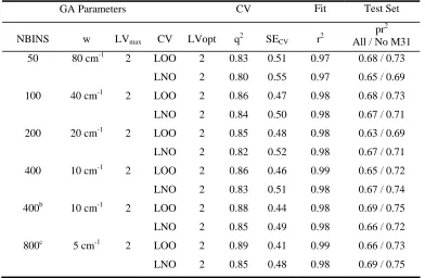
EVA_GA PLS RESULTS: STEROID DATASET

GA Parametersa CVb Fitb Test Set b

RULEc LVmax CV RULEd LVopt q2 SECV r2

pr2 All / No M31 5%_RULE 3 LOO BOTH 2 0.84 0.49 0.98 0.68 / 0.72

LNO BOTH 2 0.82 0.53 0.98 0.66 / 0.70

2 LOO BOTH 2 0.86 0.47 0.98 0.68 / 0.73

LNO BOTH 2 0.84 0.50 0.98 0.67 / 0.71

1 LOO BOTH 1 0.83 0.50 0.96 0.65 / 0.70

LNO BOTH 1 0.80 0.53 0.95 0.65 / 0.70

SECV_MIN 3 LOO SECV_MIN 2e 0.86 0.47 0.99 0.68 / 0.74 5%_RULE 1f 0.83 0.51 0.96 0.67 / 0.71

LNO SECV_MIN 2 0.83 0.51 0.98 0.65 / 0.71

5%_RULE 1 0.80 0.53 0.96 0.63 / 0.68

2 LOO SECV_MIN 2 0.86 0.47 0.99 0.64 / 0.70 5%_RULE 1 0.83 0.50 0.97 0.63 / 0.68

LNO SECV_MIN 2 0.83 0.51 0.98 0.63 / 0.68 5%_RULE 1 0.80 0.54 0.96 0.62 / 0.65

MAX_Q2 3 LOO SECV_MIN 3f 0.86 0.48 0.99 0.63 / 0.69 5%_RULE 1 0.80 0.53 0.96 0.62 / 0.66

LNO SECV_MIN 2 0.82 0.52 0.98 0.65 / 0.70 5%_RULE 1 0.79 0.55 0.95 0.62 / 0.66

2 LOO SECV_MIN 2 0.86 0.46 0.98 0.65 / 0.71 5%_RULE 1 0.83 0.49 0.96 0.63 / 0.68

LNO SECV_MIN 2 0.82 0.52 0.98 0.66 / 0.71 5%_RULE 1 0.79 0.54 0.96 0.64 / 0.69

a

Default GA parameters unless otherwise stated; R = {1, 2, 3, 4, 5}.

b

All PLS statistics are for descriptors derived from Vopt and are mean values taken from 5 GA runs. c

Rule used to select LVopt and thus the chromosome fitness score (q2) during evolution of the GA. d

Rule used to select LVopt and thus the final PLS statistics for Vopt.as distinct from c. e

LVopt = 3 for 2 runs. f

TABLE 5

EVA_GA PLS RESULTS: STEROID DATASET: EFFECT OF MAX_CYCLESa

GA Parameters CV Fit Test Set

MAX_CYCLESb LVmax CV LVopt q2 SECV r2

pr2 All / No M31 50 2 LOO 2 0.84 0.50 0.97 0.66 / 0.70

100 2 LOO 2 0.86 0.47 0.98 0.68 / 0.73

200 2 LOO 2 0.87 0.46 0.98 0.66 / 0.70

400 2 LOO 2 0.85 0.48 0.98 0.69 / 0.73

1000 2 LOO 2 0.87 0.45 0.98 0.67 / 0.72

a

See footnotes to Table 4 for further information; R = {1, 2, 3, 4, 5}.

b

TABLE 6

EVA_GA PLS RESULTS: STEROID DATASET: ALTERNATIVE BIN WIDTHSa

GA Parameters CV Fit Test Set

NBINS w LVmax CV LVopt q2 SECV r2

pr2 All / No M31 50 80 cm-1 2 LOO 2 0.83 0.51 0.97 0.68 / 0.73

LNO 2 0.80 0.55 0.97 0.65 / 0.69

100 40 cm-1 2 LOO 2 0.86 0.47 0.98 0.68 / 0.73

LNO 2 0.84 0.50 0.98 0.67 / 0.71

200 20 cm-1 2 LOO 2 0.85 0.48 0.98 0.63 / 0.69

LNO 2 0.82 0.52 0.98 0.67 / 0.71

400 10 cm-1 2 LOO 2 0.86 0.46 0.99 0.65 / 0.72

LNO 2 0.83 0.51 0.98 0.67 / 0.74

400b 10 cm-1 2 LOO 2 0.88 0.44 0.98 0.69 / 0.75

LNO 2 0.85 0.49 0.98 0.66 / 0.72

800c 5 cm-1 2 LOO 2 0.89 0.41 0.99 0.66 / 0.73

LNO 2 0.85 0.48 0.98 0.69 / 0.75

a

See footnotes to Table 4 for further information; R = {1, 2, 3, 4, 5}.

b

MAX_CYCLES = 400. c

TABLE 7

EVA_GA PLS RESULTS: STEROID DATASET: ALTERNATIVE R SETSa

GA Parameters CV Fit Test Set

R LVmax CV LVopt q2 SECV r2

pr2 All / No M31 {1, 2, 3, 4, 5} 2 LOO 2 0.86b 0.47 0.98c 0.68 / 0.73

LNO 2 0.84 0.50 0.98 0.67 / 0.71

{2, 3, 4, 5, 6} 2 LOO 2 0.84 0.50 0.97 0.67 / 0.72

LNO 2 0.81 0.54 0.97 0.66 / 0.71

{2, 3, 4} 2 LOO 2 0.79 0.57 0.97 0.68 / 0.73

LNO 2 0.79 0.57 0.98 0.68 / 0.72

1 LOO 1 0.76 0.59 0.95 0.62 / 0.68

LNO 1 0.77 0.57 0.95 0.64 / 0.69

{3, 4, 5, 8, 10} 3 LOO 2 0.85 0.47 0.97 0.61 / 0.65

LNO 2 0.83 0.51 0.96 0.65 / 0.70

2 LOO 2 0.86 0.47 0.97 0.64 / 0.68

LNO 2 0.83 0.51 0.97 0.62 / 0.66

1 LOO 1 0.79 0.54 0.93 0.62 / 0.68

LNO 1 0.79 0.55 0.93 0.61 / 0.68

{4, 8, 10, 20, 30} 3 LOO 3 0.90 0.40 0.98 0.25 / 0.42

LNO 3 0.87 0.45 0.98 0.27 / 0.41

2 LOO 2 0.86d 0.45 0.95e 0.39 / 0.52

LNO 2 0.85 0.48 0.95 0.45 / 0.60

1 LOO 1 0.82 0.51 0.91 0.47 / 0.59

LNO 1 0.80 0.54 0.91 0.49 / 0.59

a

See footnotes to Table 4 for further information. b

Chance correlation estimates, p, for q2 are 0.0007 (LV1) and 0.0006 (LV2) (mean values for the five GA runs).

c

Chance correlation estimates, p, for r2 are 0 (LV1 and LV2). d

Chance correlation estimates, p, for q2 are 0.021 (LV1) and 0.0005 (LV2).

e

TABLE 8

STEROIDS: ALTERNATIVE TRAINING AND TEST SET DESIGNS

Classical EVA EVA_GA1

Design σopt LOO/LNO q 2

LVopt r2 pr

2

All / No M31 LVmax LOO q

2

LVopt r2 pr

2

All / No M31

Aa 4 cm-1 0.55 / 0.54 1 0.89 0.51 / 0.57 2 0.71 1 0.96 0.50 / 0.55

Bb 4 cm-1 0.69 / 0.66 2 0.99 0.69 / 0.70 2 0.81 2 0.99 0.66 / 0.66

1

Default GA parameters: models selected according to 5%_RULE; R = { 1, 2, 3, 4, 5}. a

ALL 31 compounds retained: TG = {L4, H6, H7, L9, L13, L18, H22, H23, M26, M27, H30}; M = 11; 20 Test compounds. b

TABLE 9

MELATONIN RECEPTOR LIGANDS: DETAILED COMFA PLS RESULTS.

CoMFA Settings Training Set Test Set pr2

Model Grid Resolution Scaling LOO CV q2 SECV Fitted r 2

All Excl. Z55/56

Literature 2Å not known 0.80 (5)a 0.61 0.97 0.76 not known

Supplied 2Å

1Å None Block None Block 0.65 (3) 0.66 (3)

0.69 (3)b 0.64 (2) 0.76 0.75 0.72 0.76 0.84 0.88 0.86c 0.79 0.68 0.67 0.72 0.68 0.67 0.58 0.71 0.64

CVQ2-GRS [8] q 2

cut-off = 0.1d

q2 cut-off = 0.3d

None None 0.70 (3) 0.67 (3) 0.71 0.74 0.87 0.84 0.74 0.72 0.72 0.65

Aggregate 2Å None

0.58 − 0.81f

mean 0.69 ncg

0.72 − 0.97f mean 0.87

0.43 − 0.88f mean 0.70

0.13 − 0.88f 0.67

Reorientatione

1Å None

0.67 − 0.76f

mean 0.72 ncg

0.85 − 0.97f mean 0.93

0.66 − 0.80f mean 0.73

0.53 − 0.76f 0.67

a

Model LVopt picked on the basis of the (coincident) largest q 2

and smallest SECV [20]. b

Random permutation: for LOO q2, p = 2.2 × 10-5. c Random permutation: for fitted r2, p = 2.2 × 10-6. d

Cut-off value for q2 using which sub-regions are excluded from the final CoMFA; a 1 Å grid resolution is used throughout. e

See main text for details for reorientations used. f Minimum and maximum observed values. g

TABLE 10

CLASSICAL EVA PLS STATISTICS: MELATONIN DATASET

CV Fitted Model Test Set pr2

Parameters RULE LVopt

q2 LOO / LNOa

SECV

LOO / LNOa pb r2 SE pb All

Excl. Z55/56

σ = 10 cm-1 5%_RULE 2 0.46/ 0.44 0.93 / 0.95 0.0005 0.79 0.58 0.0e 0.66 0.81

SECV_MIN 5 0.54 / c 0.90 / c 0.0026 0.95 0.29 0.0e 0.66 0.82

MAX_Q2d 8 0.58 / 0.53 0.90 / 0.94 0.0043 0.98 0.19 0.0e 0.43 0.60

a

Mean of 200 runs of LNO CV where G = 7. b

For both LOO q2 and fitted r2 p is an estimate of the probability of chance correlation based upon 1,000 random permutations of Y.

c

Two LVs were optimal using LNO CV. d

This also corresponds to the overall q2 maximum where ten LVs are extracted. e

TABLE 11

EVA_GA PLS RESULTS: MELATONIN DATASET: ALTERNATIVE R SETSa

GA Parameters CV Fit Test Set

R LVmax CV RULEb LVopt q2 SECV r2

pr2 All / No Z55/56

R1 = {3, 5, 8, 10, 12} 5 LOO SECV_MIN 5d 0.70 0.72 0.96 0.58 / 0.79

5%_RULE 4h 0.69 0.73 0.95 0.58 / 0.80

LNO SECV_MIN 2i 0.61 0.80 0.88 0.74 / 0.87

5%_RULE 2g 0.61 0.80 0.87 0.76 / 0.90

3 LOO BOTH 3j 0.65 0.76 0.90 0.72 / 0.89

LNO BOTH 2f 0.61 0.79 0.88 0.77 / 0.89

2 LOO BOTH 2 0.64 0.76 0.87 0.76 / 0.87

LNO BOTH 2 0.61 0.80 0.86 0.75 / 0.88

1 LOO n/a 1 0.58 0.82 0.75 0.65 / 0.83

LNO n/a 1 0.55 0.84 0.74 0.63 / 0.80

R2 = {2, 4, 6, 8, 10} 5 LOO SECV_MIN 5c 0.70 0.72 0.98 0.63 / 0.80

5%_RULE 4d 0.69 0.73 0.95 0.66 / 0.83

LNO BOTH 2e 0.64 0.77 0.89 0.74 / 0.88 3 LOO BOTH 3d 0.67 0.74 0.92 0.76 / 0.89

LNO SECV_MIN 2f 0.62 0.79 0.89 0.72 / 0.86

5%_RULE 2g 0.61 0.79 0.88 0.73 / 0.86

2 LOO BOTH 2 0.65 0.76 0.88 0.74 / 0.87

LNO BOTH 2 0.63 0.78 0.87 0.74 / 0.86

1 LOO n/a 1 0.59 0.80 0.76 0.67 / 0.80

LNO n/a 1 0.58 0.81 0.76 0.65 / 0.78

R3 = {5, 10, 15, 20, 30} 3 LOO BOTH 3 0.68 0.73 0.91 0.69 / 0.77

LNO BOTH 3 0.63 0.78 0.90 0.64 / 0.80

2 LOO BOTH 2 0.63 0.78 0.83 0.65 / 0.80

LNO BOTH 2 0.58 0.82 0.82 0.64 / 0.80

1 LOO n/a 1 0.55 0.85 0.70 0.50 / 0.74

LNO n/a 1 0.53 0.86 0.68 0.47 / 0.74

a

See footnotes to Table 4 for further information. b

Rule used to select LVopt and thus the final PLS statistics for Vopt.− not an EVA_GA parameter. c

For two solutions LVopt = 4. d

For one solution LVopt = 2. e

For one solution LVopt = 4. f

For two solutions LVopt = 3. g

For one solution LVopt = 3. h

For one solution LVopt = 2; for one solution LVopt = 5.

i

For one solution LVopt = 5. j

TABLE 12

EVA_GA PLS RESULTS: MELATONIN DATASET: EFFECT OF MAX_CYCLESa

GA Parameters CV Fit Test Set

MAX_CYCLESc LVmax CV LVopt q2 SECV r2

pr2 All / No Z55/56

50 3 LOO 3c 0.64 0.77 0.90 0.74 / 0.89

100 3 LOO 3c 0.65 0.76 0.90 0.72 / 0.89

200 3 LOO 3c 0.67 0.74 0.91 0.74 / 0.90

400 3 LOO 3 0.68 0.73 0.92 0.73 / 0.90

1000 3 LOO 3 0.70 0.71 0.92 0.72 / 0.90

a

See footnotes to Table 4 for further information; R = {3, 5, 8, 10, 12}.

b

Maximum iterations of the GA − each run was started separately with a different random seed and the CONV_CRIT set so that convergence was not reached.

c

TABLE 13

EVA_GA PLS RESULTS: MELATONIN DATASET: ALTERNATIVE BIN WIDTHSa

GA Parameters CV Fit Test Set

NBINS w LVmax CV LVopt q2 SECV r2

pr2 All / No Z55/56

50 80 cm-1 3 LOO 3b 0.61 0.80 0.90 0.70 / 0.83

100 40 cm-1 3 LOO 3c 0.65 0.76 0.90 0.72 / 0.89

200 20 cm-1 3 LOO 3 0.71 0.70 0.95 0.72 / 0.88

400 10 cm-1 3 LOO 3 0.75 0.65 0.96 0.73 / 0.81

800 5 cm-1 3 LOO 3 0.80 0.58 0.98 0.68 / 0.86

800d 5 cm-1 3 LOO 3 0.91 0.39 0.99 0.67 / 0.81

a

See footnotes to Table 4 for further information; R = {3, 5, 8, 10, 12}.

b

For one solution LVopt = 2.

c

For two solutions LVopt = 2. d

Fig. 1. Histogram summarising the number of fundamental NMFs found in different regions of the IR spectrum (melatonin receptor ligand training dataset, bin widths (w) of 40 cm-1).

0 50 100 150 200 250

Wavenumber ranges (cm-1) Counts

200 400 600 800 1000 1200 1400 1600 1800 2000 2200 2400 2600 2800 3000 3200 3400 3600 3800 4000 0

???????????????? Skeletal region ???????????????? ??????? Functional Group ??????? ??????????? Hydrogen Stretch ????????????

Fig. 2. Example of the different kernel widths and shapes obtained after expansion with selected Gaussian standard deviation (σ) values (after scaling to unit maximum amplitude) for a single hypothetical frequency at 29 cm-1.

0.0 0.2 0.4 0.6 0.8 1.0

1 5 9 13 17 21 25 29 33 37 41 45 49 53 57

Wavenumber (cm-1) f(x)

40 cm-1

20 cm-1

10 cm-1

5 cm-1

2 cm-1

Fig. 3. Overview of GA routine.

Initialise Population

Evaluate Fitness (PLS)

Reproduce 1. Select parents 2. Cross-over 3. Mutation

Solution(s) Iterate

until CONVERGENCE

or MAX_CYCLES

Fig. 4. Melatonin training and test set compounds with CoMFA superposition centresa. N N H R1 R3 R2 C R4 O H Indoles (T01-T09) * * * * * C R4 O H

Naphthalenes: Type I (T10-T22)

R2 N R1 * * * * * C R4 O H

Naphthalenes: Type II (T23-T32, Z51)

N R2 R1 R3 * * * * * C R4 O H

Tricyclics (T33-T34, Z52)

N

MeO

* * *

* *

C CH₃

C R4 O H

Benzenes (T37-T46, Z53-Z57)

N

R1

R2

* * _*

* *

C CH₃

O H

Quinolinic (Z49)

N N

*

H

* *

* *

a

TG and test set compounds prefixed with "T" and "Z" respectively.

C O H

Naphthalene-like (Z50)

R2

N Et

MeO

* * *