White Rose Research Online URL for this paper:
http://eprints.whiterose.ac.uk/1430/
Article:
Stone, J.V. (2001) Blind source separation using temporal predictability. Neural
Computation, 13 (7). pp. 1559-1574. ISSN 0899-7667
https://doi.org/10.1162/089976601750265009
[email protected] https://eprints.whiterose.ac.uk/ Reuse
Unless indicated otherwise, fulltext items are protected by copyright with all rights reserved. The copyright exception in section 29 of the Copyright, Designs and Patents Act 1988 allows the making of a single copy solely for the purpose of non-commercial research or private study within the limits of fair dealing. The publisher or other rights-holder may allow further reproduction and re-use of this version - refer to the White Rose Research Online record for this item. Where records identify the publisher as the copyright holder, users can verify any specific terms of use on the publisher’s website.
Takedown
If you consider content in White Rose Research Online to be in breach of UK law, please notify us by
Blind Source Separation Using Temporal Predictability
James V. Stone
Psychology Department, Sheffield University, Sheffield, S10 2UR, England
A measure of temporal predictability is defined and used to separate lin-ear mixtures of signals. Given any set of statistically independent source signals, it is conjectured here that a linear mixture of those signals has the following property: the temporal predictability of any signal mixture is less than (or equal to) that of any of its component source signals. It is shown that this property can be used to recover source signals from a set of linear mixtures of those signals by finding an un-mixing matrix that maximizes a measure of temporal predictability for each recovered signal. This matrix is obtained as the solution to a generalized eigenvalue
problem; such problems have scaling characteristics ofO(N3), whereN
is the number of signal mixtures. In contrast to independent component analysis, the temporal predictability method requires minimal assump-tions regarding the probability density funcassump-tions of source signals. It is demonstrated that the method can separate signal mixtures in which each mixture is a linear combination of source signals with supergaussian, sub-gaussian, and gaussian probability density functions and on mixtures of voices and music.
1 Introduction
Almost every signal measured within a physical system is actually a mixture of statistically independent source signals. However, because source signals are usually generated by the motion of mass (e.g., a membrane), the form of physically possible source signals is underwritten by the laws that govern how masses can move over time. This suggests that the most parsimonious explanation for the complexity of a given observed signal is that it consists of a mixture of simpler source signals, each from a different physical source. Here, this observation has been used as a basis for recovering source signals from mixtures of those signals.
Consider two people speaking simultaneously, with each person a dif-ferent distance from two microphones. Each microphone records a linear mixture of the two voices. The two resultant voice mixtures exemplify three universal properties of linear mixtures of statistically independent source signals:
1. Temporal predictability (conjecture)—The temporal predictability
(formally defined later) of any signal mixture is less than (or equal to) that of any of its component source signals.
2. Gaussian probability density function—The central limit theorem
ensures that the extent to which the probability density function (pdf) of any mixture approximates a gaussian distribution is greater than (or equal to) any of its component source signals.
3. Statistical Independence—The degree of statistical independence
be-tween any two signal mixtures is less than (or equal to) the degree of independence between any two source signals.
Property 2 forms the basis of projection pursuit (Friedman, 1987), and properties 1 and 2 are critical assumptions underlying independent com-ponent analysis (ICA) (Jutten & H´erault, 1988; Bell & Sejnowski, 1995). All three properties are generic characteristics of signal mixtures. Unlike prop-erties 2 and 3, property 1 (temporal predictability) has received relatively little attention as a basis for source separation.
However, temporal predictability has been used to augment conven-tional source separation methods, such as ICA.1These conventional source
separation methods are defined in terms of model pdfs and their corre-sponding cumulative density functions (cdfs) of source signals. Such meth-ods are invariant with respect to temporal permutations of signals. For convenience, these methods will be referred to as cdf-based blind source separation (BSS cdf) methods. Specifically, Pearlmutter and Parra (1996) in-corporate a linear predictive coding (LPC) model into Bell and Sejnowski’s ICA method. This is achieved by augmenting the conventional ICA un-mixing matrixW with extra parameters, which are coefficients of a LPC model. The resulting “contextual ICA” method encourages extraction of source signals that conform to both the LPC model and the high-kurtosis pdf model implicit in ICA. Attias (2000) describes a method for augment-ing independent factor analysis with a first-order hidden Markov model in order to model temporal dependences within each source signal. The meth-ods described in both Pearlmutter and Parra (1996) and Attias (2000) are demonstrated on signals that cannot be separated by ICA alone. More re-cently, Hyv¨arinen (2000) described complexity pursuit, a method in which ICA is augmented with a measure of the time dependencies of extracted sources.2However, each of these three methods requires the use of itera-tive, gradient-ascent techniques in order to locate maxima of a nonlinear merit function.
The Bussgang techniques surveyed in Bellini (1994) can be shown to equalize correlations between a signal and a time-delayed version of that
1The method described in Bell & Sejnowski (1995). Bell and Sejnowski (1995) is used
as a reference point for conventional ICA methods in this article.
signal, for a specific value of delay. However, Bussgang techniques also require a nonlinear function to be chosen, which is analogous to the cdf used in ICA. As with ICA, the quality of solutions can depend critically on the form chosen for this nonlinear function (Cardoso, 1998).
Wu and Principe (1999) describe a BSS cdf technique for separation of source signals with nongaussian pdfs, without prior knowledge of the pdfs of source signals. In common with ICA, the method is based on the obser-vation that source signals tend to be nongaussian. In contrast to ICA, source signals are recovered by maximizing a quadratic measure of the difference between each extracted signal and a gaussian signal with the same standard deviation as the extracted signal.
One source separation method that does not explicitly rely on the pdf of extracted signals is described in Molgedey and Schuster (1994). These authors implicitly assume that a set of source signals is uncorrelated at two different time lags:L = 0 andL = 1t. This yields a general eigenvalue problem, so that the solution matrix is unique and readily obtainable using standard eigenvalue routines. One practical drawback is the method’s sen-sitivity to the chosen value of1t. For example, if one of two source signals is periodic with periodθ=1t, then the solutions to the eigenvalue problem become degenerate, so that source separation fails.
In this article, a method explicitly based on a simple measure of tempo-ral predictability is introduced. The main contribution of this article is to demonstrate that maximizing temporal predictability alone can be sufficient for separating signal sources. No formal proof is given of the temporal pre-dictability conjecture stated in previously in this section, the main purpose being to demonstrate the utility associated with this conjecture. Although counterexamples to this informal conjecture are easy to construct, a formal definition of the conjecture is robust with respect to such counterexamples (see section 1.4). Moreover, results presented here suggest that the conjecture holds true for many physically realistic signals, such as voices and music.
1.1 Problem Definition and Temporal Predictability. Consider a set of
Kstatistically independent source signals s = {s1 | s2 | · · · | sK}t, where theith row in s is a signalsimeasured atntime points (the superscriptt denotes the transpose operator). It is assumed throughout this article that source signals are statistically independent, unless stated otherwise. A set ofM ≥ K linear mixturesx = {x1 | x2 | · · · | xM}t of signals ins can be formed with anM×Kmixing matrixA:x=As. If the rows ofAare linearly independent,3 then any source signals
ican be recovered from x with a 1×MmatrixWi:si = Wix. The problem to be addressed here consists in finding an unmixing matrixW= {W1 |W2| · · · |WK}tsuch that each row
3This condition can be satisfied (for instance) by placing each ofKspeakers a different
vectorWi recovers a different signalyi, whereyi is a scaled version of a source signalsi, forK=Msignals.
1.2 A Solution Strategy. The method for recovering source signals is
based on the following conjecture: the temporal predictability of a signal mixturexiis usually less than that of any of the source signals that contribute toxi. For example, the waveform obtained by adding two sine waves with different frequencies is more complex than either of the original sine waves. This observation is used to define a measureF(Wi,x)of temporal pre-dictability, which is then used to estimate the relative predictability of a signalyirecovered by a given matrixWi, whereyi=Wix. If source signals are more predictable than any linear mixtureyiof those signals, then the value ofWi, which maximizes the predictability of an extracted signalyi, should yield a source signal (i.e.,yi=csi, wherecis a constant).
An information-theoretic analysis of the function F proves that max-imizing the temporal predictability of a signal amounts to differentially maximizing the power of Fourier components with the lowest (nonzero) frequencies (see Stone, 1996b, Stone, 1999). The functionFis invariant with respect to the power of low-frequency components in signal mixtures and therefore tends to amplify differentially even very low power components, which have the lowest (nonzero) temporal frequency.
1.3 Measuring Signal Predictability. The definition of signal
predictabil-ityFused here is:
F(Wi,x)=log
V(Wi,x) U(Wi,x)
=log Vi
Ui
=log
Pn
τ=1(yτ−yτ)2
Pn
τ=1(yτ˜ −yτ)2
, (1.1)
whereyτ =Wixτis the value of the signalyat timeτ, andxτis a vector ofK signal mixture values at timeτ. The termUireflects the extent to whichyτ is predicted by a short-term moving averageyτ˜ of values iny. In contrast, the termViis a measure of the overall variability iny, as measured by the extent to whichyτis predicted by a long-term moving averageyτof values iny. The predicted valuesyτ˜ andyτofyτ are both exponentially weighted sums of signal values measured up to time(τ−1), such that recent values have a larger weighting than those in the distant past:
˜
yτ =λSy(τ˜ −1)+(1−λS)y(τ−1): 0≤λS≤1
yτ =λLy(τ−1)+(1−λL)y(τ−1): 0≤λL≤1. (1.2)
The half-lifehLofλLis much longer (typically 100 times longer) than the corresponding half-lifehSofλS. The relation between a half-lifehand the parameterλis defined asλ=2−1/h.
Uwould result in a DC signal. In both cases, trivial solutions would be obtained forWibecauseVican be maximized by setting the norm ofWito be large, andUcan be minimized by settingWi =0. In contrast, the ratio Vi/Uican be maximized only if two constraints are both satisfied: (1)yhas a nonzero range (i.e., high variance) and (2) the values inychange slowly over time. Note also that the value ofFis independent of the norm ofWi, so that only changes in the direction ofWiaffect the value ofF4.
1.4 Redefining Signal Predictability. One counterexample to the
tem-poral predictability conjecture is as follows. Consider two sine wave source signalss1ands2with the same period such thats2=s1+π. The signal
mix-tures=s1+s2is zero at all time points and is therefore quite predictable.
Whilesis intuitively predictable, the operational definition of predictabil-ityFused here is robust with respect to such counterexamples. Specifically, the value of the functionFis undefined forsbecause ifs=0 everywhere, thenVi=Ui =0 andF=log 0/0. Conversely, if the frequencies ofs1and
s2are not exactly the same, then the value ofFis no longer undefined.
The informal temporal predictability conjecture can now be restated for-mally in terms of the functionF, as follows: if the value ofFassociated with a signal mixturexiis not undefined, then the value ofFof each mixture is greater than (or equal to) the value ofFof each source signal in that mixture.
2 Extracting Signals by Maximizing Signal Predictability
2.1 Extracting a Single Signal. Consider a scalar signal mixtureyiformed
by the application of a 1×MmatrixWito a set ofK =Msignalsx. Given thatyi=Wix, equation (1.1) can be rewritten as
F=logWiCW t i WiCW˜ it
, (2.1)
whereCis anM×Mmatrix of long-term covariances between signal mix-tures andC˜is a corresponding matrix of short-term covariances. The long-term covarianceCijand the short-term covarianceC˜ijbetween theith and jth mixtures are defined as
˜ Cij=
n
X
τ
(xiτ− ˜xiτ)(xjτ− ˜xjτ)
Cij= n
X
τ
(xiτ−xiτ)(xjτ−xjτ). (2.2)
4Previous experience with iterative gradient ascent onFshows that the length ofW
i
Note thatC˜andCneed to be computed only once for a given set of signal mixtures and that the terms(xiτ−xiτ)and(xiτ− ˜xiτ)can be precomputed using fast convolution operations, as described in Eglen, Bray, and Stone (1997).
Gradient ascent onFwith respect toWicould be used to maximizeF, thereby maximizing the predictability ofyi. The derivative ofFwith respect toWiis
∇WiF= 2Wi Vi
C−2Wi Ui
˜
C. (2.3)
One optimization procedure (not used here) would consist of iteratively updatingWiuntil a maximum ofFis located:Wi=Wi+η∇WiF, whereηis
a small constant (typically,η=0.001).
Note that the functionFis a ratio of quadratic forms. Therefore,Fhas ex-actly one global maximum and exex-actly one global minimum, with all other critical points being saddle points (Borga, 1998). This implies that gradient ascent is guaranteed to find the global maximum inF. Unfortunately, re-peated application of the above procedure to a single set of mixtures extracts the same (most predictable) source signal. While this can be prevented by us-ing procedures such as Gram-Schmidt orthonormalization, a more elegant method for extracting all of the sources simultaneously exists, as described next.
2.2 Simultaneous Source Separation. The gradient ofFis zero at a
so-lution where, from equation (2.3),
WiC= Vi Ui
WiC˜. (2.4)
Extrema inFcorrespond to values ofWithat satisfy equation (2.4), which has the form of a generalized eigenproblem (Borga, 1998). Solutions forWi can therefore be obtained as eigenvectors of the matrix(C˜−1C), with
corre-sponding eigenvaluesγi=Vi/Ui. As noted above, the first such eigenvector defines a maximum inF, and each of the remaining eigenvectors defines saddle points inF.
Note that eigenproblems have scaling characteristics ofO(N3), whereN
is the number of signal mixtures. The matrixW can be obtained using a generalized eigenvalue routine. Results presented in this article were ob-tained using the Matlab eigenvalue functionW =eig(C,C˜). AllKsignals can then be recovered:y=Wx, where each row ofycorresponds to exactly one extracted signalyi.
for reducingMconsists of using principal component analysis (PCA). PCA is used to reduce the dimensionality of the signal mixtures by discarding eigenvectors ofxthat have eigenvalues close to zero. However, in this article, only mixtures for whichK=Mare analyzed.
2.3 A Physical Interpretation. The solutions found by the method are
the eigenvectors(W1,W2, . . . ,WM)of the matrix(C˜−1C). These eigenvectors are orthogonal in the metricsCandC˜:
WiCW˜ jt =0
WiCWjt =0, (2.5)
where,
WiCW˜ jt =
X
τ
(yiτ− ˜yiτ)(yjτ− ˜yjτ)
WiCWjt =
X
τ
(yiτ−yiτ)(yjτ−yjτ). (2.6)
Given equations (2.5), a simple and physically realistic interpretation of the method can be demonstrated. Consider the short-term and long-term half-life parametershSandhLin the limits(hS →0)and(hL → ∞). First, in the limit(hS → 0), the short-term mean is yτ˜ ≈ yτ−1, and therefore (yτ − ˜yτ) ≈ dyτ/dτ = y′
τ. Second, if y has zero mean, then in the limit
(hL→ ∞), the long-term meany≈0, and therefore(yτ−yτ)≈yτ. In these limiting cases, equations (2.5) and (2.6) imply that
E[y′
iy′j]=0
E[yiyj]=0, (2.7)
whereE[ ] denotes an expectation value. Thus, one interpretation of the method is that each signalyi=Wixis uncorrelated with every other signal yj =Wjx,andthe temporal derivativey′i =Wix′of each extracted signal is uncorrelated with the temporal derivativey′
j=Wjx′of every other extracted signal, wherex′is a vector variable that is the temporal derivative of the
mixturesx. Critically, if two signalsyiandyjare statistically independent then the conditions specified in equation (2.7) are met. Therefore, mixtures of independent signals are guaranteed to be separable by the method, at least in the limiting cases specified above.
3 Results
Table 1: Correlation Magnitudes Between Source Signals and Signals Recovered from Mixtures of Source Signals with Different pdfs.
Source Signals Signals
Recovered s1 s2 s3
y1 0.000 0.001 1.000 y2 1.000 0.000 0.000 y3 0.042 0.999 0.002
K signal mixtures, using aK×K mixing matrix, and these M mixtures were used as input to the method. Each mixture signal was normalized to have zero-mean and unit variance. Each mixing matrix was obtained using the Matlabrandnfunction. The short-term and long-term half-lives defined in equation (1.2) were set tohS = 1 andhL = 9000, respectively. Correlations between source signals and recovered signals are reported as absolute values. Results were obtained in under 60 seconds on a Macintosh G3 (233 MHz) for all experiments reported here, using nonoptimized Matlab code. In each case, an un-mixing matrix was obtained as the solution to a generalised eigenvalue problem using the Matlab eigenvalue function W=eig(C,C˜).
3.1 Separating Mixtures of Signals with Different Pdfs. Three source
signalss = {s1 | s2 | s3}t are displayed in Figure 2: (1) a supergaussian
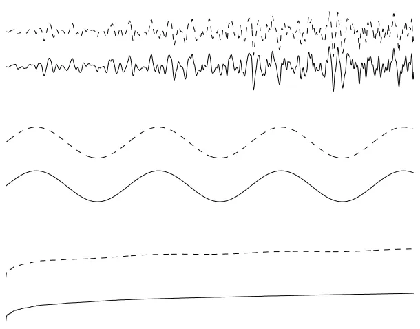
signal (the sound of a gong), (2) a subgaussian signal (a sine wave), and (3) a gaussian signal. Signal 3 was generated using therandnprocedure in Matlab, and temporal structure was imposed on the signal by sorting its values in ascending order. These three signals were mixed using a random matrixAto yield a set of three signal mixtures:x=As. Each signal consisted of 3000 samples; the first 1000 samples of each mixture are shown in Figure 1. The correlations between source signals and recovered signals are given in Table 1. The three recovered signals each had a correlation ofr>0.99, with only one of the source signals, and other correlations were close to zero. Note that the mixtures used here do not include any temporal delays or echoes.
3.2 Separating Mixtures of Sounds. For each experiment reported here,
50,000 data points were sampled at a rate 44,100 Hz, using a microphone to record different voices from a VHF radio onto a Macintosh computer. Two sets of eight sounds were recorded: male and female voices and classical music, with and without singing.
Figure 1: Three signal mixtures used as input to the method. See Figure 2 for a description of the three source signals used to synthesize these mixtures. Only the first 1000 of the 9000 samples used in experiments are shown here. The ordinal axis displays signal amplitude.
of original (source) voice amplitudes and the signals recovered from a set of four mixtures (not shown) are shown in Figure 3. Note that correlations are approximatelyr = 0.99. With correlations this high, it is not possible to hear the difference between the original and recovered speech signals. A correlation of 0.956 was found between source 8 and recovered signal 3; this represents the worst performance of the method out of all data sets described in this article.
Table 2: Correlation Magnitudes Between Each of Four Source Signals and Ev-ery Signal Recovered (y1, . . . ,y4) by the Method.
Source Signals (voices) Signal
Recovered s1 s2 s3 s4
y1 0.097 0.994 0.028 0.049 y2 0.996 0.081 0.012 0.019 y3 0.002 0.042 0.995 0.095 y4 0.030 0.076 0.101 0.992
[image:10.612.195.379.551.636.2]Figure 2: Three signals with different probability density functions. A super-gaussian gong sound, a subsuper-gaussian sine wave, and sorted super-gaussian noise (see text) are displayed from top to bottom respectively. In each graph, the source signals used to synthesize the mixtures displayed in Figure 1 are shown as a solid line, and corresponding signals recovered from those mixtures are shown as dotted lines. Each source signal and its corresponding recovered signal have been shifted vertically for display purposes. The correlations between source and recovered signals are greater thanr = 0.999 (see Table 1). Only the first 1000 of the 9000 samples used are shown here. The ordinal axis displays signal amplitude.
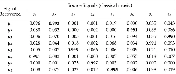
3.2.2 Separating Music. The method was tested on mixtures of eight seg-ments of music. Correlations between each source signal and each recovered signal for eight music segments are given in Table 4. Again, correlations are approximatelyr=0.99, and it is not possible to hear the difference between the original and recovered music signals.
The method seems to be largely insensitive to the values used for the short-term and long-term half-lives defined in equation 1.2, provided the latter is much larger than the former.
3.3 How Maximizing Predictability Can Fail. The method is based on
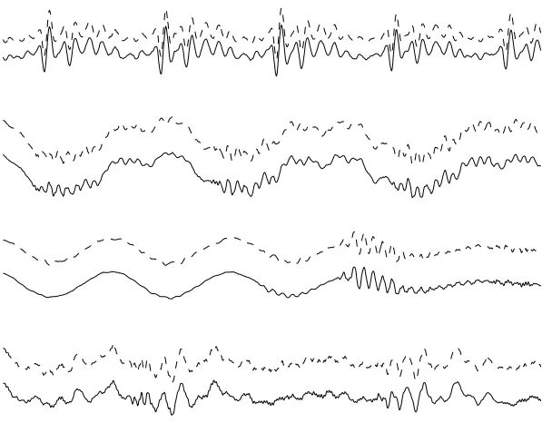
Figure 3: Four voices (two male and two female). In each graph, the source signals used to synthesize four mixtures (not shown) are shown as solid lines, and corresponding signals recovered from these mixtures are in shown as dot-ted lines. Each source signal and its corresponding recovered signal have been shifted vertically for display purposes. The correlations between source and re-covered signals are greater thanr=0.99 (see Table 2). Only the first 1000 of the 50,000 samples used are shown here. The ordinal axis displays signal amplitude.
Table 3: Correlation Magnitudes Between Each of Eight Source Signals and Every Signal Recovered by the Method.
Source Signals (voices) Signal
Recovered s1 s2 s3 s4 s5 s6 s7 s8
y1 0.001 0.008 0.004 0.003 0.028 0.046 0.988 0.143 y2 0.994 0.013 0.003 0.001 0.001 0.017 0.016 0.109 y3 0.179 0.001 0.162 0.011 0.037 0.102 0.134 0.956 y4 0.015 0.012 0.007 0.999 0.024 0.032 0.004 0.004 y5 0.004 0.020 0.993 0.000 0.021 0.008 0.007 0.109 y6 0.010 0.003 0.026 0.018 0.021 0.992 0.044 0.111 y7 0.027 0.999 0.012 0.002 0.000 0.010 0.009 0.002 y8 0.015 0.003 0.027 0.022 0.998 0.020 0.021 0.043
[image:12.612.141.437.513.640.2]Table 4: Correlation Magnitudes Between Each of Eight Source Signals and Every Signal Recovered (y1, . . .y8) by the Method.
Source Signals (classical music) Signal
Recovered s1 s2 s3 s4 s5 s6 s7 s8
y1 0.096 0.993 0.001 0.001 0.019 0.030 0.035 0.043 y2 0.088 0.032 0.000 0.002 0.000 0.991 0.038 0.086 y3 0.006 0.070 0.005 0.001 0.016 0.094 0.085 0.990 y4 0.028 0.044 0.018 0.002 0.068 0.034 0.991 0.093 y5 0.005 0.007 0.998 0.066 0.006 0.009 0.021 0.010 y6 0.995 0.083 0.001 0.008 0.007 0.055 0.018 0.007 y7 0.000 0.001 0.075 0.997 0.002 0.002 0.000 0.000 y8 0.008 0.027 0.022 0.012 0.995 0.006 0.098 0.019
Note: Each source signal has a high correlation with only one recovered signal.
same degree of predictability F, then two eigenvectors Wi and Wj have equal eigenvalues (and are associated with the same critical points inF). Therefore, any vectorWkthat lies in the plane defined byWiandWjalso maximizesF, butWkcannot (in general) be used to extract a source signal. This has been demonstrated (not shown here) by creating two mixtures
x =Asfrom two signalss1 ands2, wheres1is a time-reversed version of
s2. Althoughs1ands2 have different time courses, they share exactly the
same degree of predictabilityFand cannot be extracted from the mixtures
xusing this method.
In practice, signals from different sources (e.g., voices) typically can be separated because each source signal has a unique degree of predictability (i.e., value ofF). Indeed, every set of signals in which each signal is from a physically distinct source (e.g., voices) has been successfully separated in the many experiments used in the preparation of this article.
4 Discussion
sig-nals). The last two have previously been used as a basis for signal separation, and the first has been used to augment source separation (e.g., Pearlmutter & Parra, 1996; Attias, 2000; Porrill, Stone, Berwick, Mayhew, & Coffey, 2000). In this article, only the first property (temporal predictability) has been used to separate signal mixtures.
While the method has a low-order polynomial time complexity ofO(N3),
this does not necessarily imply that it finds solutions more quickly than other source separation methods (see Comon & Chevalier, 2000, for an analysis of the time complexity of ICA methods). However, the fact that each simulation reported here was run in under 60 seconds (on a Macintosh G3) may indicate that the method is reasonably fast. This issue can be resolved only by a direct comparison of different methods on the same data sets. One desirable property of method described in this article is that local extrema are not an issue. This contrasts with other methods for which the existence of local extrema may be difficult to detect (Ding, Hohnson, & Kennedy, 1994).
Of the methods reviewed in section 1, the method that Molgedey and Schuster (1994) described is mathematically most similar to the one de-scribed in this article, inasmuch as both methods involve a generalized eigenvalue problem. As stated in section 1, Molgedey and Schuster implic-itly assume that source signals are uncorrelated at two different time lags. In contrast, one interpretation of the assumptions underlying the method pre-sented here is that source signals are uncorrelatedandtheir corresponding temporal derivatives are also uncorrelated (in the limiting cases specified in ection 2.3). Thus, although both methods can be formulated as generalized eigenvalue problems, the assumptions required by each method regarding the nature of source signals are qualitatively very different.
As defined above, the predictions (yτandyτ˜ ) of each signal valueyτare based on a linear weighted sum of previous values{y}. Natural extensions to this method could involve defining predicted values of yτ as general functions of previous signal values{y}, yielding functionals of the general form
G=log
Pn
τ=1(f({y} −yτ)2
Pn
τ=1(g({y} −yτ)2
. (4.1)
in the development of the method presented here). In particular, the issue of sensor (e.g., microphone) noise has not been addressed in this article, and these more elaborate measures of predictability may be robust with respect to such noise.
It is noteworthy that the principles underlying the method have been used for unsupervised learning in artificial neural networks (Stone, 1996a, 1996b, 1999; Becker & Hinton, 1992; Becker, 1993). This principle is useful for both unsupervised learning and source signal separation precisely because it is based on a fundamental property of the physical world: temporal pre-dictability. However, predictability is not only a property of the temporal domain; an obvious extension (explored in Becker & Hinton, 1992; Eglen et al., 1997; Stone & Bray, 1995) is to apply the principle to the spatial domain. Additionally, the assumptions of temporal or spatial predictability used in the methods just described can be combined in a method that assumes a degree of temporal and spatial predictability. Specifically, methods that maximize predictability in space or predictability in time can be replaced by a method that maximizes predictability over space and time. An analogous spatiotemporal ICA method has been described in Stone, Porrill, Buchel, and Friston (1999).
If all three properties listed above apply to any statistically independent source signals and their mixtures, a method that relies on constraints from all of these properties might be expected to deal with a wide range of signal types. It is widely acknowledged that ICA forces statistical independence on recovered signals, even if the underlying source signals are not indepen-dent. Similarly, the current method may impose temporal predictability on recovered signals even where none exists in the underlying source signals. Therefore, a method that incorporates constraints from all three properties should be relatively insensitive to violations of the assumptions on which the method is based. A framework for incorporating experimentally rele-vant constraints based on physically realistic properties has been formu-lated in the form of weak models (Porrill et al., 2000) and has been used to constrain ICA’s solutions. In particular, the functionFhas the correct form for a weak model and has been shown to improve solutions found by ICA (Stone & Porrill, 1999). Finally, the method described here may be useful in the analysis of medical images and electroencephalogram data.
Acknowledgments
Thanks to J. Porrill for discussions of the generalized eigenvalue method. Thanks to R. Lister, D. Johnston, N. Hunkin, S. Isard, K. Friston, D. Buckley, and two anonymous referees for comments on this article. This research was supported by a Mathematical Biology Wellcome Fellowship (Grant Number 044823).
References
Attias, H. (2000). Independent factor analysis with temporally structured factors. In S. A. Solla, T. K. Leen, & K.-R. M. (Eds.),Advances in neural information processing systems, 12. Cambridge, MA: MIT Press.
Becker, S. (1993). Learning to categorize objects using temporal coherence. In S. J. Hanson, J. Cowan, & C. L. Giles (Eds.),Neural information processing systems, 5(pp. 361–368). San Mateo, CA: Morgan Kaufmann.
Becker, S., & Hinton, G. (1992). Self-organizing neural network that discovers surfaces in random-dot stereograms.Nature,335, 161–163.
Bell, A., & Sejnowski, T. (1995). An information-maximization approach to blind separation and blind deconvolution.Neural Computation,7, 1129–1159. Bellini, S. (1994). Bussgang techniques for blind deconvolution and
equaliza-tion. In S. Haykin (Ed.),Blind deconvolution(pp. 8–59). Englewood Cliffs, NJ: Prentice Hall.
Borga, M. (1998).Learning multidimensional signal processing. Unpublished doc-toral dissertation Linkoping University, Linkoping, Sweden.
Cardoso, J. (1998). On the stability of some source separation algorithms. In Proceddings of Neural Networks for Signal Processing ’98(pp. 13–22). Cambridge, England.
Comon, P., & Chevalier, P. (2000). Blind source separation: Models, concepts, al-gorithms and performance. In S. Haykin (Ed.),Unsupervised adaptive filtering, Vol. 1: Blind source separation(pp. 191–235). New York: Wiley.
Ding, Z., Hohnson, C., & Kennedy, R. (1994). Global convergence issues with lin-ear blind adaptive equalizers. In S. Haykin (Ed.),Blind deconvolution(pp. 60– 115). Englewood Cliffs, NJ: Prentice Hall.
Eglen, S., Bray, A., & Stone, J. (1997). Unsupervised discovery of invariances. Network,8, 441–452.
Friedman, J. (1987). Exploratory projection pursuit.Journal of the American Sta-tistical Association,82(397), 249–266.
Hyv¨arinen, A. (2000). Complexity pursuit: Combining nongaussinity and auto-correlations of signal separation. InProc. Int. Workshop on Independent Com-ponent Analysis and Blind Signal Separation (ICA2000)(pp. 175–180). Helsinki, Finland.
Jutten, C., & H´erault, J. (1988). Independent component analysis versus pca. In Proc. EUSIPCO(pp. 643–646).
Pearlmutter, B., & Parra, L. (1996). A context-sensitive generalization of ica. In In-ternational Conference on Neural Information Processing. Hong Kong. Available online at: http://www.cs.unm.edu/∼bap/publications.html#journal. Pincus, S., & Singer, B. (1996). Randomness and degrees of irregularity.
Proceed-ings of the National Academy of Sciences USA,93, 2083–2088.
Porrill, J., Stone, J. V, Berwick, J., Mayhew, J., & Coffey, P. (2000). Analysis of optical imaging data using weak models and ICA. In M. Girolami (Ed.), Advances in independent component analysis. Berlin: Springer-Verlag.
Stone, J. V (1996a). A canonical microfunction for learning perceptual invari-ances.Perception,25(2), 207–220.
Stone, J. V (1996b). Learning perceptually salient visual parameters through spatiotemporal smoothness constraints.Neural Computation,8(7), 1463–1492. Stone, J. V (1999). Learning perceptually salient visual parameters using spa-tiotemporal smoothness constraints. In G. Hinton & T. Sejnowski (Eds.), Un-supervised learning: Foundations of neural computation(pp. 71–100). Cambridge, MA: MIT Press.
Stone, J. V, & Bray, A. (1995). A learning rule for extracting spatio-temporal invariances.Network,6(3),1–8.
Stone, J. V, & Porrill, J. (1999).Regularisation using spatiotemporal independence and predictability(Tech. Rep. No. 201). Sheffield: Sheffield University.
Stone, J. V, Porrill, J., Buchel, C., & Friston, K. (1999). Spatial, temporal, and spa-tiotemporal independent component analysis of FMRI data. In K. V. Mardia, R. G. Aykroyd, & I. L. Dryden (Eds.),Proceedings of the 18th Leeds Statistical Re-search Workshop on Spatial-Temporal Modelling and Its Applications(pp. 23–28). Leeds: Leeds University Press.
Wu, H., & Principe, J. (1999). A gaussianity measure for blind source separation insensitive to the sign of kurtosis. InNeural Networks for Signal Processing IX: Proceedings of the 1999 Signal Processing Society Workshop(pp. 58–66).