Answers (Chapter 12) pdf

Full text

(1)Discovering Statistics Using SPSS: Chapter 12. Chapter 12: Answers Task 1 I am going to extend the example from the previous chapter (advertising and different imagery) by adding a between-group variable into the design.1 To recap, in case you haven’t read the previous chapter, participants viewed a total of nine mock adverts over three sessions. In these adverts there were three products (a brand of beer, Brain Death, a brand of wine, Dangleberry, and a brand of water, Puritan. These could either be presented alongside positive, negative or neutral imagery. Over the three sessions, and nine adverts each type of product was paired with each type of imagery (read the last chapter if you need more detail). After each advert participants rated the drinks on a scale ranging from −100 (dislike very much) through 0 (neutral) to 100 (like very much). The design, thus far, has two independent variables: the type of drink (beer, wine or water) and the type of imagery used (positive, negative or neutral). These two variables completely cross over, producing nine experimental conditions. Now imagine that I also took note of each person’s gender. Subsequent to the previous analysis it occurred to me that men and women might respond differently to the products (because, in keeping with stereotypes, men might mostly drink lager whereas women might drink wine). Therefore, I wanted to reanalyze the data taking this additional variable into account. Now, gender is a between-group variable because a participant can be only male or female: they cannot participate as a male and then change into a female and participate again! The data are the same as in the previous chapter (Chapter 11) and can be found in the file MixedAttitude.sav. Run a mixed ANOVA on these data. (This answer is taken from the first edition of Discovering Statistics) To carry out the analysis on SPSS follow the same instructions that we did before, so first of all access the define factors dialog box by using the file path Analyze⇒General Linear Model⇒Repeated Measures …. We are using the same repeated measures variables as in Chapter 11 of the book, so complete this dialog box exactly as shown there, and then click on to access the main dialog box (see Figure 1). This box should be completed exactly as before except that we must specify gender as a between-group variable by selecting it in the to transfer it to the box labelled Between-Subjects Factors. variables list and clicking. 1. Previously the example contained two repeated measures variables (drink type and imagery type), now it will include three variables (two repeated measures and one between-group).. Dr. Andy Field. Page 1. 6/8/2004.

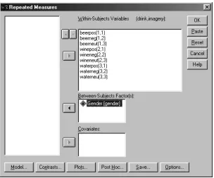
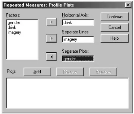
(2) Discovering Statistics Using SPSS: Chapter 12. Figure 1: Completed dialog box for mixed design ANOVA Gender has only two levels (male or female) so there is no need to specify contrasts for this variable; however, you should select simple contrasts for both drink and imagery. The addition of a between-group factor means that we can select post hoc tests for this variable by . This action brings up the post hoc test dialog box, which can be used as clicking on previously explained. However, we need not specify any post hoc tests here because the between-group factor has only two levels. The addition of an extra variable makes it necessary to access the to choose a different graph to the one in the previous example. Click on dialog box in Figure 2. Place drink and imagery in the same slots as for the previous example but also place gender in the slot labelled Separate Plots. When all three variables have been to add this combination to the list of plots. By asking specified, don’t forget to click on SPSS to plot the drink × imagery × gender interaction, we should get the same interaction graph as before, except that a separate version of this graph will be produced for male and female subjects. As far as other options are concerned, you should select the same ones that were chosen in Chapter 11. It is worth selecting estimated marginal means for all effects (because these values will help you to understand any significant effects), but to save space I did not ask for confidence intervals for these effects because we have considered this part of the output in some detail already. When all of the appropriate options have been selected, run the analysis.. Dr. Andy Field. Page 2. 6/8/2004.

(3) Discovering Statistics Using SPSS: Chapter 12. Figure 2: Plots dialog box for a three-way mixed ANOVA Main Analysis The initial output is the same as the two-way ANOVA example: there is a table listing the repeated measures variables from the data editor and the level of each independent variable that they represent. The second table contains descriptive statistics (mean and standard deviation) for each of the nine conditions split according to whether subjects were male or female (see SPSS Output 1). The names in this table are the names I gave the variables in the data editor (therefore, your output may differ slightly). These descriptive statistics are interesting because they show us the pattern of means across all experimental conditions (so, we use these means to produce the graphs of the three-way interaction). We can see that the variability among scores was greatest when beer was used as a product, and that when a corpse image was used the ratings given to the products were negative (as expected) for all conditions except the men in the beer condition. Likewise, ratings of products were very positive when a sexy person was used as the imagery irrespective of the gender of the participant, or the product being advertised.. Dr. Andy Field. Page 3. 6/8/2004.

(4) Discovering Statistics Using SPSS: Chapter 12. Descriptive Statistics Std. Deviation. Gender. Mean. Beer + Sexy. Male Female Total. 24.8000 17.3000 21.0500. 14.0063 11.3925 13.0080. N 10 10 20. Beer + Corpse. Male Female Total. 20.1000 -11.2000 4.4500. 7.8379 5.1381 17.3037. 10 10 20. Beer + Person in Armchair. Male Female Total. 16.9000 3.1000 10.0000. 8.5434 6.7074 10.2956. 10 10 20. Wine + Sexy. Male Female Total. 22.3000 28.4000 25.3500. 7.6311 4.1150 6.7378. 10 10 20. Wine + Corpse. Male Female Total. -7.8000 -16.2000 -12.0000. 4.9396 4.1312 6.1815. 10 10 20. Wine + Person in Armchair. Male Female Total. 7.5000 15.8000 11.6500. 4.9721 4.3919 6.2431. 10 10 20. Water + Sexy. Male Female Total. 14.5000 20.3000 17.4000. 6.7864 6.3953 7.0740. 10 10 20. Water + Corpse. Male Female Total. -9.8000 -8.6000 -9.2000. 6.7791 7.1368 6.8025. 10 10 20. Water + Person in Armchair. Male Female Total. -2.1000 6.8000 2.3500. 6.2973 3.8816 6.8386. 10 10 20. SPSS Output 1 SPSS Output 2 shows the results of Mauchly’s sphericity test for each of the three repeated measures effects in the model. The values of these tests are different to the previous example, because the between-group factor is now being accounted for by the test. The main effect of drink still significantly violates the sphericity assumption (W = 0.572, p < 0.01) but the main effect of imagery no longer does. Therefore, the F value for the main effect of drink (and its interaction with the between-group variable gender) needs to be corrected for this violation. Mauchly's Test of Sphericityb Measure: MEASURE_1. Within Subjects Effect DRINK IMAGERY DRINK * IMAGERY. Mauchly's W .572 .965 .609. Approx. Chi-Square 9.486 .612 8.153. a. df. Sig. 2 2 9. Greenhouse-Geisser. Epsilon Huynh-Feldt. Lower-bound. .700 .966 .813. .784 1.000 1.000. .500 .500 .250. .009 .736 .521. Tests the null hypothesis that the error covariance matrix of the orthonormalized transformed dependent variables is proportional to an identity matrix. a. May be used to adjust the degrees of freedom for the averaged tests of significance. Corrected tests are displayed in the layers (by default) of the Tests of Within Subjects Effects table. b. Design: Intercept+GENDER - Within Subjects Design: DRINK+IMAGERY+DRINK*IMAGERY. SPSS Output 2 SPSS Output 3 shows the summary table of the repeated measures effects in the ANOVA with corrected F values. The output is split into sections for each of the effects in the model and their associated error terms. The table format is the same as for the previous example, except that the interactions between gender and the repeated measures effects are included also. We would expect to still find the affects that were previously present (in a balanced design, the inclusion of an extra variable should not effect these effects). By looking at the significance values it is clear that this prediction is true: there are still significant effects of the type of drink used, the type of imagery used, and the interaction of these two variables.. Dr. Andy Field. Page 4. 6/8/2004.

(5) Discovering Statistics Using SPSS: Chapter 12 In addition to the effects already described we find that gender interacts significantly with the type of drink used (so, men and women respond differently to beer, wine and water regardless of the context of the advert). There is also a significant interaction of gender and imagery (so, men and women respond differently to positive, negative and neutral imagery regardless of the drink being advertised). Finally, the three-way interaction between gender, imagery and drink is significant, indicating that the way in which imagery affects responses to different types of drinks depends on whether the subject is male or female. The effects of the repeated measures variables have been outlined in Chapter 11 and the pattern of these responses will not have changed, so rather than repeat myself, I will concentrate on the new effects and the forgetful reader should look back at Chapter 11! Tests of Within-Subjects Effects Measure: MEASURE_1. Source. Type III Sum of Squares. df. Mean Square. F. Sig.. DRINK. Sphericity Assumed Greenhouse-Geisser Huynh-Feldt Lower-bound. 2092.344 2092.344 2092.344 2092.344. 2 1.401 1.567 1.000. 1046.172 1493.568 1334.881 2092.344. 11.708 11.708 11.708 11.708. .000 .001 .000 .003. DRINK * GENDER. Sphericity Assumed Greenhouse-Geisser Huynh-Feldt Lower-bound. 4569.011 4569.011 4569.011 4569.011. 2 1.401 1.567 1.000. 2284.506 3261.475 2914.954 4569.011. 25.566 25.566 25.566 25.566. .000 .000 .000 .000. Error(DRINK). Sphericity Assumed Greenhouse-Geisser Huynh-Feldt Lower-bound. 3216.867 3216.867 3216.867 3216.867. 36 25.216 28.214 18.000. 89.357 127.571 114.017 178.715. IMAGERY. Sphericity Assumed Greenhouse-Geisser Huynh-Feldt Lower-bound. 21628.678 21628.678 21628.678 21628.678. 2 1.932 2.000 1.000. 10814.339 11196.937 10814.339 21628.678. 287.417 287.417 287.417 287.417. .000 .000 .000 .000. IMAGERY * GENDER. Sphericity Assumed Greenhouse-Geisser Huynh-Feldt Lower-bound. 1998.344 1998.344 1998.344 1998.344. 2 1.932 2.000 1.000. 999.172 1034.522 999.172 1998.344. 26.555 26.555 26.555 26.555. .000 .000 .000 .000. Error(IMAGERY). Sphericity Assumed Greenhouse-Geisser Huynh-Feldt Lower-bound. 1354.533 1354.533 1354.533 1354.533. 36 34.770 36.000 18.000. 37.626 38.957 37.626 75.252. DRINK * IMAGERY. Sphericity Assumed Greenhouse-Geisser Huynh-Feldt Lower-bound. 2624.422 2624.422 2624.422 2624.422. 4 3.251 4.000 1.000. 656.106 807.186 656.106 2624.422. 19.593 19.593 19.593 19.593. .000 .000 .000 .000. DRINK * IMAGERY * GENDER. Sphericity Assumed Greenhouse-Geisser Huynh-Feldt Lower-bound. 495.689 495.689 495.689 495.689. 4 3.251 4.000 1.000. 123.922 152.458 123.922 495.689. 3.701 3.701 3.701 3.701. .009 .014 .009 .070. Error(DRINK*IMAGERY). Sphericity Assumed Greenhouse-Geisser Huynh-Feldt Lower-bound. 2411.000 2411.000 2411.000 2411.000. 72 58.524 72.000 18.000. 33.486 41.197 33.486 133.944. SPSS Output 3 The Effect of Gender The main effect of gender is listed separately from the repeated measure effects in a table labelled Tests of Between-Subjects Effects. Before looking at this table it is important to check the assumption of homogeneity of variance using Levene’s test (see Chapter 3). SPSS produces a table listing Levene’s test for each of the repeated measures variables in the data editor, and we need to look for any variable that has a significant value. SPSS Output 4 shows both tables. The table showing Levene’s test indicates that variances are homogeneous for all levels of the repeated measures variables (because all significance values are greater than 0.05). If any values were significant, then this would compromise the accuracy of the F-test for gender, and we would have to consider transforming all of our data to stabilize the variances between groups (one popular transformation is to take the square root of all values). Fortunately, in this example a transformation is unnecessary. The second table shows the. Dr. Andy Field. Page 5. 6/8/2004.

(6) Discovering Statistics Using SPSS: Chapter 12 ANOVA summary table for the main effect of gender, and this reveals a significant effect (because the significance of 0.018 is less than the standard cut-off point of 0.05). a Levene's Test of Equality of Error Variances. F Beer + Sexy Beer + Corpse Beer + Person in Armchair Wine + Sexy Wine + Corpse Wine + Person in Armchair Water + Sexy Water + Corpse Water + Person in Armchair. df1. 1.009 1.305 1.813 2.017 1.048 .071 .317 .804 1.813. df2 1 1 1 1 1 1 1 1 1. Sig. 18 18 18 18 18 18 18 18 18. .328 .268 .195 .173 .320 .793 .580 .382 .195. Tests the null hypothesis that the error variance of the dependent variable is equal across groups. a. Design: Intercept+GENDER - Within Subjects Design: DRINK+IMAGERY+DRINK*IMAGERY. Tests of Between-Subjects Effects Measure: MEASURE_1 Transformed Variable: Average. Source. Type III Sum of Squares. Intercept GENDER Error. 1246.445 58.178 155.167. Mean Square. df 1 1 18. 1246.445 58.178 8.620. F 144.593 6.749. Sig. .000 .018. SPSS Output 4 We can report that there was a significant main effect of gender (F(1, 18) = 6.75, p < 0.05). This effect tells us that if we ignore all other variables, male subjects’ ratings were significantly different to females. If you requested that SPSS display means for the gender effect you should scan through your output and find the table in a section headed Estimated Marginal Means. SPSS Output 5 is a table of means for the main effect of gender with the associated standard errors. This information is plotted in Figure 3. It is clear from this graph that men’s ratings were generally significantly more positive than females. Therefore, men gave more positive ratings than women regardless of the drink being advertised and the type of imagery used in the advert. 15.00 9.60. Estimates. 10.00. Measure: MEASURE_1. Gender Male Female. Mean 9.600 6.189. Std. Error .928 .928. 95% Confidence Interval Lower Upper Bound Bound 7.649 4.238. 6.19. 5.00. 11.551 8.140. 0.00 Male. Female. Figure 3. SPSS Output 5 The Interaction between Gender and Drink. SPSS Output 3 indicated that gender interacted in some way with the type of drink used as a stimulus. Remembering that the effect of drink violated sphericity, we must report Greenhouse-Geisser corrected values for this interaction with the between-group factor. From the summary table we should report that there was a significant interaction between the type of drink used and the gender of the subject (F(1.40, 25.22) = 25.57, p < 0.001). This effect tells us that the type of drink being advertised had a different effect on men and women. We can use the estimated marginal means to determine the nature of this interaction (or we could. Dr. Andy Field. Page 6. 6/8/2004.

(7) Discovering Statistics Using SPSS: Chapter 12 have asked SPSS for a plot of gender × drink using the dialog box in Figure 2). The means and interaction graph (Figure 4 and SPSS Output 6) show the meaning of this result. The graph shows the average male ratings of each drink ignoring the type of imagery with which it was presented (circles). The women’s scores are shown as squares. The graph clearly shows that male and female ratings are very similar for wine and water, but men seem to rate beer more highly than women—regardless of the type of imagery used. We could interpret this interaction as meaning that the type of drink being advertised influenced ratings differently in men and women. Specifically, ratings were similar for wine and water but males rated beer higher than women. This interaction can be clarified using the contrasts specified before the analysis. 2. Gender * DRINK. 25. Measure: MEASURE_1. Mean. Std. Error. 20. 95% Confidence Interval Lower Upper Bound Bound. 15. Gender. DRINK. Male. 1 2 3. 20.600 7.333 .867. 2.441 .765 1.414. 15.471 5.726 -2.103. 25.729 8.940 3.836. 10. Female. 1 2 3. 3.067 9.333 6.167. 2.441 .765 1.414. -2.062 7.726 3.197. 8.196 10.940 9.136. 0. 5. Beer. SPSS Output 6. Wine. Water. Figure 4. The Interaction between Gender and Imagery SPSS Output 3 indicated that gender interacted in some way with the type of imagery used as a stimulus. The effect of imagery did not violate sphericity, so we can report the uncorrected F value. From the summary table we should report that there was a significant interaction between the type of imagery used and the gender of the subject (F(2, 36) = 26.55, p < 0.001). This effect tells us that the type of imagery used in the advert had a different effect on men and women. We can use the estimated marginal means to determine the nature of this interaction (or we could have asked SPSS for a plot of imagery × gender using the dialog box in Figure 2). The means and interaction graph (Figure 5 and SPSS Output 7) show the meaning of this result. The graph shows the average male in each imagery condition ignoring the type of drink that was rated (circles). The women’s scores are shown as squares. The graph clearly shows that male and female ratings are very similar for positive and neutral imagery, but men seem to be less affected by negative imagery than women—regardless of the drink in the advert. To interpret this finding more fully, we should consult the contrasts for this interaction. 30. 3. Gender * IMAGERY Measure: MEASURE_1. Mean. Std. Error. Gender. IMAGERY. Male. 1 2 3. 20.533 .833 7.433. 1.399 1.092 1.395. 17.595 -1.460 4.502. 23.471 3.127 10.365. Female. 1 2 3. 22.000 -12.000 8.567. 1.399 1.092 1.395. 19.062 -14.293 5.635. 24.938 -9.707 11.498. SPSS Output 7. 20. 95% Confidence Interval Lower Upper Bound Bound. 10 0 -10. Pos. Neg. Neut. -20. Figure 5. The Interaction between Drink and Imagery The interpretation of this interaction is the same as for the two-way ANOVA (see Chapter 11). You may remember that the interaction reflected the fact that negative imagery has a different effect to both positive and neutral imagery (because it decreased ratings rather than increasing them).. Dr. Andy Field. Page 7. 6/8/2004.

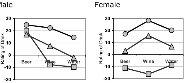
(8) Discovering Statistics Using SPSS: Chapter 12 The Interaction between Gender, Drink and Imagery The three-way interaction tells us whether the drink by imagery interaction is the same for men and women (i.e. whether the combined effect of the type of drink and the imagery used is the same for male subjects as for female subjects). We can conclude that there is a significant three-way drink × imagery × gender interaction (F(4, 72) = 3.70, p < 0.01). The nature of this interaction is shown up in Figure 6, which shows the imagery by drink interaction for men and women separately. The male graph shows that when positive imagery is used, men generally rated all three drinks positively (the line with circles is higher than the other lines for all drinks). This pattern is true of women also (the line representing positive imagery is above the other two lines). When neutral imagery is used, men rate beer very highly, but rate wine and water fairly neutrally. Women, on the other hand rate beer and water neutrally, but rate wine more positively (in fact, the pattern of the positive and neutral imagery lines show that women generally rate wine slightly more positively than water and beer). So, for neutral imagery men still rate beer positively, and women still rate wine positively. For the negative imagery, the men still rate beer very highly, but give low ratings to the other two types of drink. So, regardless of the type of imagery used, men rate beer very positively (if you look at the graph you’ll note that ratings for beer are virtually identical for the three types of imagery). Women, however, rate all three drinks very negatively when negative imagery is used. The three-way interaction is, therefore, likely to reflect these sex differences in the interaction between drink and imagery. Specifically, men seem fairly immune to the effects of imagery when beer is being used as a stimulus, whereas women are not. The contrasts will show up exactly what this interaction represents. 4. Gender * DRINK * IMAGERY Measure: MEASURE_1. Gender. DRINK. IMAGERY. Male. 1. 1 2 3. 24.800 20.100 16.900. 4.037 2.096 2.429. 16.318 15.697 11.797. 33.282 24.503 22.003. 2. 1 2 3. 22.300 -7.800 7.500. 1.939 1.440 1.483. 18.227 -10.825 4.383. 26.373 -4.775 10.617. 3. 1 2 3. 14.500 -9.800 -2.100. 2.085 2.201 1.654. 10.119 -14.424 -5.575. 18.881 -5.176 1.375. 1. 1 2 3. 17.300 -11.200 3.100. 4.037 2.096 2.429. 8.818 -15.603 -2.003. 25.782 -6.797 8.203. 2. 1 2 3. 28.400 -16.200 15.800. 1.939 1.440 1.483. 24.327 -19.225 12.683. 32.473 -13.175 18.917. 3. 1 2 3. 20.300 -8.600 6.800. 2.085 2.201 1.654. 15.919 -13.224 3.325. 24.681 -3.976 10.275. Female. Mean. Std. Error. 95% Confidence Interval Lower Upper Bound Bound. SPSS Output 8. Dr. Andy Field. Page 8. 6/8/2004.

(9) Discovering Statistics Using SPSS: Chapter 12. Female. 30. 30. 20. 20. 10 0 Beer. Wine. Water. Rating of Drink. Rating of Drink. Male. 10 0 Beer. -10. -10. -20. -20. Wine. Water. Figure 6: Graphs showing the drink by imagery interaction for men and women. Lines represent positive imagery (circles), negative imagery (squares) and neutral imagery (triangles) Contrasts for Repeated Measures Variables We requested simple contrasts for the drink variable (for which water was used as the control category) and for the imagery category (for which neutral imagery was used as the control category). SPSS Output 9 shows the summary results for these contrasts. The table is the same as for the previous example except that the added effects of gender and its interaction with other variables are now included. So, for the main effect of drink, the first contrast compares level 1 (beer) against the base category (in this case, the last category: water). This result is significant (F(1, 18) = 15.37, p < 0.01), and the next contrast compares level 2 (wine) with the base category (water) and confirms the significant difference found when gender was not included as a variable in the analysis (F(1, 18) = 19.92, p < 0.001). For the imagery main effect, the first contrast compares level 1 (positive) to the base category (neutral) and verifies the significant effect found by the post hoc tests (F(1, 18) = 134.87, p < 0.001). The second contrast confirms the significant difference found for the negative imagery condition compared to the neutral (F(1, 18) = 129.18, p < 0.001). No contrast was specified for gender. Tests of Within-Subjects Contrasts Measure: MEASURE_1 Mean Square. DRINK. DRINK. Level 1 vs. Level 3. 1383.339. 1. 1383.339. 15.371. .001. Level 2 vs. Level 3. 464.006. 1. 464.006. 19.923. .000. Level 1 vs. Level 3. 2606.806. 1. 2606.806. 28.965. .000. Level 2 vs. Level 3. 54.450. 1. 54.450. 2.338. .144. Level 1 vs. Level 3. 1619.967. 18. 89.998. DRINK * GENDER Error(DRINK). IMAGERY. Type III Sum of Squares. Source. Level 2 vs. Level 3. df. F. Sig.. 419.211. 18. 23.290. IMAGERY. Level 1 vs. Level 3 Level 2 vs. Level 3. 3520.089 3690.139. 1 1. 3520.089 3690.139. 134.869 129.179. .000 .000. IMAGERY * GENDER. Level 1 vs. Level 3 Level 2 vs. Level 3. .556 975.339. 1 1. .556 975.339. .021 34.143. .886 .000. Error(IMAGERY). Level 1 vs. Level 3 Level 2 vs. Level 3. 469.800. 18. 26.100. 514.189. 18. 28.566. Level 1 vs. Level 3. Level 1 vs. Level 3 Level 2 vs. Level 3. 320.000 720.000. 1 1. 320.000 720.000. 1.686 8.384. .211 .010. Level 2 vs. Level 3. Level 1 vs. Level 3 Level 2 vs. Level 3. 36.450. 1. 36.450. .223. .642. 2928.200. 1. 2928.200. 31.698. .000. Level 1 vs. Level 3. Level 1 vs. Level 3 Level 2 vs. Level 3. 441.800 480.200. 1 1. 441.800 480.200. 2.328 5.592. .144 .029. Level 2 vs. Level 3. Level 1 vs. Level 3 Level 2 vs. Level 3. 4.050 405.000. 1 1. 4.050 405.000. .025 4.384. .877 .051. Level 1 vs. Level 3. Level 1 vs. Level 3 Level 2 vs. Level 3. 3416.200 3416.200. 18 18. 189.789 189.789. Level 2 vs. Level 3. Level 1 vs. Level 3 Level 2 vs. Level 3. 1545.800 1662.800. 18 18. 85.878 92.378. DRINK * IMAGERY. DRINK * IMAGERY * GENDER. Error(DRINK*IMAGERY). SPSS Output 9. Dr. Andy Field. Page 9. 6/8/2004.

(10) Discovering Statistics Using SPSS: Chapter 12 Drink × Gender Interaction 1: Beer vs. Water, Male vs. Female The first interaction term looks at level 1 of drink (beer) compared to level 3 (water), comparing male and female scores. This contrast is highly significant (F(1, 18) = 28.97, p < 0.001). This result tells us that the increased ratings of beer compared to water found for men are not found for women. So, in Figure 4 the squares representing female ratings of beer and water are roughly level; however, the circle representing male ratings of beer is much higher than the circle representing water. The positive contrast represents this difference and so we can conclude that male ratings of beer (compared to water) were significantly greater than women’s ratings of beer (compared to water). Drink × Gender Interaction 2: Wine vs. Water, Male vs. Female The second interaction term compares level 2 of drink (wine) to level 3 (water), contrasting male and female scores. There is no significant difference for this contrast (F(1, 18) = 2.34, p = 0.14), which tells us that the difference between ratings of wine compared to water in males is roughly the same as in females. Therefore, overall, the drink × gender interaction has shown up a difference between males and females in how they rate beer (regardless of the type of imagery used). Imagery × Gender Interaction 1: Positive vs. Neutral, Male vs. Female The first interaction term looks at level 1 of imagery (positive) compared to level 3 (neutral), comparing male and female scores. This contrast is not significant (F < 1). This result tells us that ratings of drinks presented with positive imagery (relative to those presented with neutral imagery) were equivalent for males and females. This finding represents the fact that in Figure 5 the squares and circles for both the positive and neutral conditions overlap (therefore male and female responses were the same. Imagery × Gender Interaction 2: Negative vs. Neutral, Male vs. Female The second interaction term looks at level 2 of imagery (negative) compared to level 3 (neutral), comparing male and female scores. This contrast is highly significant (F(1, 18) = 34.13, p < 0.001). This result tells us that the difference between ratings of drinks paired with negative imagery compared to neutral was different for men and women. Looking at Figure 5 this finding represents the fact that for men, ratings of drinks paired with negative imagery were relatively similar to ratings of drinks paired with neutral imagery (the circles have a fairly similar vertical position). However, if you look at the female ratings, then drinks were rated much less favourably when presented with negative imagery than when presented with neutral imagery (the square in the negative condition is much lower than the neutral condition). Therefore, overall, the imagery × gender interaction has shown up a difference between males and females in terms of their ratings to drinks presented with negative imagery compared to neutral; specifically, men seem less affected by negative imagery. Drink × Imagery × Gender Interaction 1: Beer vs. Water, Positive vs. Neutral Imagery, Male vs. Female The first interaction term compares level 1 of drink (beer) to level 3 (water), when positive imagery (level 1) is used compared to neutral (level 3) in males compared to females (F(1, 18) = 2.33, p = 0.144). The non-significance of this contrast tells us that the difference in ratings when positive imagery is used compared to neutral imagery is roughly equal when beer is used as a stimulus as when water is used, and these differences are equivalent in male and female subjects. In terms of the interaction graph (Figure 6) it means that the distance between the circle and the triangle in the beer condition is the same as the distance between the circle and the triangle in the water condition and that these distances are equivalent in men and women. Drink × Imagery × Gender Interaction 2: Beer vs. Water, Negative vs. Neutral Imagery, Male vs. Female. Dr. Andy Field. Page 10. 6/8/2004.

(11) Discovering Statistics Using SPSS: Chapter 12 The second interaction term looks at level 1 of drink (beer) compared to level 3 (water), when negative imagery (level 2) is used compared to neutral (level 3). This contrast is significant (F(1, 18) = 5.59, p < 0.05). This result tells us that the difference in ratings between beer and water when negative imagery is used (compared to neutral imagery) is different between men and women. If we plot ratings of beer and water across the negative and neutral conditions, for males 30 (circles) and females (squares) separately, we see Wate Beer that ratings after negative imagery are always lower 20 than ratings for neutral imagery except for men’s ratings of beer, which are actually higher after 10 negative imagery. As such, this contrast tells us that 0 the interaction effect reflects a difference in the way Negative Neutral Negative Neutral in which males rate beer compared to females when -10 negative imagery is used compared to neutral. Males and females are similar in their pattern of ratings for -20 water but different in the way in which they rate beer. Drink × Imagery × Gender Interaction 3: Wine vs. Water, Positive vs. Neutral Imagery, Male vs. Female. The third interaction term looks at level 2 of drink (wine) compared to level 3 (water), when positive imagery (level 1) is used compared to neutral (level 3) in males compared to females. This contrast is non-significant (F (1, 18) < 1). This result tells us that the difference in ratings when positive imagery is used compared to neutral imagery is roughly equal when wine is used as a stimulus as when water is used, and these differences are equivalent in male and female subjects. In terms of the interaction graph (Figure 6) it means that the distance between the circle and the triangle in the wine condition is the same as the distance between the circle and the triangle in the water condition and that these distances are equivalent in men and women. Drink × Imagery × Gender Interaction 4: Wine vs. Water, Negative vs. Neutral Imagery, Male vs. Female. The final interaction term looks at level 2 of drink (wine) compared to level 3 (water), when negative imagery (level 2) is used compared to neutral (level 3). This contrast is very close to significance (F(1, 18) = 4.38, p = 0.051). This result tells us that the difference in ratings between wine 30 and water when negative imagery is used (compared to neutral imagery) is different between men and 20 Wine Wate women (although this difference has not quite reached significance). If we plot ratings of wine and 10 water across the negative and neutral conditions, for 0 males (circles) and females (squares), we see that Negative Neutral Negative Neutral ratings after negative imagery are always lower than -10 ratings for neutral imagery, but for women rating wine the change is much more dramatic (the line is -20 steeper). As such, this contrast tells us that the interaction effect reflects a difference in the way in which females rate wine differently to males when neutral imagery is used compared to when negative imagery is used. Males and females are similar in their pattern of ratings for water but different in the way in which they rate wine. It is noteworthy that this contrast was not significant using the usual 0.05 level; however, it is worth remembering that this cut-off point was set in a fairly arbitrary way, and so it is worth reporting these close effects and letting your reader decide whether they are meaningful or not. There is also a growing trend towards reporting effect sizes in preference to using significance levels.. Dr. Andy Field. Page 11. 6/8/2004.

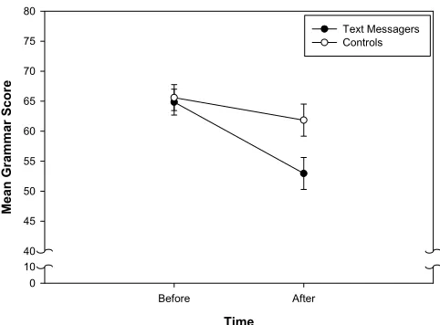
(12) Discovering Statistics Using SPSS: Chapter 12 Summary These contrasts again tell us nothing about the differences between the beer and wine conditions (or the positive and negative conditions) and different contrasts would have to be run to find out more. However, what is clear so far is that differences exist between men and women in terms of their ratings towards beer and wine. It seems as though men are relatively unaffected by negative imagery when it comes to beer. Likewise, women seem more willing to rate wine positively when neutral imagery is used than men do. What should be clear from this is that complex ANOVA in which several independent variables are used results in complex interaction effects that require a great deal of concentration to interpret (imagine interpreting a four-way interaction!). Therefore, it is essential to take a systematic approach to interpretation and plotting graphs is a particularly useful way to proceed. It is also advisable to think carefully about the appropriate contrasts to use to answer the questions you have about your data. It is these contrasts that will help you to interpret interactions, so make sure you select sensible ones!. Task 2 Text messaging is very popular amongst mobile phone owners, to the point that books have been published on how to write in text speak (BTW, hope u kno wat I mean by txt spk). One concern is that children may use this form of communication so much that it will hinder their ability to learn correct written English. One concerned researcher conducted an experiment in which one group of children were encouraged to send text messages on their mobile phones over a six month period. A second group was forbidden from sending text messages for the same period. To ensure that kids in this later group didn’t use their phones, this group were given armbands that administered painful shocks in the presence of microwaves (like those emitted from phones)2. There were 50 different participants: 25 were encouraged to send text messages, and 25 were forbidden. The outcome was a score on a grammatical test (as a percentage) that was measured both before and after the experiment. The first independent variable was, therefore, text message use (text messagers versus controls) and the second independent variable was the time at which grammatical ability was assessed (before or after the experiment). The data are in the file TextMessages.sav. SPSS Output Figure 7 shows a line chart (with error bars) of the grammar data. The dots show the mean grammar score before and after the experiment for the text message group and the controls. The means before and after are connected by a line for the two groups separately. It’s clear from this chart that in the text message group grammar scores went down dramatically over the 6 month period in which they used their mobile phone. For the controls, their grammar scores also fell but much less dramatically.. 2 Although this punished them for any attempts to use a mobile phone, an unfortunate side effect was that 10 of the sample developed conditioned phobias of porridge after repeatedly trying to heat some up in the microwave!. Dr. Andy Field. Page 12. 6/8/2004.

(13) Discovering Statistics Using SPSS: Chapter 12. 80 Text Messagers Controls. 75. Mean Grammar Score. 70 65 60 55 50 45 40 10 0 Before. After. Time. Figure 7: Line chart (with error bars showing the standard error of the mean) of the mean grammar scores before and after the experiment for text messagers and controls Descriptive Statistics Grammer at Time 1. Grammar at Time 2. Group Text Messagers Controls Total Text Messagers Controls Total. Mean 64.8400 65.6000 65.2200 52.9600 61.8400 57.4000. Std. Deviation 10.67973 10.83590 10.65467 16.33116 9.41046 13.93278. N 25 25 50 25 25 50. The output above shows the table of descriptive statistics from the two-way mixed ANOVA; the table has means at time one split according to whether the people were in the text messaging group or the control group, then below we have the means for the two groups at time 2. These means correspond to those plotted in Figure 7. Mauchly's Test of Sphericityb Measure: MEASURE_1 Epsilon Within Subjects Effect TIME. Mauchly's W 1.000. Approx. Chi-Square .000. df. Sig. 0. .. GreenhouseGeisser 1.000. a. Huynh-Feldt 1.000. Lower-bound 1.000. Tests the null hypothesis that the error covariance matrix of the orthonormalized transformed dependent variables is proportional to an identity matrix. a. May be used to adjust the degrees of freedom for the averaged tests of significance. Corrected tests are displayed in the Tests of Within-Subjects Effects table. b. Design: Intercept+GROUP Within Subjects Design: TIME. a Levene's Test of Equality of Error Variances. Grammer at Time 1 Grammar at Time 2. F .089 3.458. df1. df2 1 1. 48 48. Sig. .767 .069. Tests the null hypothesis that the error variance of the dependent variable is equal across groups. a. Design: Intercept+GROUP Within Subjects Design: TIME. We know that when we use repeated measures we have to check the assumption of sphericity. We also know that for independent designs we need to check the homogeneity of variance assumption. If the design is a mixed design then we have both repeated and independent measures, so we have to check both assumptions. In this case, we have only two levels of the repeated measure so the assumption of sphericity does not apply in this case. Levene’s test, produces a different test for each level of the repeated measures variable. In mixed designs,. Dr. Andy Field. Page 13. 6/8/2004.

(14) Discovering Statistics Using SPSS: Chapter 12 the homogeneity assumption has to hold for every level of the repeated measures variable. At both levels of time, Levene’s test is nonsignificant (p = 0.77 before the experiment and p = 0.069 after the experiment). This means the assumption has not been broken at all (but it was quite close to being a problem after the experiment). Tests of Within-Subjects Effects Measure: MEASURE_1 Source TIME. TIME * GROUP. Error(TIME). Sphericity Assumed Greenhouse-Geisser Huynh-Feldt Lower-bound Sphericity Assumed Greenhouse-Geisser Huynh-Feldt Lower-bound Sphericity Assumed Greenhouse-Geisser Huynh-Feldt Lower-bound. Type III Sum of Squares 1528.810 1528.810 1528.810 1528.810 412.090 412.090 412.090 412.090 4747.600 4747.600 4747.600 4747.600. df 1 1.000 1.000 1.000 1 1.000 1.000 1.000 48 48.000 48.000 48.000. Mean Square 1528.810 1528.810 1528.810 1528.810 412.090 412.090 412.090 412.090 98.908 98.908 98.908 98.908. F 15.457 15.457 15.457 15.457 4.166 4.166 4.166 4.166. Sig. .000 .000 .000 .000 .047 .047 .047 .047. Tests of Between-Subjects Effects Measure: MEASURE_1 Transformed Variable: Average Source Intercept GROUP Error. Type III Sum of Squares 375891.610 580.810 9334.080. df 1 1 48. Mean Square 375891.610 580.810 194.460. F 1933.002 2.987. Sig. .000 .090. The output above shows the main ANOVA summary tables. Like any two-way ANOVA, we still have three effects to find: two main effects (one for each independent variable) and one interaction term. The main effect of time is significant so we can conclude that grammar scores were significantly affected by the time at which they were measured. The exact nature of this effect is easily determined because there were only two points in time (and so this main effect is comparing only two means). The graph shows that grammar scores were higher before the experiment than after. So, before the experimental manipulation scores were higher than after, meaning that the manipulation had the net effect of significantly reducing grammar scores. This main effect seems rather interesting until you consider that these Group means include both text messagers and controls. There are three possible reasons for the drop in grammar scores: (1) the text messagers got worse and are dragging down the mean after the experiment, (2) the controls somehow got worse, or (3) the whole group just got worse and it had nothing to do with whether the children text messaged or not. Until we examine the interaction, we won’t see which of these is true. Mean Grammar Score (%). 70. 60. 50. 40 10. 0. Before. After. The main effect of group is shown by the F-ratio in the second table above. The probability associated with this F-ratio is 0.09, which is just above the critical value of 0.05. Therefore, we must conclude that there was no significant main effect on grammar scores of whether children text-messaged or not. Again, this effect seems interesting enough and mobile phone companies might certainly chose to cite it as evidence that text messaging does not affect your grammar ability. However, remember that this main effect ignores the time at which grammar ability is measured. It just means that if we took the average grammar score for text messagers (that’s including their score both before and after they started Group using their phone), and compared this to the mean of the controls (again including scores before and after) then these means would not be significantly Mean Grammar Score (%). 70. 60. 50. 40 10. 0. Text Messagers. Dr. Andy Field. Page 14. Controls. 6/8/2004.

(15) Discovering Statistics Using SPSS: Chapter 12 different. The graph shows that when you ignore the time at which grammar was measured, the controls have slightly better grammar than the text messagers—but not significantly so. Main effects are not always that interesting and should certainly be viewed in the context of any interaction effects. The interaction effect in this example is shown by the F-ratio in the row labeled Time*Group, and because the probability of obtaining a value this big by chance is 0.047, which is just less than the criterion of 0.05, we can say that there is a significant interaction between the time at which grammar was measured and whether or not children were allowed to text message within that time. The mean ratings in all conditions (see Figure 7) help us to interpret this effect. The significant interaction tells us that the change in grammar scores was significantly different in text messagers compared to controls. Looking at Figure 7 we can see that although grammar scores fell in controls, the drop was much more marked in the text messagers; so, text messaging does seem to ruin your ability at grammar compared to controls3. Writing the Result We can report the three effects from this analysis as follows: •. The results show that the grammar ratings at the end of the experiment were significantly lower than those at the beginning of the experiment, F(1, 48) = 15.46, p < .001, r = .61.. •. The main effect of group on the grammar scores was nonsignificant, F(1, 48) = 2.99, ns, r = .27. This indicated that when the time at which grammar was measured is ignored, the grammar ability in the text message group was not significantly different to the controls.. •. The time × group interaction was significant, F(1, 48) = 4.17, p < .05, r = .34, indicating that the change in grammar ability in the text message group was significantly different to the change in the control groups. These findings indicate that although there was a natural decay of grammatical ability over time (as shown by the controls) there was a much stronger effect when participants were encouraged to use text messages. This shows that using text messages accelerates the inevitable decline in grammatical ability.. 3. It’s interesting that the control group means dropped too. This could be because the control group were undisciplined and still used their mobile phones, or it could just be that the education system in this country is so under funded that there is no-one to teach English anymore!. Dr. Andy Field. Page 15. 6/8/2004.

(16)

No results found