Exponential-time differencing schemes for low-mass DPD systems

Exponential-time differencing schemes for low-mass DPD

systems

N. Phan-Thien

, N. Mai-Duy

, D. Pan

and B. C. Khoo

,

1

_{Department of Mechanical Engineering, Faculty of Engineering,}

National University of Singapore, Singapore.

2

_{Computational Engineering and Science Research Centre,}

Faculty of Engineering and Surveying,

University of Southern Queensland, Toowoomba, QLD 4350, Australia.

Submitted to

Computer Physics Communications

, August 2012; revised, August

2013

Abstract

Several exponential-time differencing (ETD) schemes are introduced into the method of dissipative

particle dynamics (DPD) to solve the resulting stiff stochastic differential equations in the limit of

small mass, where emphasis is placed on the handling of the fluctuating terms (i.e.,those involving

the random forces). Their performances are investigated numerically in some test viscometric flows.

Results obtained show that the present schemes outperform the velocity-Verlet algorithm regarding

both the satisfaction of equipartition and the maximum allowable time step.

Keywords: exponential-time differencing scheme, dissipative particle dynamics, stiff stochastic

differential equation, overdamped systems

1

Introduction

The DPD method has emerged as a powerful computational tool for predicting hydrodynamic

behaviour of complex-structure fluids like polymers and colloidal suspensions [1-9]. In the DPD

method, a fluid is modelled by a set of particles that can move freely and the system conserves

both mass and momentum. The stochastic differential equations governing the motion of a particle

are given by

dri

dt =vi, (1)

mi

dvi

dt =Fi, (2)

where mi, ri and vi represent the mass, position and velocity vector of a particle i, respectively;

and Fi is the total force vector exerted on it, containing three parts

Fi = N

X

j=1,j6=i

(Fij,C +Fij,D +Fij,R), (3)

in which the sum runs over all other particles, denoted byj, within a certain cutoff radiusrc. The

first term on the right is referred to as the conservative force (subscriptC), the second dissipative

the forms

Fij,C =aijwCeij, (4)

Fij,D =−γwD(eij ·vij)eij, (5)

Fij,R=σwRθijeij, (6)

where aij, γ and σ are constants reflecting the strengths of these forces; wC, wD and wR the

distance-dependent weighting functions; eij = rij/rij a unit vector from particle j to particle i

(rij =ri−rj,rij =|rij|);vij =vi−vj the relative velocity vector, and θij a Gaussian white noise

(θij =θji) with stochastic properties

hθiji= 0, (7)

hθij(t)θkl(t′)i= (δikδjl+δilδjk)δ(t−t′),with i6=k and j 6=l. (8)

It was shown [3] that the equilibrium and detailed balance of the system lead to the following

constraints

wD(rij) = (wR(rij))2, (9)

kBT =

σ2

2γ, (10)

which relate the strength of the dissipative force to the strength of the random force through the

definition of the thermodynamic temperature (the equipartition principle or fluctuation-dissipation

theorem). A popular choice of the weighting functions is [4,5]

wC(rij) = 1−

rij

rc

, (11)

wD(rij) =

1₋ rij

rc

s

. (12)

wheres is a constant (s= 2 ands= 1/2 are two typical values of s).

A considerable effort has been put into the development of numerical integration schemes to

ad-vance particles positions and velocities. Examples of integrators include the Euler-type,

of the fluctuating part are all based on the Wiener process (Brownian motion),i.e.,

∆vi =

1

mi

X

aijwC∆teij −

1

mi

X

γwD(eij ·vij) ∆teij +

1

mi

X

σwR∆Wijeij, (13)

with the autocorrelation defined as

h∆Wij(∆t)∆Wkl(∆t)i =

Z ∆t

0

dt′

Z ∆t

0

dt′′

hθij(t′)θkl(t′′)i

= (δikδjl+δilδjk) ∆t. (14)

This leads to ∆Wij = ξij

√

∆t, where ξij is a random tensor with zero mean and unit variance,

chosen independently for each pair of particles and each time step in the numerical integration

process.

It should be noted that a DPD fluid is compressible in nature [12]. Reducing the mass of the

particles is helpful in many cases - it reduces the Reynolds number, promotes incompressibility via

an increase in the kinematic viscosity and speed of sound, and enhances the dynamic response of

the fluid through an increase in the Schmidt number [13,14]. However, in the limit m _→ 0, the

corresponding DPD systems become stiff (this limit is also called the overdamped limit [15]). It

can be seen that conventional explicit schemes are not efficient to solve such systems as the time

step is limited by the stiff term. In this work, we introduce exponential-time differencing (ETD)

integrators [16] into the DPD model. The stiff term in the deterministic part is treated in an exact

manner, while the fluctuating part is handled according to the Ornstein-Uhlenbeck (O-U) process

[17], which has a bounded variance. These schemes have the ability to handle very different time

scales involved in an effective manner and deliver a convergent solution at large time steps. The

paper is organised as follows. In Section 2, first-order and second-order stochastic ETD schemes

for low mass DPD systems are presented. A modified version of the first-order stochastic ETD is

also included. The verification is conducted by considering some geometric Brownian motions and

2

Proposed integration schemes

Assuming a non-zero mass, the DPD velocity vector equation (2) can be rewritten as

dvi

dt =

1

mi

aijwCeij −

1

mi

γwD(eij ·vij)eij +

1

mi

σwRθijeij. (15)

For brevity, we express a component of the above vector equation in the form

du(t)

dt +cu(t) = a+bθ(t), (16)

where

u= (vi)_α, (17)

c= 1

mi

X

j6=i

γwD

(ri)_α−(rj)_α

rij

2

, (18)

a=₋ 1

mi

3

X

β=1,β6=α

X

j6=i

γwD

(ri)_β −(rj)_β

rij

!

(ri)α−(rj)_α

rij

(vi)_β

+ 1

mi

X

j6=i

γwD(eij ·vj)

_(r

i)_α−(rj)_α

rij

+ 1

mi

X

j6=i

aijwC

_(r

i)_α−(rj)_α

rij

, (19)

b = 1

mi

X

j6=i

σwR

(ri)α−(rj)_α

rij

, (20)

in which the subscript α, β(= 1,2,3) is used to denote the αth component of the vectors in

parentheses. It is noted that Groot and Warren [5] reported the following approximation for the

stiff parameter

c= 1

3τ, (21)

where

1

τ =γ

X

j6=i

wij,Deij.eij ≈4πγn

Z ∞

0

r2wD(r)dr. (22)

In many cases, the mass of the system (c−1_{) goes to zero resulting in a stiff stochastic differential}

equation. It is of our interest to investigate numerical means to integrate (16).

t_→t+ ∆t

ec(t+∆t)_{u(t+ ∆t) =e}ct_{u(t) +e}ct

Z ∆t

0

ecτ_{(a(t+τ) +b(t+τ)θ(t+τ))dτ,}

to yield the displacement u(t+ ∆t) at the next time step t+ ∆t,

u(t+ ∆t) = e−c∆t_{u(t) + ∆A+ ∆B, (23)}

where

∆A(t; ∆t) = e−c∆t

Z ∆t

0

ecτa(t+τ)dτ, (24)

is the forcing function, and

∆B(t; ∆t) =e−c∆t

Z ∆t

0

ecτ_{b(t+τ)θ(t+τ)dτ, (25)}

is an O-U process. Different integration schemes result from different ways that the integrands in

(24)-(25) are approximated.

2.1

First-Order SETD Scheme

First we explore the treatment in which a = a(t) and b = b(t) are regarded as constants in the

interval (t, t+ ∆t). In this case

∆A= ∆A1(t; ∆t) =e−c∆t

Z ∆t

0

ecτ_{a(t+τ)dτ =} a(t)

c 1−e

−c∆t

, (26)

and

∆B(t; ∆t) = e−c∆t_b(t)

Z ∆t

0

ecτ_θ(t+τ)dτ

= b(t) ∆W1, (27)

where ∆W1 is the O-U process,

∆W1(∆t) =e−c∆t

Z ∆t

0

with zero mean,

h∆W1(∆t)i= 0, (29)

and auto-correlation function

h∆W1(∆t) ∆W1(∆t)i = e−2c∆t

Z ∆t

0

dt′

Z ∆t

0

dt′′ect′

hθ(t+t′)θ(t+t′′)_iect′′

= 1

2c 1−e

−2c∆t

. (30)

We call the resulting scheme (23), with (26) and (27) the first-order stochastic exponential time

differencing (1st SETD) scheme. In summary, the scheme is defined as

u(t+ ∆t) = e−c∆t_{u(t) + ∆A}

1(t; ∆t) +b(t) ∆W1(∆t), (31)

The O-U process ∆W1 =

p

(1₋e−2c∆t_{)/2cξ can be written in terms of a Gaussian distributed}

process ξ with zero mean and unit mean square as indicated.

2.2

Second-Order SETD Scheme

We next explore a scheme whereby a and b are approximated as linear functions in the interval

0< τ <∆t:

a(t+τ) =a(t) + τ

∆t(a(t)−a(t−∆t)) =a(t) +

∆a

∆tτ,

b(t+τ) = b(t) + τ

∆t(b(t)−b(t−∆t)) =b(t) +

∆b

∆tτ,

where ∆a =a(t)₋a(t₋∆t) and ∆b=b(t)₋b(t₋∆t) are the first-order backward differences

for a and b. Then, from (24)

∆A(t; ∆t) = e−c∆t

Z ∆t

0

ecτ_a(t+τ)dτ

= a(t)

c 1−e

−c∆t

+ ∆a ∆te

−c∆t

Z ∆t

0

ecτ_{τ dτ}

= ∆A1(t; ∆t) +

c∆t₋1 +e−c∆t

c2

∆a

∆t

where ∆A1(t; ∆t) has been defined in (26) and

∆A2(t; ∆t) =

c∆t₋1 +e−c∆t

c2

∆a

∆t. (33)

In addition ∆B(t; ∆t) can be integrated as

∆B(t; ∆t) = e−c∆t

Z ∆t

0

ecτ_{b(t+τ)θ(t+τ)dτ}

= b(t) ∆W1+

∆b

∆te

−c∆t

Z ∆t

0

τ ecτ_θ(t+τ)dτ

= b(t) ∆W1+

∆b

∆t∆W2, (34)

where the O-U process ∆W1 has been defined in (28), and the O-U process ∆W2 is defined as

∆W2(∆t) =e−c∆t

Z ∆t

0

τ ecτ_{θ(t+τ)dτ. (35)}

It has zero mean

h∆W2(∆t)i= 0, (36)

and its mean square is given by

h∆W2(∆t)∆W2(∆t)i = e−2c∆t

Z ∆t

0

dt′

Z ∆t

0

dt′′t′ect′

hθ(t+t′)θ(t+t′′)_iect′′

t′′

= 1 4c3

2c2∆t2 ₋2c∆t+ 1₋e−2c∆t

. (37)

These estimates result in an integration scheme that we call the second-order stochastic exponential

time differencing (2nd SETD) scheme. It is summarised as

u(t+ ∆t) = e−c∆t_{u(t) + ∆A}

1(t; ∆t) +

c∆t₋1 +e−c∆t

c2

∆a

∆t (t; ∆t)

+b(t) ∆W1(∆t) +

∆b

∆t∆W2(∆t). (38)

The O-U process ∆W2 can be again expressed in terms of a Gaussian processξ, of zero mean and

unit mean square, as ∆W2 =

p

2.3

Modified SETD Scheme

In the case of 1st SETD, it is possible to enhance its performance through modifying the

autocor-relation function (30). We are motivated by the need of having a slightly lower autocorautocor-relation

function for ∆W1 at large time step ∆t (but still keeping c∆t < 1). This may be achieved by

letting

κ(∆t) = 1−e

−c∆t

1 +e−c∆t

2

c∆t, (39)

and then define the following O-U process ∆W∗

1, with autocorrelation function

h∆W∗

1 (∆t) ∆W1∗(∆t)i=κ(∆t)h∆W1(∆t) ∆W1(∆t)i=

1₋e−c∆t2

c2_∆t . (40)

Both O-U processes ∆W1 and ∆W1∗ have identical autocorrelation functions at low c∆t; at large

c∆t (but less than unity), ∆W∗

1 has slightly reduced autocorrelation function, which makes the

calculations more robust and more accurate, a fact borne out by our numerical experiments. In

effect, we have numerically approximated the O-U process ∆W1 by ∆W1∗ in this modified SETD

scheme.

Since Equation (16) possesses a relaxation time of 1/c, one should choose the time step satisfying

the conditionc∆t <1. Figure 1 shows the variation of κ against c∆t. The curve appears to stay

constant (κ= 1) for 10−10_{≤c∆t≤t¯and then decreases somewhat for ¯t < c∆t <1 (¯t≈5×10}−2_).

Figure 2 shows the variation of the new and original autocorrelation functions againstc∆t at c=

500. The autocorrelation function_h∆W(∆t) ∆W(∆t)_iobtained by the Wiener process (Brownian

motion) is also included. It can be seen that

• When the time step is reduced, the three curves approach together and become

indistin-guishable from each other for c∆t < 2_×10−2_{. Alternatively, using power series expansions,}

we have

h∆W(∆t) ∆W(∆t)_i= ∆t, (41)

h∆W1(∆t) ∆W1(∆t)i= ∆t−c∆t2+ (8/12)c2∆t3+O(∆t4), (42)

h∆W∗

• At large time steps, the modified autocorrelation function has slightly lower values than

the original autocorrelation, which are both much smaller than that by the Wiener process

(Brownian motion).

For the modified one, the stochastic differential equation (31) reduces to

u(t+ ∆t) =e−c∆tu(t) +

a+√bξ ∆t

1₋e−c∆t

c , (44)

and in addition, we expect that further larger time steps can be used.

3

Numerical results

We first check our algorithms and computer codes through the analytic solution of a geometric

Brownian motion, and then test 1st SETD and its modification against the velocity-Verlet scheme

[5] in some viscometric flows. Hereafter, we assume identical mass mi =m.

3.1

Geometric Brownian motion

This process is described by the following stochastic differential equation

dX(t) +cX(t) = αX(t)dW(t), (45)

X(0) = X0. (46)

The exact solution can be verified to be

X(t) =X0exp

−(c+ 1 2α

2_)t+αW(t)

. (47)

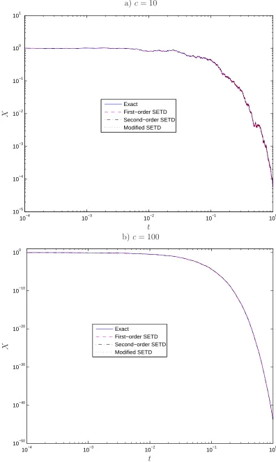
We conduct the simulation using α = 1, X0 = 1 and two large values of c, namely 10 and 100,

at ∆t = 0.0001. For all cases, a same set of random numbers over the time domain 0_≤ t _≤ 1 is

employed. Figure 3 shows profiles of the exact and computed solutions. It can be seen that the

the solution for the case ofc= 10 shows very small discrepancies between the approximate curves,

especially for 1st SETD and its modification. On the other hand, 1st SETD and its modification

are much more economic than 2nd SETD. At each time level, one needs to evaluate only three terms

for 1st SETD, two terms for its modification, but up to 5 terms for 2nd SETD. The corresponding

elapsed CPU times are 0.0019, 0.0017 and 0.0050 seconds, respectively (Intel CPU 2.40 GHz).

Furthermore, 2nd SETD requires an extra storage space to keep the value ofX at t₋∆t. Apart

from these, the time step used in the DPD method should be much smaller than the following time

scale [3]

tc =

rc

V =

√

mrc

√ 3kBT

≈O(√m), (48)

where V is the peculiar velocity. It implies that the maximum allowance time step decreases as

the particle’s mass is reduced, and the use of constant approximations over small time steps (i.e.

1st SETD and its modification) for low-mass DPD systems appears to be appropriate. For these

reasons, in simulating fluid flows by means of DPD, 1st SETD and its modification are preferred

options. Hereafter, they are denoted by SETD and MSETD, respectively.

3.2

Viscometric flows

We next consider Couette and Poiseuille flows, where analytic solutions are available. The flow

domain is chosen as Lx×Ly ×Lz = 40×10×30. We impose periodic boundary conditions in

the x and y directions and non-slip conditions at the two planes z = _±15. The latter is achieved

using frozen particles at the wall region and in addition, a thin boundary layer in which a random

velocity distribution with zero mean is enforced [4]. Furthermore, the particles are required to

leave the wall according to the reflection law proposed in [18]. The motion of a fluid is driven

by applying velocity vectors (_±7.5,0,0)T _{to particles in the two thin boundary layers at z =±15}

for Couette flow and by applying an external force vector (0.1,0,0)T _{to each particle inside the}

simulation domain for Poiseuille flow.

We conduct the simulation for two small values of mass, namely 0.1 and 0.01. Other DPD

param-eters used arerc = 1, aij = 18.5,σ = 3, kBT = 1, n= 4 and s= 1/2.

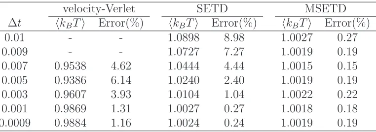
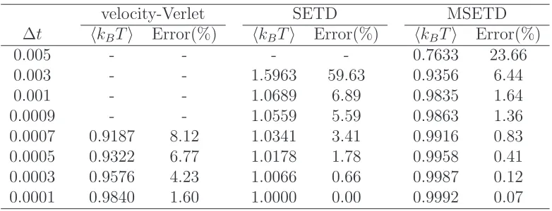
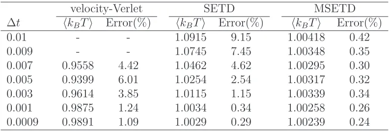
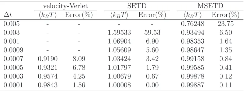
in Tables 3 and 4 for Poiseuille flow. For both flows, the present SETD and MSETD schemes

outperform the velocity-Verlet algorithm. Much larger values of time step can be employed with

SETD and MSETD than with the standart velocity-Verlet algorithm. The velocity-Verlet

algo-rithm fails to give a convergent solution at ∆t '0.009 and ∆t'0.0009 form = 0.1 andm= 0.01,

respectively. In terms of maintaining the equipartition principle, at a given small time step for

which the velocity-Verlet algorithm works, the ETD schemes yield the system temperature that is

in better agreement with the specified one, i.e.,kBT = 1, than the velocity-Verlet algorithm. For

m= 0.1 and with all time-steps considered, MSETD provides a solution whose error is quite small

(less than 0.3% for Couette flow and 0.5% for Poiseuille flow), always smaller than those produced

by SETD, and slightly fluctuating with time step (Tables 1 and 3). This fluctuating behavior is

probably due to the fact that the use of double-precision floating-point format may prevent the

method from achieving lower errors. For all cases, it can be seen that there is an improvement of

MSETD over SETD in the satisfaction of equipartition at a given time step. This enhancement

in the time-step size is attributed to the fact that the autocorrelation of the fluctuating part of

MSETD is slightly reduced at large time steps.

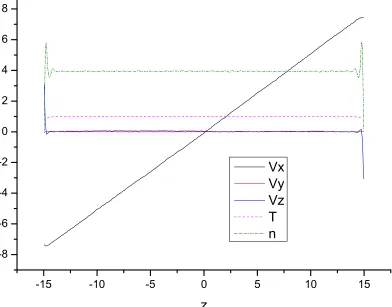
Results concerning the velocity field are presented in Figures 5 and 6 for Couette and Poiseuille

flows, respectively. It can be seen that profiles of linear and parabolic velocity are obtained. These

figures also show uniform distributions of the number density and temperature.

4

Concluding remarks

This paper reports some new integration schemes, which are based on the method of

exponential-time differencing and the Ornstein-Uhlenbeck process, for solving the DPD at low mass overdamped

limit. Salient features of the present schemes include (i) they do not contain unwanted fast time

scale associated with the stiff part and (ii) the autocorrelation of the fluctuating part has a very slow

variation at the high-end time-step region (i.e., c∆t _→1). These special features are particularly

suitable for the handling of overdamped systems.

We would like to thank the Referee for providing helpful comments and suggestions. This work is

supported by The Agency for Science, Technology and Research (A*STAR) through grant #102

164 0145. N. Mai-Duy also would like to thank the Australian Research Council for an ARC Future

Fellowship.

References

1. S. Chen, N. Phan-Thien, B.C. Khoo, X. Fan, Phys. Fluids 18(10) (2006) 103605.

2. P. Espa˜nol, Phys. Rev. E 52 (1995) 1734.

3. P. Espa˜nol, P. Warren, Europhysics Letters 30(4) (1995) 191.

4. X. Fan, N. Phan-Thien, S. Chen, X. Wu, T.Y. Ng, Phys. Fluids 18(6) (2006) 063102.

5. R.D. Groot, P.B. Warren, J. Chem. Phys. 107 (1997) 4423.

6. P.J. Hoogerbrugge, J.M.V.A. Koelman, Europhysics Letters 19(3) (1992) 155.

7. Y. Kong, C.W. Manke, W.G. Madden, A.G. Schlijper, J. Chem. Phys. 107 (1997) 592.

8. C.A. Marsh, G. Backx, M.H. Ernst, Phys. Rev. E 56(2) (1997) 1676.

9. W. Pan, B. Caswell, G.E. Karniadakis, Langmuir 26(1) (2010) 133.

10. I. Vattulainen, M. Karttunen, G. Besold, J.M. Polson, J. Chem. Phys. 116 (2002) 3967.

11. T. Shardlow, SIAM J. Sci. Comp. 24 (2003) 1267.

12. C. Marsh, Theoretical aspects of dissipative particle dynamics, D.Phil thesis, University of

Oxford, 1998.

13. D. Pan, N. Phan-Thien, N. Mai-Duy and B.C. Khoo, J. Comput. Phys. 242 (2013) 196.

14. N. Mai-Duy, D. Pan, N. Phan-Thien, B.C. Khoo, J. of Rheology 57(2) (2013) 585.

15. N. Mai-Duy, N. Phan-Thien, B.C. Khoo, J. Comput. Phys. 245 (2013) 150.

16. S.M. Cox, P.C. Matthews, J. Comput. Phys. 176(2) (2002) 430.

17. G.E. Uhlenbeck, L.S. Ornstein, Physical Review 36 (1930) 823.

Table 1: Couette flow: Comparison of the mean equilibrium temperature of the SETD, MSETD and velocity-Verlet algorithms for the case of m = 0.1. The velocity-Verlet algorithm fails to converge at ∆t'0.009.

velocity-Verlet SETD MSETD ∆t _hkBTi Error(%) hkBTi Error(%) hkBTi Error(%)

Table 2: Couette flow: Comparison of the mean equilibrium temperature of the SETD, MSETD and velocity-Verlet algorithms for the case ofm= 0.01. The velocity-Verlet and SETD algorithms fail to converge at ∆t'0.0009 and ∆t '0.0005, respectively.

velocity-Verlet SETD MSETD ∆t _hkBTi Error(%) hkBTi Error(%) hkBTi Error(%)

0.005 - - - - 0.7633 23.66

Table 3: Poiseuille flow: Comparison of the mean equilibrium temperature of the SETD, MSETD and velocity-Verlet algorithms for the case of m = 0.1. The velocity-Verlet algorithm fails to converge at ∆t'0.009.

velocity-Verlet SETD MSETD ∆t _hkBTi Error(%) hkBTi Error(%) hkBTi Error(%)

Table 4: Poiseuille flow: Comparison of the mean equilibrium temperature of the SETD, MSETD and velocity-Verlet algorithms for the case ofm= 0.01. The velocity-Verlet and SETD algorithms fail to converge at ∆t'0.0009 and ∆t '0.0005, respectively.

velocity-Verlet SETD MSETD ∆t _hkBTi Error(%) hkBTi Error(%) hkBTi Error(%)

0.005 - - - - 0.76248 23.75

10−10 10−8 10−6 10−4 10−2 100 0.92

0.93 0.94 0.95 0.96 0.97 0.98 0.99 1 1.01 1.02

c∆t

κ

10−2 10−1 100 10−5

10−4 10−3 10−2

Brownian motion First−order SETD Modified SETD

c∆t

h

∆

W

∆

W

i

a)c= 10

10−4 10−3 10−2 10−1 100

10−5 10−4 10−3 10−2 10−1 100 101

Exact

First−order SETD Second−order SETD Modified SETD

t

X

b)c= 100

10−4 10−3 10−2 10−1 100

10−50 10−40 10−30 10−20 10−10 100

Exact

First−order SETD Second−order SETD Modified SETD

t

X

10−0.257 10−0.256

10−2.42

10−2.41

10−2.4

10−2.39

Exact

First−order SETD Second−order SETD Modified SETD

t

X

-15 -10 -5 0 5 10 15 -8

-6 -4 -2 0 2 4 6 8

z

Vx

Vy

Vz

T

n

-15 -10 -5 0 5 10 15 -5

0 5 10 15 20 25

z Vx

Vy

Vz

T

n