The Development of Low-Order Models for the Study of Fluid-Structure Interactions

(1)

The Development of Low-Order Models for the Study of

Fluid-Structure Interactions

Thesis by

Andrew A. Tchieu

In Partial Fulfillment of the Requirements

for the Degree of

Doctor of Philosophy

California Institute of Technology

Pasadena, California

2010

(2)

c 2010 Andrew A. Tchieu

(3)

Acknowledgments

First and foremost, I would like to thank my advisor, Professor Anthony Leonard. He is a beacon

of kindness, has always been very supportive through all my endeavors, and genuinely cares for my

overall wellbeing. I can say without any doubt that his guidance and encouragement helped me

through many difficult times during my life. For that I am immensely indebted to him. It has been

an honor to be his student and a part of him will forever be instilled in me.

I would also like to express gratitude to my thesis committee members, Professors Beverley

McKeon, Tim Colonius, and Dale Pullin. I have had the pleasure to take courses from each one of

them and all have had an important part in my academic development.

I also want to thank several Professors associated with Caltech. Professor John Dabiri has been

inspiring and has taken the time to play on the Aero basketball team together with me among

other things. Professors Hans Hornung and Joe Shepherd have always been very interactive with

the members of our lab, constantly checking in to see how we are doing. In particular, I have

had the privilege to play tennis with a great tennis player in Professor Hornung, who consistently

outdueled me. Undoubtedly, he would have been a great tennis player if someone had not convinced

him to study fluid mechanics. Thanks to Professor Darren Crowdy who gave me several ideas that

contributed to the fourth chapter of this thesis. His enthusiasm for teaching has been contagious

and I hope one day to replicate his passion in the classroom.

I am also grateful to have interacted with all members of the Iris and Puckett Laboratories. In

particular, I met Hans Jonas as a visiting student in our lab, and he has been a great friend over

the past few years.

(4)

school and life in this perspective. Jeff Hanna has been the person that I possibly spend the most

time with here at Caltech, whether it be eating a lot of good food, drinking beer, or doing outdoor

activities (mainly running or biking). Emily McDowell has been a very good friend and I cherish

the dinners we have had talking about various things, both important and inconsequential. Dominic

Rizzo has been a constant source of humor and entertainment. Thanks to all my other friends at

Caltech, especially John Meier and Chris Kovalchick who I have had the pleasure of interacting with

on and off campus, whether it be biking or just having a meal. I would also like to thank Francis

Castillo and Kent Chau, who are two of my best friends from high school, for their support and

friendship. You are all good friends and have shaped me to be who I am today, and I thank you

from the bottom of my heart for being in my life.

I would also like to thank my girlfriend and best friend of all, Nancy Diep. I am the luckiest

man in the world to have found my soul mate. She has been exceptionally supportive through all

my mood swings while researching and writing my thesis. I will do everything in my power to make

you the happiest woman in the world.

Last, but not least, I would like to thank my mom, dad, brother, and sister. They, above all,

have been the most supportive throughout my whole education. When the times were rough, they

were the ones constantly listening and comforting me while I was complaining and being dramatic.

(5)

Abstract

In this work, several low-order models are derived to describe and simulate fluid-structure interaction

problems with rigid bodies at a modest computational cost. The models are based on the inviscid

flow assumption such that potential theory can be used with, in some cases, point vortices in the

flow. Three general areas of application are considered. First, a thin airfoil undergoing small-scale

unsteady motions in the presence of a freestream flow is investigated. The low-order model that is

developed has only one ordinary differential equation for the fluid dynamic variables. This model is

used to briefly investigate vortex-induced flutter in the attached-flow regime and control of a

free-flying airfoil using synthetic jet actuators. Second, the vortex-induced vibrations of an arbitrary

bluff body in the presence of vortices, with or without a freestream flow, are considered. Several

examples of the canonical mass-spring-damper system for a circular cylinder and a flat plate are

given to demonstrate the use of the vortex-based model for these applications. Finally, the

two-body problem in a potential flow is addressed. A relatively simple solution specific to the doubly

connected domain is determined and its resulting force and moment are coupled to the rigid bodies

to investigate the mutual interactions between the two bodies. Aspects of drafting behind a forced

body, the role of the fluid in elastic collision, and flapping flight are discussed in this context.

Although a few specific examples and applications are given for each chapter, the main purpose of

(6)

List of Figures

2.1 Schematic of the unsteady vortex dynamics model . . . 11

2.2 Schematic of the quasi one-dimensional simplification . . . 12

2.3 Summary of the low-order model . . . 24

2.4 Schematics of the NACA 4415 airfoil model and its free-flight test bed . . . 25

2.5 Comparison with experimental results for pure pitching . . . 27

2.6 Comparison with numerical simulations in pure pitch . . . 28

2.7 Vorticity field from DDES simulation demonstrating small-scale vortices shed off the non-sharp trailing edge (Lopez, 2009). . . 29

2.8 Comparison with numerical simulations in pure plunge . . . 30

2.9 Schematic for the vortex-induced flutter of a flat plate airfoil . . . 31

2.10 Various simulations of vortex-induced fluttering . . . 33

2.11 Case (e), a multi-modal response of a fluttering airfoil . . . 34

2.12 FFT of the response in Figure 2.11 plotted versus non-dimensional frequency . . . 35

2.13 Normalized vorticity plots of synthetic jets over a modified airfoil . . . 37

2.14 Numerical and theoretical evidence for shift in Kutta condition . . . 38

2.15 Change in lift versus change in moment due to control . . . 40

2.16 Relationship between ΓC,uC, andα . . . 41

2.17 Comparison of test bed simulation with experimental results . . . 42

2.18 Simple feedback is used to reduce induced vibrations . . . 44

(11)

3.2 Schematic of the application of Cauchy’s theorem to deform∂D0 . . . 55

3.3 Schematic of the vortex-induced vibration for a circular cylinder in cross flow . . . 58

3.4 Response of the system forz1(t= 0)/D= 0.930 with kz= 1 andbz= 0 att= 500 . . 61

3.5 Maximum amplitude versus vortex separation distance,z1/D . . . 62

3.6 Response of the system forz1(t= 0)/D= 1.275 andz2(t= 0)/D= 1.275iwithkz= 1 andbz= 0 att= 100 . . . 63

3.7 Schematic defining the parameters in the vortex street . . . 63

3.8 Max displacement versus Strouhal frequency of incoming vortex street . . . 64

3.9 Displacement versus time for St = 0.25 . . . 64

3.10 Schematic of the vortex-induced vibration for a flat plate in cross flow . . . 65

3.11 Schematic showing the instantaneous stagnation streamline at various instants of time 69 3.12 Streamlines at various instants in time for separated flow off of a plate at angle of attack 72 3.13 Evolution ofθ in vortex-induced vibration of a plate. . . 73

4.1 Two arbitrarily shaped objects in thez-plane mapped to the annulus in theζ-plane . 79 4.2 Instantaneous streamlines due to a cylinder approaching a fixed cylinder from the right at constant velocity. . . 88

[image:11.612.105.539.60.725.2]

4.3 Force coefficientCxwhen a cylinder moves toward a stationary cylinder as depicted in Figure 4.2 . . . 89

4.4 Instantaneous streamlines due to two cylinders approaching each other inline at con-stant velocity. . . 89

4.5 Magnitude of the force coefficient|Cx|when two cylinders move toward each other at constant velocity as depicted in Figure 4.4 . . . 90

4.6 Convergence of_|aj|2 versusj . . . 91

4.7 Several example paths of an aft cylinder following the forced motion of a forward cylinder 92 4.8 Contour plots for the force on an aft cylinder drafting behind another cylinder of equal radius . . . 93

(12)

with the second cylinder initially at rest . . . 98

4.12 Cylinder paths for a near-collision event . . . 99

4.13 Geometric quantities defining the configuration of two parallel plates inz-plane. . . . 100

4.14 Instantaneous streamlines for the flapping motion of two parallel plates with motion prescribed by Equation (4.33) . . . 101

4.15 Individual and total force and moment coefficients versus non-dimensinal time t∗ ₌ t/(2π) of two plates undergoing motion prescribed by Equation (4.33) for one cycle . 102 A.1 Simulink model for the simulation of the experimental apparatus . . . 110

A.2 Block diagram model for the wing aerodynamics . . . 111

A.3 Block diagram model for the torque motor . . . 111

B.1 Robust servo LQR with feed-forward element and added control signal . . . 120

B.2 Control hedging diagram . . . 125

B.3 ΓCwith control voltage saturation limits . . . 127

B.4 Diagram illustrating how the spring system interfaces to the wind tunnel model . . . 129

B.5 Verification that the static model models response with torque motor accurately . . . 130

B.6 Comparison between the vortex model and static model when the static model assump-tion fails . . . 131

(13)

List of Tables

2.1 Legend and list of parameters for various cases presented in figures 2.10 and 2.11. . . 32

(14)

Chapter 1

Introduction

1.1

Motivation and background

Research of fluid-structure interaction (FSI) has been an increasing area of active research, especially

with the ever-growing computational power of computers. Historically, the study of fluid dynamics

and structural dynamics, except for isolated examples, have remained partitioned. Methods involving

the study of fluid dynamics have relied on approaches where the fluid is treated without regard to

the dynamics of the structure such that walls or boundaries are fixed or moving with a prescribed

motion. Likewise, the study of structural dynamics has been, for the most part, studied without

coupling to a fluid although all terrestrial structures are submersed in a fluid. Although, some

information can be inferred using partitioned approaches, such as acquiring steady forces that a fluid

applies on a structure and subsequently determining the structure’s response, a coupled approach

may be necessary to accurately describe, simulate, and analyze the FSI problem. When the fluid

and structure are coupled through their mutual boundary conditions, the problem at hand becomes

increasingly difficult and the resulting fluid and structural motion may not be obvious.

FSI is ubiquitous in nature and daily life. The fluid-structure coupling between many of these

situations becomes crucial for the understanding of the phenomena and few examples are given here.

The quintessential example of coupled FSI is the induced instability resulting in the collapse of the

Tacoma Narrows Bridge in 1940. In this instance, von K´arm´an determined that the structural

(15)

governor of Washington to halt reconstruction in favor of redesigning of the bridge (von K´arm´an

and Edson, 1967). It can be claimed that this event itself paved the path for the advent of new

fields of study that include bridge aerodynamics and vortex-induced vibrations, which continue to

be extremely active areas of research. Perhaps the oldest and most well studied FSI problem, the

fluttering of airfoils has been studied for nearly a century due to the emergence of powered flight. Its

stability boundaries have been determined based on assumptions of periodic response and potential

flow assumptions (Theodorsen, 1935) yet there are still many more avenues for research.

In addition, FSI is important for a variety biological and naturally occurring situations. The

fluttering of flags and falling cards/leaves have been a source of constant interest (Michelin et al.,

2008, Eloy et al., 2007). In internal biological flows, the FSI of bi-leaflet mechanical heart valves is

studied to show that aorta geometry has a drastic effect on the opening and closing of the leaflets

(Borazjani et al., 2010, Eldredge and Pisani, 2008). Fluid-structure interactions have also been

essential in the study of locomotion of various genus such as fish, insects, and birds to name a few

(e.g. Triantafyllou and Triantafyllou, 1995). Moreover, the interactions of several bodies in proximity

have been studied in an effort to understand coordinated motion and passive locomotion (Nair and

Kanso, 2007, Kanso and Newton, 2009).

Since fluid-structure interactions are pervasive in everyday life, it is essential to distinguish when

the coupling of fluid and solid motions is important for the solution of the problem. When the

fluid and structure problems can be separated, the problem is drastically simplified which leads to

computational savings. Consider a fluid-structure problem where a deformable structure is immersed

in a fluid. There are time scales associated with the internal dynamics of the structure (e.g. elastic

waves), the motion of the structure (e.g. period of a flutter oscillation), and motion of the fluid

(e.g. vortex turnover time or convective time). If the time scale associated with internal dynamics is

much smaller than both the time scales of the motions of the structure and the fluid, then the elastic

effects of the structure can be neglected and the body can be modeled as being a rigid structure.

Although the study of flexible structures is a major interest in general, this thesis is restricted to

(16)

such that the unsteady motion of the fluid can be neglected because its effect is nearly instantaneous.

In this case, quasi-steady approximations can be used to determine forces and moments on the body

or bodies in place of solving the entire unsteady motion of the fluid in detail. The goal of this thesis

is to look at situations where this approximation cannot be made and thus the coupled problem of

the fluid and structure must be explicitly treated and solved with an unsteady model.

In many instances described above an incompressible assumption can be made without loss of

generality. Additionally, we can assume that the fluid is Newtonian so that the equations of motion

for the FSI problem forK rigid bodies can be written as

∂u

∂t +u· ∇u=−∇p+

1

Re∇

2_u _(1.1a)

∇ ·u= 0 (1.1b)

d2_x k

dt2 =Fk+Fe,k (1.1c)

d2_θ k

dt2 =Tk+Te,k (1.1d)

for each body k = 1,2, . . . , K where u is the velocity, pis the pressure, and Re is the Reynolds

number for the fluid. Each rigid body motion is completely chracterized by the location xk and

orientationθk. Fk,Tk,Fe,k, andTe,k are the force and torque due to the fluid (pressure and shear)

and external forcing, respectively. _Fk and Tk are not only functions of the fluid variables but are

also implicitly functions of the solid variables themselves. The boundary conditions for rigid body

motion are

u(x) =dxk

dt +

dθk

dt ×(x−xk), forx∈∂Dk. (1.2)

The most accurate method of predicting FSI of rigid bodies is to numerically solve equations

(17)

equations, two specific computational methods have been rather successful in the context of FSI. The

first uses body fitted grids to determine the fluid motion. In the case of rigid body motion, the flow

can be solved in a moving/rotating frame of reference for a single body (Wang, 2000). This cannot

be said with the introduction of several bodies. The second method to solve for the flow is to use

immersed boundary methods. Here a Lagrangian grid of the body is overlaid on top of the Eulerian

grid that is used for the solution for the fluid motion. The boundary conditions are interpolated

from the flow to the Lagrangian points and consequently a boundary forcing is required on the body

and is essentially diffused to the fluid in order to enforce the boundary conditions. Although initially

pioneered by Peskin (1972) there now exist various manifestations of this method (see Mittal and

Iaccarino, 2005, Taira and Colonius, 2007, for a review of various methods). To simulate FSI for rigid

bodies, both methods use a separate solver for the rigid body dynamics to partition the problem

into two distinct parts for each time step. Due to this fact, an iterative method is used to ensure

that the accelerations of the fluid and body are consistent, thus making the solution to the FSI

problem prohibitively expensive. When the mass ratio of the body compared to the same mass of

the displaced fluid is high, the numerical solutions of the fluid and rigid body dynamics can nearly

decouple from each other such that the iterative solver is unnecessary and an explicit solver can be

used in its place at a more modest computational expense. One must be careful about the strict

stability requirements on the time step in this case (Alben, 2008). When mass-ratios are low (or even

vanishing) however, special considerations are required to accelerate the iterative solver (Borazjani

et al., 2008). These low mass-ratio cases are extremely important for the study of vortex-induced

vibration of marine structures.

There are also several simplifications that can be made to reduce the computational expense that

seems to limit the effectiveness of simulating FSI at higher Re. For high Re, the viscous effects can be

neglected and thus equations (1.1) reduce to the incompressible Euler equations. This is equivalent

to interpreting that the increasing Re essentially confines the boundary layer to an infinitesimally

thin layer on the surfaces of the rigid bodies. Additionally, for structures with a long spanwise

(18)

in complex variables as determining an analytic complex potential,W = Φ +iΨ, such thatu=_∇Φ,

whereusatisfies the zero normal-velocity boundary conditions. Φ and Ψ are known as the velocity

potential and streamfunction, respectively. This greatly simplifies the problem to using the linear

superposition principle to add together individual elements of the flow. In the absence of vortex-like

structures, the solution can be determined without the need of solving any ordinary differential

equations. The most simple of these models is to use the potential to determine added-masses for

the treatment of a single accelerating body (Lamb, 1945, Newman, 1977). The treatment of the

FSI problem for this case in essence reduces to solving the rigid body dynamics equations with an

“added” mass that modifies the accelerations of the body. In the single rigid body case, the

added-mass is not time dependent. For several bodies, the coefficients are dependent on the instantaneous

configuration with respect to each other and thus are a function of time and are considerably more

difficult to treat (Kanso et al., 2005). A special case of the multiple body problem is studied in

Chapter 4.

Additionally, quasi-steady models have been proposed in place of determining the unsteady flow

around the bodies. The most prominent example of this is the use of the Kutta-Joukowski theorem

to predict that the unsteady forces, _F, on a single body will be ρfUΓ0 where ρf is defined as the

density of the fluid, U is the velocity associated with the body, and Γ0 is the circulation around

the body. The circulation itself must be determined either by applying a Kutta condition or using

some empirical information. For example Lighthill (1973) predicts the lift due to the Weis-Fogh

mechanism in insect flight using quasi-steady values of Γ0.

However, one of the shortcomings of this method is that it does not capture the required

un-steadiness in myriad situations where vortex-body interactions and vortex shedding are important

phenomena. Ideal point vortices (i.e. point singularities of vorticity) provide an ample

(19)

representation. They can be easily added to the potential and in general require a solution of an

or-dinary differential equation to determine its motion. Even with the added complexity of introducing

point vortices, the equations that represent the fluid in (1.1) are reduced to the solution of a finite

number of ordinary differential equations as opposed to solving a partial differential equation as in

the higher order methods presented above. Several studies have considered the body-vortex

interac-tion in the context of dynamical systems and the transiinterac-tion to chaos (Borisov et al., 2005, Roenby

and Aref, 2010). Shashikanth (2005) even reduced the general N-vortex, single-body problem to

become Hamiltonian in structure under special circumstances.

In cases involving viscous separation a sufficient model must be developed to capture its salient

features. For bodies with sharp edges, a quite natural model is to have the fictitious boundary

layer separate from the edge and form a sheet-like structure of concentrated vorticity. The vortex

sheet representation is first used by Clements (1973) to model flow separating from a square-based

section. The method is more rigorously pursued recently by Jones (2003) and Shukla and Eldredge

(2007) for fixed and flexible plates with prescribed motion. Unfortunately, the solution for the sheet

strength usually involves a non-trivial solution to an integro-differential equation which for FSI must

then be coupled to the equations of motion for the bodies (e.g. using the Birkhoff-Rott equations,

see Saffman, 1992, Pullin, 1978). A more simple model that is conducive to limiting the number of

fluid variables was previously proposed by Edwards (1954) and Brown and Michael (1954), among

others, where the entire vortex sheet is fundamentally rolled into a single vortex. After several years,

this method is then diligently employed to study and control some aspects of flow separation off a

semi-infinite and finite plate (Cortelezzi and Leonard, 1993, Cortelezzi et al., 1994, Cortelezzi, 1995,

1996). Many of these techniques are also adopted and extended by Michelin and Smith (2009b) for

use in several aspects of FSI.

The reduction of the problem to the use of discrete point vortices reduces the problem to solving

several ordinary differential equations with algebraic constraints (e.g. Kutta condition, conservation

of circulation). Because of the simple mathematical representation of the problem using discrete

(20)

This thesis focuses on introducing several low-order methods for the FSI with rigid bodies that

can be further used in a more rigorous manner to analyze and understand the stability and non-linear

behavior of the system. For now, a few examples are given along with the methods to demonstrate

the use of these techniques. The goal is to develop low-order models that describe several aspects of

FSI but at very modest computational cost. For example, these methods are ideal for use in rapid

prediction, optimization, and model-based feedback control design.

1.2

Thesis outline

This thesis is divided into three main chapters, each covering a distinctly different FSI situation

with a specific low-order potential model to combat the problem. To this end, Chapters 2-4 can

stand individually with little reference to one another. Although the author has made a modest

attempt to keep the notation consistent between all chapters, there may be small discrepancies that

may occur between them.

In Chapter 2 we derive a low-order model for a thin airfoil undergoing small-scale unsteady

motions in the presence of a freestream flow. The method is additionally coupled to the rigid body

dynamics and used to characterize some aspects of vortex-induced flutter. In addition, the model is

extended to account for synthetic jet actuators to control the free flight of the airfoil.

Chapter 3 discusses the development of a model for the vortex-induced interactions of an arbitrary

solid body with vortices either generated or pre-existing in the flow. This is specifically applied to

interactions of bluff bodies in the presence of freestream. Two specific examples are given in the

context of canonical vortex-induced vibration.

In Chapter 4 a method to handle the doubly connected two-body problem in a potential flow is

derived. The method is then coupled with the motion of the bodies. This method is used to analyze

(21)

example of two flat plates flapping is presented to demonstrate some aspects of unsteady bi-wing

flight.

Finally, in Chapter 5 we offer some concluding remarks and reiterate the main contributions of

this thesis. Several future directions of research are discussed for each specific model presented in

(22)

Chapter 2

A simple discrete-vortex model for

the non-uniform motion and

control of a thin airfoil

2.1

Introduction

Two-dimensional unsteady airfoil theory for incompressible flows has had a history that spans nearly

a century. The primary motivation for this work stems from a long interest in the prediction of

unsteady forces and moments for the control of aircraft and aeroelastic phenomena, for example the

flutter of aircraft wings. Although two-dimensional potential theory is a major simplification over

actual aerodynamics of thin bodies, it nevertheless gives insight into the underlying aerodynamic

mechanism of unsteady aerodynamics. The simplifications in complexity lead to a tractable problem

that can usually be handled by standard mathematical approaches and limited computing resources.

Because of the simplicity in two-dimensional potential theory, pioneering work was conducted

by Wagner (1925) to predict the initial response of an airfoil impulsively started from rest. This

work was extended by Glauert (1929) for predicting the force and moment on an oscillating airfoil,

but was left unfinished until it was first published with a complete solution by Theodorsen (1935).

Part of the general solution to the oscillatory problem is given by an analytical expression that

relates the effect of wake circulation on an airfoil lift in the frequency domain by the aptly called,

Theodorsen function. Similarly, several European researchers developed theories (K¨ussner, 1936,

(23)

to the Theodorsen function through a Fourier transform. Jones (1938) soon developed an operational

treatment for general airfoil motions in the Laplace plane based on on Fourier-integral superposition

of linear results for simple harmonic motion. Concurrently, von K´arm´an and Sears (1938) also

developed a more consistent method based on the integral equations resulting from a continuous

vortex sheet and Sears (1941) applied the method to several applications. An effective and thorough

review of the theories of Wagner, Theodorsen, Jones, and von K´arm´an theories can be found in

Bisplinghoff et al. (1955).

More recently there has been renewed interest centered on using finite approximations of

Wag-ner and Theodorsen functions. In particular, Edwards et al. (1979) derived geWag-neralized Theodorsen

functions relating motions of the circulatory part of the airloads to the motion of the airfoil and

ap-plied it to subcritical and supercritical flutter conditions. Peters (2008) gives additional information

on several finite state models predicting forces and moments in the frequency domain although one

major drawback of these methods is that they cannot be integrated in a fully coupled simulation of

the FSI. In addition, the models are rather mathematically complicated and in most cases are only

manageable for prescribed or assumed oscillatory motions.

The goal of this chapter is to create a low-order model for arbitrary thin airfoil motion and show

its efficacy in applications to various fluid-structure phenomena. Furthermore, this study addresses

the introduction of synthetic jet actuators for which a new model can be implemented for the control

of an airfoil. Because of this, it is chosen to use discrete vortices to model the mean effect of the

actuators. First, a tractable and simple aerodynamic model is presented to predict the forces and

moment on a thin airfoil undergoing arbitrary motions in the absence of any actuation. This model

is reduced to the solution of a single non-linear ODE and is validated with both experimental results

and detached-eddy simulation numerical testing. Next, using this simple model, the onset of

vortex-induced flutter of plunging and pitching airfoils is examined. Specifically, several examples are

given including one showing a multi-modal transient response. Lastly, the control of an airfoil with

synthetic jet actuators is investigated more closely. An actuator model is created and compared to

(24)

x

−a −c

2

Γi

. . .

Γ2

c

2 z1 α

z2

zi

Figure 2.1: Schematic of the unsteady vortex dynamics model of an airfoil undergoing arbitrary

motion in the presence of a freestream velocity. We note that the vortex strenghts Γi will have

alternating sign although here they are depicted to clarify the convention that positive circulation results in a vortex that rotates in the counter-clockwise sense.

feedback scheme is then used to control the aforementioned vortex-induced vibrations highlighting

one of many potential uses for the low-order model.

2.2

Aerodynamic model formulation

Here a model that is capable of predicting the forces and moments on a two-dimensional airfoil in

motion is developed. The work in von K´arm´an and Sears (1938) lays the foundation of non-uniform

motion of a thin airfoil by using the basic concepts of vortex theory available to an aeronautical

engi-neer without much of the “unnecessary mathematical complications” that are commonly associated

with the theories derived in the works of Theodorsen (1935) and Wagner (1925) among others. The

theory presented here has been generalized to account forany airfoil motion as long as it remains

small amplitude, as explained in Section 2.2.1, but closely follows the theory outlined in von K´arm´an

and Sears (1938) to make it as concise and clear as possible.

Consider the incompressible flow around a thin airfoil of chord lengthcin a free-stream with an

upstream velocity U∞ that flows from left to right. The airfoil undergoes an arbitrary motion in

both plunge and pitch defined by the body variablesyb andα, respectively. The pivot point for the

(25)

Nascent Vortex M(a)

x Γ2 . . . Γi

−a . . .

−c

2

Γ1

Constant Strength Vortices Vortex Sheet,γ(x)

U

xi

x2 y

x1 α

˙ yb

c

2

Figure 2.2: Schematic of the quasi one-dimensional simplification of Figure 2.2 after the application of assumptions given in Section 2.2.1.

motion of the airfoil by allowing the shear layer to separate into the wake as discrete and singular

elements of vorticity with circulation strength Γj at locationzj= (xj, yj).

2.2.1

Assumptions

Several assumptions are made so that a simple, closed-form, low-order model can be created to

predict the forces and moment on a thin airfoil. The assumptions are listed and explained as

follows:

1. The flow is considered high Reynolds number flow so that the boundary layer is sufficiently

thin and the viscous effects can be neglected. Furthermore, it is reasonable to assume that

the fluid remains irrotational except at the discrete points zj. This allows us to use the

potential flow description for the fluid. However, this leads to a conundrum since it is well

known that forces and moments depend largely on the vortex-like structures that arise from

viscous separation. Another view of the problem is to model the viscous boundary layer as

an infinitesimally thin vortex layer, which is still a solution to the Euler equations, and allow

this layer to separate into the flow at one or several discrete points (the details of separation

are discussed in Section 2.2.4). This pseudo-viscous mechanism allows us to introduce inviscid

(26)

2. Motions of the thin airfoil are considered small-amplitude so that the leading-edge separation

does not occur. This means that the characteristic motions must be h/c1 and ˙h/U∞1

where h is a characteristic length of the maneuver (in pitch this translates to α 1 and

˙

αc/U∞1 where the over-dot represents taking the time derivative of the quantity of

inter-est). Even when this is not the case, evidence in Lewin and Haj-Hariri (2005) suggests that for

a range of high frequency parameters (say with reduced frequencyk >5, wherek= 2πcf /U_∞

and f is the frequency of oscillation) the leading edge separation, although present, becomes

reabsorbed into the boundary layer and subsequently separates off the trailing edge. The

lead-ing edge separation in these instances does not affect the lift and moment characteristics as

severely as the trailing edge separation. In addition, the small-amplitude assumption allows

another drastic reduction in complexity. For small-amplitude motions, the departure of any

wake vortex elements in the transverse direction are considered small and thus the effect of

its transverse motion can be justifiably neglected. Thus the wake vortex dynamics can be

sufficiently restricted to their advection in a single dimension and the bound vorticity can be

adequately restricted to lie on thex-axis.

3. It is assumed that the leading-order unsteadiness of the thin airfoil can be modeled by the

motion of a flat plate. To take into account the effects of thickness and camber, the lift and

moment are modified in a quasi-steady fashion, that is, steady characteristics versus angle

of attack (AOA) are superimposed on the unsteady results for non-ideal airfoil shapes. This

allows a general theory that is applicable to the entire class of thin airfoils with very minor

modification using tabulated data, for instance, from Abbott and Deonhoff (1959).

These assumptions allow us to solve the drastically simplified problem depicted in Figure 2.2

(27)

x-axis. The schematic given in Figure 2.2 is not entirely one-dimensional because the boundary condition is applied on the vertical velocity such that the bound circulation reads

1 2π

Z c

2 −c

2 γ(s)

x₋sds=vb(x) +vv(x), on

c 2 < x <

c

2 (2.1)

where the functionvb is the apparent vertical velocity due to the body motion and instantaneous

AOA and vv is the velocity induced by any shed vortices. Note that the integral equations for

the sheet strength are evaluated in the principal value sense. Furthermore, if there are N discrete

vortices in the wake at any time, the bound circulation can be decomposed into

γ(x) =

N

X

j

γj(x) +γ0,t(x) +γ0,r(x) (2.2)

so thatγi(x) satisfies the boundary condition for an individual vortex in the wake, γ0,t(x) satisfies

the boundary condition due to plunging motion and the free-stream, andγ0,r(x) satisfies the

bound-ary condition solely due to rotation around its mid-chord, x = 0. It is also understood that the

distributions are all functions of time since the problem is unsteady at heart. We have elected to

drop the time dependence from the expressions for the bound circulation strengths understanding

that they are indeed a function of time.

2.2.2

Bound vortex circulation

Consider a discrete wake vortex that has separated from the plate with circulation Γj located at

x=xj. The details of its creation will be addressed later in Section 2.2.4. From assumption 2 in

Section 2.2.1, the vortex remains forever on the x-axis and only convects in the x-direction. The

influence of this wake vortex on the airfoil will result in the creation of a distribution of circulation

around the airfoil,γj(x), to satisfy the boundary condition that no flow penetrates the plate, i.e.

1 2π

Z c

2 −c

2 γj(s)

x₋sds= Γj

2π(x₋xj)

, on c 2 < x <

c

(28)

application of the Kutta condition forces

γj

x= c

2

= 0 (2.4)

and uniquely determinesγj(x).

The formula for the bound circulation density on the surface of the airfoil that satisfies both the

boundary condition (2.3) and the Kutta condition (2.4) is found in von K´arm´an and Sears (1938)

and is given as

γj(x) =

Γj

π(xj−x)

sc

2−x c 2+x

xj+2c

xj−₂c

. (2.5)

Equation (2.5) is derived by using conformal mapping and using the fact that the vortex lies on the

x-axis. The amount of circulation bound to the airfoil due to this distribution is

Z c

2 −c

2

γj(x) dx= Γj

s xj−₂c

xj+₂c −

1 !

. (2.6)

Note that the circulation of both the vortex and its bound circulation gives a net circulation due to

the enforcement of the Kutta condition. In comparison to other proposed methods, such as those

given in Graham (1983), Cortelezzi (1996), and Michelin and Smith (2009b), the bound circulation

presented here changes with position of the wake vortex. In these specific cases, the Milne-Thomson

(1968) circle theorem is used to model the separation and this produces an exact opposite bound

vortex on the body. When using the circle theorem, the strength of the nascent vortex is most easily

determined by the explicit application of the Kutta condition since the conservation of circulation is

automatically satisfied. Here we have chosen to model the separation such that each element satisfies

(29)

strength of the nascent vortex. This is just another example of the non-uniqueness in the treatment

of potential flow problems. With the application of both the Kutta condition and conservation of

circulation (discussed in Section 2.2.4) all approaches should yield identical results under the same

assumptions.

2.2.3

Quasi-steady bound circulation

Airfoil translation and rotation lead to an additional term that is deemed the quasi-steady bound

circulation about the airfoil. These circulation distributions due to airfoil motion are denotedγ0,t(x)

andγ0,r(x) for “translation” and rotation, respectively, and represent associated circulation densities

in the absence of wake vortices. For the “translational” term, a non-zero vertical velocity of the

airfoil measured from the mid-chord, ˙y−aα˙−U∞sinα, must be matched by an equal fluid velocity

to satisfy the no through-flow condition. Here the term “translational” is used loosely because the

terms that have no x-dependence have been lumped together. In this specific boundary condition

the free-stream component and additional rotational component are added, so that γ0,r(x) results

from a pure rotational motion at the half chord, x= 0. Assuming the small angle approximation

sinα_≈α, we requireγ0,t(x) to satisfy

1 2π

Z c

2 −c

2 γ0,t(s)

x₋sds= ˙y−aα˙−U∞α, on− c 2 < x <

c

2 (2.7)

where the integral is taken using principal-value integration. We find thatγ0,t(x), satisfying (2.7)

and the Kutta condition, is

γ0,t(x) = 2 ( ˙y−aα˙−U∞α) s_c

2−x c 2+x

(2.8)

from which we obtain the circulation moments

Γ0,t= Z c

2 −c

2

(30)

Similarly, airfoil rotation about the mid-chord produces an airfoil velocity−αx˙ to be matched by a

velocity induced by the circulation distributionγ0,r(x). Thus it is required that

1 2π

Z c

2 −c

2 γ0,r(s)

x₋sds=−αx,˙ on− c 2 < x <

c

2. (2.10)

The solution satisfying (2.10) and the Kutta condition is

γ0,r(x) =−2 ˙α r

c2

4 −x

2 _(2.11)

from which we obtain the moments

Γ0,r= Z c

2 −c

2

γ0,r(x) dx=−

πc2_α_˙

4 (2.12a)

Z c

2 −c

2

xγ0,r(x) dx= 0 (2.12b)

Z c

2 −c

2

x2γ0,r(x) dx=

c2

16Γ0,r. (2.12c)

The total bound quasi-steady circulation can be found by adding (2.9a) and (2.12a) to obtain

Γ0= Γ0,t+ Γ0,r=πc

˙ yb−

a+c

4

˙

α−U∞α

. (2.13)

2.2.4

Wake vortex dynamics

A few physical laws govern the wake vortex dynamics. First, the system must obey the conservation

(31)

zero circulation) therefore we have

Γ0+

N

X

j=1

Γj

s xj+₂c

xj−₂c

= 0. (2.14)

We recall that the total circulation due to a separated vortex and its associated bound circulation

is not zero and therefore contributes the second term in 2.14.

Next, in point-vortex dynamics, the convection velocity of each vortex depends on the mutual

influence of other vortices in addition to the influence of the body. Since the amplitudes of the

motions are assumed to be small and at a low reduced frequency, the convection of a free vortex

can be assumed to not be modified by the presence of other vortices. To first order this assumption

leads us to model the motion of all but the most recent of the free vortices to move with speedU∞,

i.e.

dxj

dt =U∞, forj≥2. (2.15)

The vortex nearest to the body (always indexedj= 1) is being fed circulation and moves with speed

dx1

dt =U∞−

x2 1−c

2

4

x1Γ1 !

dΓ1

dt (2.16)

where we have used a conservation of impulse argument to correct its motion due to the change

in its circulation. This is much like the corrections that have been used in Brown and Michael

(1954), Cheng (1954), Rott (1956), and more recently Cortelezzi (1992) and Michelin (2009), but in

this one-dimensional analogue the correction gives an initial lift characteristic that agrees well with

Wagner’s impulsive start solution.

Naturally, since the flow is at high Reynolds number, the strength of the vortices can be assumed

(32)

i.e. Γjremains constant once it is released from the trailing edge. The strength of the nascent vortex

is determined by the conservation of circulation. Therefore, from (2.14)

Γ1=−

s x1−c₂

x1+c₂  Γ0+

N

X

j=2

Γj

s xj+c₂

xj−c₂



. (2.18)

This now begs the question: when does a vortex become a free vortex? Since a vortex cannot

“unwind,” the magnitude of its circulation strength cannot ever decrease. This means that a vortex

only gets stronger or equivalently that ˙Γ1 does not change sign while the vortex is being fed

circu-lation from the trailing edge. Say the rate ˙Γ1changes sign att=te, then we model the physics by

introducing a new vortex such that the discrete vortices get re-indexed as Γj+1(t+e) = Γ1(t−e) and

xj+1(t+e) =x1(t−e) after which the nascent vortex gets reinitialized as Γ1(t+e) = 0 and x1(t+e) = c2.

2.2.5

Aerodynamic lift and moment

We derive the lift and moment from using the conservation of linear and angular impulse. The total

fluid impulse in they-direction,Iy, is given by

Iy =−ρf  Z c 2 −c 2

xγ(x) dx+

N

X

j=1

Γjxj



 (2.19)

where γ(x) =γj(x) +γ0,t(x) +γ0,r(x) is the total distribution of circulation about the airfoil and

ρf is the fluid density. Using (2.5), (2.19) becomes

Iy=−ρf  Z c 2 −c 2

xγ0(x) dx+

N X j=1 Γj r x2 j− c2 4 

(33)

The lift on the airfoil is defined as

L=₋dIy dt

=ρf

d dt Z c 2 −c 2

xγ0(x) dx−ρfU∞Γ0−

ρfU∞c 2 N X j=1 Γj q x2

j−c

2

4

(2.21)

where we have used Equations (2.14)-(2.16) to remove time derivatives on Γj andxj. The first term

on the right-hand side of (2.21) leads to the so-called added mass terms due to airfoil acceleration,

the second term is the quasi-steady lift, and the remaining sum represents the lift due to vortices in

the near wake. In the absence of body motion, the lift due to the wake is a weakly decaying function

that goes like _O(1/t) as time increases. Upon substitution of (2.9), (2.12), and (2.13), Equation

(2.21) becomes

L=ρfπ

−c

2

4y¨b−U∞cy˙b+ ac2

4 α¨+U∞c

a+c

4

˙

α+U_∞2cα

−ρfU₂∞c

N X j=1 Γj q x2

j−c

2

4

. (2.22)

Similarly, to derive an expression for the moment acting on the airfoil, the conservation of angular

impulse is employed. The total angular impulse,_A(s), at a distancesupstream of the mid-chord of

the airfoil is given by

A(s) =₋ρf

2  Z c 2 −c 2

(x+s)2γ(x) dx+

N

X

j=1

Γj(s+xj)2



. (2.23)

The counter-clockwise moment on the airfoil, M(a), about the pivot point distancea upstream of

the mid-chord is given by dA(s)/dt evaluated at s = a, where one must take into account that

ds/dt=₋U_∞. Thus we find that

M(a) = ρf

2 d dt  Z c 2 −c 2

x2γ(x) dx+

N

X

j=1

Γjx2j



+U_∞Iy+aL. (2.24)

(34)

Equa-+ρfU∞c 2 8 N X j=1 Γj q x2

j−c

2

4

−ρ₂f   

x2 1−c

2 4 3 2 x1 dΓ1 dt  

. (2.25)

It is recommended to neglect the last term of this expression above to agree with the classical

result that the lift force due to wake vorticity acts at the quarter-chord point of the airfoil with

no additional moment. Recall that the conservation of impulse is used to derive the velocity of the

nascent vortex. There are simply not enough variables to satisfy the conservation ofy component

of linear impulse, conservation of angular impulse, and the Kutta condition with the adjustment

of a single vortex (three governing equations and two variables, Γ1, x1). Since we do not conserve

the angular impulse we choose to ignore this last term to correct this oversight. Further applying

Equations (2.9) and (2.12) to (2.25) yields

M(a) =aL+ρfπ

_U

∞c2

4 y˙b+

c4

128α¨−

U_∞ac2

4 α˙−

U2

∞c2

4 α

+ρfU∞c

2 8 N X j=1 Γj q x2

j−c

2

4

. (2.26)

Upon non-dimensionalizing Equations (2.22) and (2.26) the lift coefficientCL= 2L/(ρfU_∞2c) is

CL=π

−_2Uc2

∞ ¨ yb− 2

U∞y˙b+ ac

2U2

∞ ¨

α+2a+c U∞ α˙ + 2α

−_U1

∞ N X j=1 Γj q x2

j−c

2

4

(2.27)

and the standard moment coefficient (with pitch up being positive)CM =−2M(a)/(ρfU_∞2c2) is

CM(a) =−a

cCL+π

−_2U1 ∞y˙b−

c2

64U2

∞ ¨ α+ a

2U∞α˙ +

1

2α

−_4U1

j−c

2

4

. (2.28)

Note well that when all time derivatives are negligible, we recover two classical results for steady

aerodynamic theory. From the Equation (2.27) the steady state lift reduces to CL,∞ = 2πα.

Fur-thermore, if the moment is measured about the quarter-chord, i.e. a = c

(35)

moment reduces toCM,∞ a= c4

= 0.

2.2.6

Integration in time

One may notice that the integration of (2.16) and (2.18) is not straightforward due to the inherent

singularity att=te, the time at which a new nascent vortex is formed. To circumvent this problem,

we outline a new strategy to determinexj and Γj with no approximations. From the conservation

of total circulation (2.14) we define a new variable

G(t)_≡Γ1 s

x1+₂c

x1−₂c

=₋Γ0−

N

X

j=2

Γj

s xj+c₂

xj−c₂

(2.29)

that can be considered known up to timet. In addition, (2.16) can be rearranged as

d

dt Γ1

r x2

1−

c2

4 !

= qx1Γ1U∞ x2

1−c

2

4

= x1GU∞

x1+₂c . (2.30)

Defining

H(t) = Γ1

r x2

1−

c2

4 (2.31)

Equation (2.30) can be written as

dH

dt =

2H+cG

2(H+cG)GU∞ (2.32)

where (2.29) and (2.31) are used to rewrite

x1=

2H+cG

(36)

Integrating (2.32) in place of (2.16) numerically is now straightforward. At every time step we check

to see whether ˙Γ1changes sign, and if a creation event occurs, the integration returns to the previous

timet=t−e and creates a new vortex as described in Section 2.2.4.

2.2.7

Quasi-steady camber and thickness corrections

For non-idealized airfoils, Equations (2.27) and (2.28) must be adjusted to take into account the

effects of a finite thickness and/or camber. These corrections can be modeled to be quasi-steady in

the sense that the main source of unsteadiness originates from the fluid dynamics for a flat plate-like

airfoil. For instance, in numerical experiments performed with a more sophisticated discrete vortex

model the wake structure is nearly independent of the shape of the airfoil as long as the separation

occurs at the trailing edge.

From experimental evidence, the steady state lift for a thin cambered airfoil is nearlyCL≈2πα

in the attached flow regime (for several examples see the database in Abbott and Deonhoff (1959),

pg. 449-670). As a result, the coefficient of lift is simply adjusted by itsα= 0 lift,CL,0 to read

CL0 =CL,0+CL.

As for the moment, since the aerodynamic center is near the quarter-chord for thin airfoils, it can

be assumed that the moment coefficient has no direct dependence on the AOA and therefore the

coefficient of moment can simply be adjusted by its quarter-chord value to read

CM,0 c

4 =CM,0+CM,

c

4

whereCM,c

4 =CM(a=

(37)

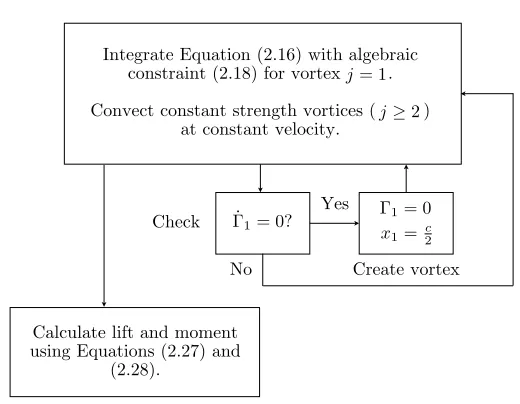
Integrate Equation (2.16) with algebraic constraint (2.18) for vortex .

Convect constant strength vortices ( ) at constant velocity.

Create vortex Yes

No

Check ˙Γ1= 0?

Γ1= 0

x1= c2

Calculate lift and moment using Equations (2.27) and

(2.28).

j_≥2

[image:37.612.193.453.66.268.2]

j= 1

Figure 2.3: A block diagram summarizing the low-order model.

In what follows, the prime notation is dropped with understanding that we are dealing with the

corrected values of lift and moment as presented above.

2.2.8

Summary of the low-order model

A block diagram summarizing the model is given in figure 2.3. To numerically simulate the model,

only one ordinary differential equation for the nascent vortex velocity, (2.16), must be integrated

with the constraint given by the conservation of circulation, (2.18). Equation (2.16) is replaced by

(2.32) to circumvent the singularity resulting from the introduction of a new vortex at the trailing

edge of the flat plate airfoil. All free vortices convect with constant strength and at the freestream

velocity therefore the locations of these vortices are determined analytically. At every time step, one

must check whether a new vortex is created based on the shedding criteria ˙Γ1 = 0. If ˙Γ1 changes

sign, then a new vortex is formed, the simulation is reinitialized to account for the formation of

a new vortex, and the simulation resumes. At any instant in time, the force and moment can be

determined from Equations (2.27) and (2.28). If necessary, the lift and moment are modified to

(38)

[image:38.612.127.533.85.291.2]

(a) (b)

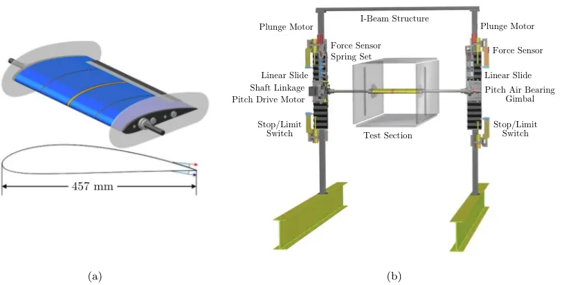
Figure 2.4: Depicted in (a) is the experimental model of the airfoil with modular synthetic jets attached and (b) is the experimental setup to allow for plunge and pitch control in an open-return wind tunnel facility at GTRI. Image is adapted from Muse et al. (2009).

2.3

Validation of the low-order model

The low-order model is compared to experimental results and numerical results of a NACA 4415

airfoil undergoing impulsive and sinusoidal pitch and plunge. This airfoil has been chosen primarily

due to its use at Georgia Technical Research Institute (GTRI) in Atlanta as the test bed for current

and future flow control experiments. The nominal values used here areCL,0= 0.4 andCM,0=−0.1.

2.3.1

Comparison with experiments

The experiments are conducted in an open-return low-speed wind tunnel having a square test section

measuring 1 m on each side using a modular airfoil fitted with endplates to limit its three-dimensional

effects. The airfoil model is depicted in Figure 2.4(a) and has a chord length of c= 0.457 m. The

wind tunnel model executes commanded flight maneuvers in two-degrees of freedom (pitch about

the quarter chord, a = 0.25c, and plunge) that can either be controlled by the combination of a

torque motor and linear vertical slides as schematically drawn in Figure 2.4(b) or by synthetic jet

actuators (as discussed in Section 2.5). Furthermore, the setup and control algorithms effectively

(39)

experimental setup and its control strategy can be found in Muse et al. (2008b) and Muse et al.

(2009).

For steady state measurements, the moment and lift are given by the torque motor and linear

slide load cells. When steady, measurements of the moment and lift are accurate with less than

1% error. An extension to the unsteady case is made for accurate estimation of the instantaneous

aerodynamic pitching moment and lift force during dynamic maneuvering. The moment is estimated

by using the dynamics equation

M =Iα¨− Te (2.35)

whereIis the measured moment of inertia and_Te =Kmumis the commanded motor torque withKm

andumbeing the motor torque gain and command input to the controller, respectively. The moment

of inertia is identified experimentally with less than 10% error. Angular acceleration ¨αis measured

with an angular accelerometer and its accuracy degrades with increasing pitching frequency and

therefore limiting the pitching frequency tofpitch<1 Hz. Estimation of the aerodynamic lift can be

done in a similar fashion but due to the several factors in the experimental design, the lift force is

much less accurately measured and, like the moment, its accuracy degrades with increasing plunge

frequency,fplunge. Because of this, the plunge mechanism is locked to remove the effects of inertia

and the lift force is measured directly from the load cell.

For the experimental test, the airfoil is pitched near quarter-chord at a free-stream Reynolds

number, Re = 9_×105_{, with a prescribed trajectory,}

α=αmaxsin

kpitchU∞ c t

(2.36)

where the amplitude, αmax, and reduced frequency, kpitch = 2πcf_U_∞pitch, are both functions of time.

As seen in Figure 2.5(a), a sinusoidal chirp signal is fed into the experiment such that the reduced

frequencies spanned range from 0.057 < kpitch < 0.068 (0.60 Hz < fpitch <0.71 Hz). The angular

speed of the airfoil is kept constant. Given in Figure 2.5(b) is the comparison of lift and moment

(40)

experimen-θ

˙_θ

¨θ

U t/c

0 500 1000

-10 0 10 -1 0 1 -0.5 0 0.5

α

˙

α

¨

α

Friday, July 2, 2010

(a)

CL

CM

U t/c

0 500 1000

-0.1 -0.05 -5 0 5

[image:40.612.175.432.126.578.2]

(b)

Figure 2.5: Comparison with experimental results for lift and moment for a NACA 4415 airfoil

pitching about its quarter chord. (a) Input data (in radians) from experiment (dotted, unfiltered ¨α).

Frequencies range from 0.057< kpitch <0.068 (0.60 Hz< fpitch <0.71 Hz). (b) Experimental and

model response: current model; experiments. Experimental results forCM were filtered

with a Butterworth filter to remove high frequency noise. Experimental results forCL are nearly

(41)

CL

CM

U t/c

2 4 6 8 10

[image:41.612.180.435.57.273.2]

-0.15 -0.1 -0.05 0 0.5 1

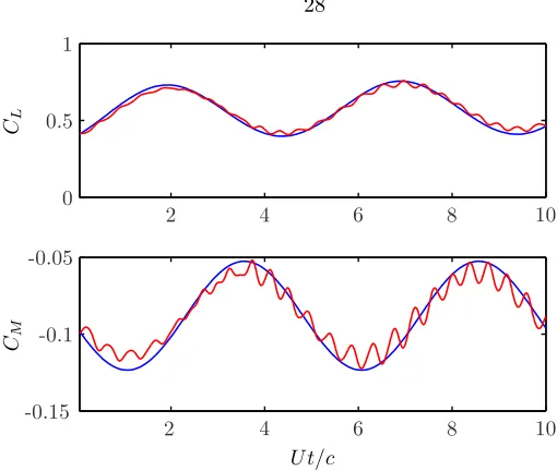
Figure 2.6: Comparison with high fidelity numerical simulations for lift and moment for a NACA

4415 airfoil purely pitching about its quarter chord with kpitch = 1.256 and 0◦ < α < 2◦: ,

current model; , DDES.

tal measured lift and the model lift is excellent. The experimentally measured moment (low-pass

filtered), shows slight departures from the model although the magnitude, frequency, and phase of

the dominant mode of oscillation is very well predicted. The differences between the two might

possible originate from the excessive noise in measuring the angular acceleration and using these

results in Equation (2.35). The agreement seen here is typical for frequenciesfpitch<1Hz.

2.3.2

Comparison with delayed detached-eddy numerical simulatons

Due to the limitations of the experimental facilities, numerical simulations are used to validate

models in situations not realizable by experimentation. In particular, higher pitch and plunge rates

are investigated. The numerical simulations presented here are computed at the University of Texas

at Austin using delayed detached-eddy simulations (DDES) by Lopez (2009). The DDES scheme

is a hybrid non-zonal Reynolds-averaged Navier-Stokes and large-eddy simulation scheme based

on the detached-eddy simulation model. For more information on the simulation, see Lopez (2009).

Simulations are run at a free-stream Reynolds number, Re = 9_×105_{, closely matching the conditions}

of the experiment.

(42)

Figure 4.7: Eddy viscosity (top) and vorticity field (bottom) atRe = 9_×105 _and

α= 0◦_{. (modified NACA4415)}

tions the slope is slightly negative. In this caseCdresults are in very good agreement

with experiments.

Figure 4.11 shows a comparison of the computational results between the

un-modified and un-modified NACA4415 profile. While theClcurve slope is not strongly

influenced by the geometrical modification of the airfoil profile, there is a radical

change to theCm curve slope. Changes in ∂C_∂αm have been observed experimentally

by De Salvo et al [37] with similar actuators but on a different airfoil section. An

important numerical parameter that can be computed from these results is∂Cm

∂Cl at low

angle of attack, which is related to the location of the aerodynamic center of the wing

81

Figure 2.7: Vorticity field from DDES simulation demonstrating small-scale vortices shed off the non-sharp trailing edge (Lopez, 2009).

pitching sinusoidally at a fixed frequency,kpitch= 1.256, which is more than two orders of magnitude

higher than the experimental case. The agreement here is acceptable given the simplifications made.

We notice that the simple low-order model cannot capture the small-scale oscillations that lie on

top of the gross lift and moment signatures. These high frequency oscillations can be explained by

vortex shedding off the non-sharp trailing edge in both the numerical simulations and the experiments

(although the sensors lack the resolution to resolve this) as seen in Figure 2.7. This causes small

amplitude von K´arm´an street to be shed from the trailing edge for all our operating conditions and

typically introduces a small asymmetry in the small-scale waveform due to its turbulent nature. Of

course, the low-order model cannot capture such an effect because of the prior assumptions made

in Section 2.2.1, but the model does capture the salient features, primarily reproducing the lift and

moment amplitudes, phase, and phase shift at the dominant frequency. The small-scale oscillations

in this case are considered negligible because under the standard operating conditions, the variations

in lift and moment due to the von K´arm´an street are _|∆CL| < 0.05 and |∆CM| < 0.01 and at a

frequency that is to high to garner a response when coupling with the fluid-structure interaction of

the rigid structure.

Figure 2.8 similarly shows the comparison for a fixed plunge angular frequency where the airfoil

heaves sinusoidally with an amplitude h= yb,max

c = 0.2. Again, the same trend is seen where we

have the small scale von K´arm´an shedding producing a small scale, high frequency signature in the

lift and moment. The results are still quite satisfactory in producing the essential characteristics in

(43)

CL

CM

U t/c

5 10 15

[image:43.612.175.443.57.281.2]

-0.2 -0.1 0 -1 0 1

Figure 2.8: Comparison with high fidelity numerical simulations for lift and moment for a NACA

4415 airfoil purely pitching about its quarter chord withkplunge = 1.256 and h= 0.2: , current

model; , DDES.

2.4

Vortex-induced flutter of a simple two degree of freedom

system

Consider a spring supported flat-plate wing section shown in Figure 2.9 with the a spring and damper

acting in the y-direction (ky, by) as well as in the angular direction (kα, bα). The model presented

above is applied to simulate the onset of vortex-induced flutter in the attached flow regime. The

dynamics of the system are modeled as

m∗by¨b∗+Sx∗α¨+by∗y˙b∗+k∗yy∗b=CL (2.37a)

Iα∗α¨+Sx∗y¨∗b+b∗αα˙ +k∗αα=CM(a) (2.37b)

where the equations of motion are non-dimensionalized following Leonard and Roshko (2001) with

yb∗=

yb

c , t

∗₌ tU∞ c , m

∗

b=

mb 1 2ρfc2

, Iα∗ =

Iα 1 2ρfc4

, S∗x=

Sx 1 2ρfc3

,

b∗y=

by 1 2ρfU∞c

, k∗y=

ky 1 2ρfU∞2

, b∗α=

bα 1 2ρfU∞c3

, k∗α=

kα 1 2ρfU∞2c2

(44)

k

α

b

α

U

Monday, September 13, 2010

Figure 2.9: Schematic of the vortex-induced flutter of a flat plate airfoil. The point at which the spring-damper is attached is also the pitching axis (refer to Figure 2.2).

The static imbalance, Sx, results from a body not pitching about its center of mass and for a

flat-plate wing section this can be reduced toSx =mbaassuming that the center of mass is near the

mid-chord (Naudascher and Rockwell, 1994). Additionally, for a flat plate, the mass moment of

iner-tia can also be analytically expressed asIα=mb

a2₊c2

12

. It is noted that non-dimensionalization

in this fashion is different from the traditional formulation (for example see Williamson and

Go-vardhan, 2004) but as explained in Klamo (2007) the non-dimensionalization with fluid dynamic

parameters are compatible with the traditional formulation. In what follows the (∗_{) is dropped with}

the understanding that all values are in their non-dimensional form.

Upon substitution of (2.21) and (2.26) into Equations (2.38) and (2.39), the motion of the airfoil

is dictated by two additional ordinary differential equations

mb+π

2

¨

yb+ (by+ 2π) ˙yb+kyyb+

Sx−aπ

2c ¨ α +

1 +2a

c

πα˙ + 2πα=−_U1

j−c

2

4

(2.38)

Sx−

aπ 2c

¨ yb+

_c −4a

2c

πy˙b+

Iα+π

₁ 64+ a2 2c2 ¨ α+ bα+

aπ(4a+ 3c)

2c2 ˙ α +

kα+

π(4a+c) 2c

α=₋ 1

4U∞ N X j=1 Γj q x2

j−c

2

4

. (2.39)

(45)

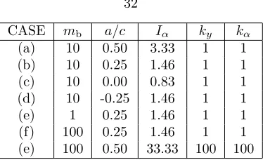
CASE mb a/c Iα ky kα

(a) 10 0.50 3.33 1 1

(b) 10 0.25 1.46 1 1

(c) 10 0.00 0.83 1 1

(d) 10 -0.25 1.46 1 1

(e) 1 0.25 1.46 1 1

(f) 100 0.25 1.46 1 1

[image:45.612.231.418.57.171.2]

(e) 100 0.50 33.33 100 100

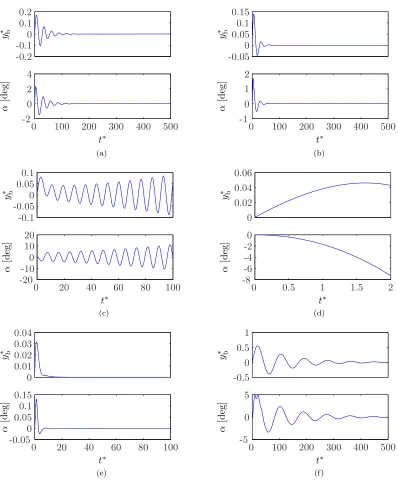
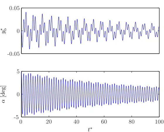
Table 2.1: Legend and list of parameters for various cases presented in figures 2.10 and 2.11.

response of the system.

Although many studies revolve around determining the general stability of the system (e.g. the

lowestU∞= ˜U∞ such that the airfoil remains flutter free), due to the large parameter space, it is

nearly impossible to come to any general conclusion. In particular, Bisplinghoff et al. (1955) could

only draw a few generalizations after conducting several parametric studies using a fully periodic

response assumption. In addition, the highly non-linear behavior of the wake vortices makes it

difficult to determine a closed form solution to the problem such that a definitive stability analysis

can be performed. Instead, the focus here is to look at a few key responses to highlight the transient

and multi-modal behavior of vortex-induced flutter.

We take a look at undamped structures such that both by and bα are set to zero. Typical

aircraft structures have mass ratios mb = O(10−100) and stiffnesses, kα = O(0.1 −100) and

ky=O(0.1−100).

Figure 2.10 gives several responses due to artificially induced gust in they-direction with a list

of parameters for these cases given in Table 2.1. The gust is modeled in the simulation by setting

the initial condition ˙yb= 0.05, i.e. 5% of the free-stream velocity.

In cases (a)-(d), the pitching axis is gradually moved from the leading edge towards the trailing

edge, thus also changing its mass moment of inertia,Iα. It is observed in 2.10(a) when held at the

leading edge, the vibrations in the structure are stable for this set of parameters. As one moves

back towards the quarter-chord, Figure 2.10(b), the oscillations are further suppressed. When the

pitching axis is moved to the mid-chord and further, Figure 2.1

The Development of Low-Order Models for the Study of Fluid-Structure Interactions