Measuring strain using microwave energy

(1)

University of Southern Queensland

Faculty of Health, Engineering and Sciences

Measuring Strain Using Microwave Energy

A thesis submitted by

M. Trethewey

in fulfilment of the requirements of

Master of Engineering Research

(2)

Abstract

The measurement of force (or weight) is required in a great diversity of industries

and applications. The wide range of force levels, force characteristics and required

data has driven the development of many different technologies to meet these needs.

Most of these technologies depend on the force (or weight) deforming an elastic load

bearing member, with some form of transducer to convert the strain in the member

to an electrical quantity. The selection of this transducer will depend heavily on the

particular application. The range of major technologies are briefly reviewed and their

limitations noted.

The research set out in this dissertation investigated an original transducer system that

uses microwave energy to measure the strain in a loaded member, with the member

forming an integral part of the transducer. The basic design principle involves a pair

of cavities in the elastic member, one only which is subject to deformation under load,

while both cavities share a common temperature profile. The cavities are caused to

resonate by a microwave feedback exciter, and the difference frequency between the

cavities is extracted. This difference frequency will carry information related to the

strain in the loaded cavity, whilst discriminating the common mode dimensional changes

due to expansion and contraction with temperature change.

The design of a prototype transducer system focused on three areas:

The mechanical design of a transducer which produced strain in the loaded cavity in one

co-ordinate direction only, so as not to produce complex deformation of the cavity. In

principle this would ensure good linearity between the applied load and the microwave

(3)

ii

experience no strain when the first cavity was loaded, but both cavities were adjacent

in a single block of metal to ensure a common temperature profile. This member

was designed to meet all the normal requirements, specifically low creep, high fatigue

life and good stress-strain linearity within Hooke‘s law, but also had to be suitable for

manufacture in a material having low resistivity to maintain high Q values in the cavity

resonators. The readily available Alloy-380 brass was chosen.

Electromagnetic analysis was undertaken for both shallow cylinder and shallow square

box cavities, and the methods of electrically coupling into each. The resonant frequency

sensitivity to cavity deformation in different co-ordinate directions and modes of

reso-nance was also analysed. The advantages and disadvantages of each, and the choice of

a suitable cavity resonant frequency is discussed.

Microwave system design comprised a loop feedback type microwave oscillator using

MMIC (monolithic microwave integrated circuit) devices as the active components.

The phase and magnitude data for coupling between the cavity probes is detailed,

and an analysis of the design procedure for the printed circuit board microstrip layout

is described. The difference frequency between the two cavities was extracted using

a microwave mixer, and its design is detailed including the local oscillator and the

intermediate frequency amplifier.

Two aspects of performance verification of the design were undertaken. Firstly,

res-onator performance measurements were undertaken and analysed with respect to the

performance of the microwave equipment available. Measurements revealed the

charac-teristics of the coupling probes in the cavity, the performance of signal output coupling

alternatives between the cavity and the effects of circuit shielding. The principal results

were:

• Phase noise = -50 dBc/Hz (relative to carrier) at 1 kHz offset from carrier

• 3 dB bandwidth = 2 kHz

• Drift = -0.0055% of carrier / 5 minutes

(4)

iii

Secondly, the performance of the complete prototype transducer was measured.

Appa-ratus to load the transducer was designed and constructed, and the output difference

frequency between the two cavities monitored during progressive loading and

unload-ing, and independent repetitions provided an assessment of repeatability. The results

yielded a sensitivity of 4.84± 0.05 and 4.79±0.05 kHz/kg wt (respectively), at least 99.9% linearity, and nil detectable hysteresis (i.e. less than the limits imposed by the

measuring equipment).

It is concluded that the technique is feasible and proof-of-concept has been achieved,

but there remain significant challenges before the technique would be commercially

(5)

Certification of Dissertation

I certify that the ideas, designs and experimental work, results, analyses and conclusions

set out in this dissertation are entirely my own effort, except where otherwise indicated

and acknowledged.

I further certify that the work is original and has not been previously submitted for

assessment in any other course or institution, except where specifically stated.

M. Trethewey

Q9521089

Signature of Candidate

Date

ENDORSEMENT

Signature of Supervisor/s

(6)

Acknowledgments

I wish to thank my three supervisors Assoc. Prof. Nigel Hancock, Dr. Andrew Maxwell

and Assoc. Prof. Jim Ball for their untiring support and responses to my questions.

Without their input this project would not have been possible. I would also like to

make particular mention of Assoc. Prof. Jim Balls’ knowledge of microwaves and his

willingness to participate in this project in his retirement.

Thanks to Prof. John Leis who provided a great deal of encouragement for me to

commence this project and help in organising the initial meetings with academic staff

and help with the research training training scheme scholarship.

I would also like to thank my beautiful wife Deanne for her support and understanding

throughout this project.

M. Trethewey

University of Southern Queensland

(7)

List of Figures

2.1 Conceptual layout of cavity with two orthogonal resonators - reproduced

from Fig 8.Farley et al. (1991) . . . 8

2.2 View of the Farley et al. (1991) cavity cross section under load - repro-duced from Fig 5. . . 9

2.3 Setup of the Barth (2000) feedback oscillator clearly showing the two coupling ports into the cavity - reproduced from Fig 1(a). . . 16

2.4 Oscillator Equivalent Circuit : partly reproduced from Materka & Mizushina (1982) . . . 19

2.5 Tapered Stripline Transformers reproduced from Womack (1962) . . . . 21

2.6 Variation of F(ω) with frequency for various values of the ratio _βδ o re-produced from Womack (1962) . . . 22

2.7 Two-port transistor oscillator circuit - reproduced from Kai Chang & Nair (2000) . . . 23

3.1 Simple Cantilever Beam . . . 28

3.2 Simple Beam with Two Cavities . . . 29

(14)

LIST OF FIGURES xiii

3.4 Displacement of Beam with Strain Control Holes. The colour bar shows

displacement in meters. . . 31

3.5 Displacement of Bending Type Beam under load . . . 33

3.6 Compression Block Design Drawings . . . 34

3.7 Compression Block Simulation Results . . . 35

3.8 Picture of Cavities . . . 37

3.9 Picture of the Cavity Probe and SMA Connector . . . 37

3.10 Picture of the Probe and Cavity Cover Plate Assembly . . . 38

3.11 Picture of the Complete Cavity Assembly . . . 38

3.12 Comparison between Impedance Phase and Magnitude for 40 mm Cavity with 3 mm Probe . . . 39

3.13 Comparison between Impedance Phase and Magnitude for 40 mm Cavity with 5 mm Probe . . . 40

4.1 Drawing of Dual Cavity Mechanical Block . . . 46

4.2 Constraints Applied to Dual Cavity Mechanical Block for Finite Element Analysis . . . 47

4.3 Strain Induced in Dual Cavity Mechanical Block due to Applied Loads . 48 4.4 S-N Diagrams reproduced from Oberg, Jones & Horton (1987). Diagram 1 shows the behavior of a material for which there is an endurance limit Sen. Diagram 2 shows the behavior of a material for which there is no endurance limit . . . 50

(15)

LIST OF FIGURES xiv

4.6 Stress-concentration factor, Kt, for a shaft, with a transverse hole, in

torsion - reproduced from Oberg et al. (1987) . . . 52

4.7 Modulus of Elasticity verses Temperature for Naval Brass : from Reed & Mikesell (1967) . . . 55

5.1 Electric Field Distribution for two modes of resonance - reproduced from 62 5.2 Electric Field Probe Coupling Impedance - second cavity port is termi-nated to 50Ω by S-parameter test unit . . . 64

6.1 Block Diagram of the Microwave Circuit . . . 70

6.2 Block Diagram of the Oscillator Circuit where Pc is the phase change between the cavity coupling probes and Pm is the phase change across microstrip traces on the printed circuit board. The MMIC amplifier will also have a phase change Pa between its input and output (not shown in figure) . . . 71

6.3 Plot of S21phase shift and magnitude between coupling probes in cavity running in TE(2,1,0) mode . . . 74

6.4 leq2 Diagram reproduced fromVisser (2007) . . . 76

6.5 lshortest Diagram reproduced from Visser (2007) . . . 77

6.6 Layout of Critical Phase Controlling Microstrip . . . 78

(16)

LIST OF FIGURES xv

6.8 Circuit Diagram of the Cavity Resonantor . . . 84

6.9 From left to right: R.F. Resonator, L.O. Amplifier in center with mixer

at the top, and L.O. Resonator . . . 85

7.1 Picture of Test Cavity and Cover Plate with SMA connector probes shown 90

7.2 Picture of Test Cavity with Cover Plate fitted and SMA connectors visible 91

7.3 Picture of Front and Back of SMA connector shorted to measure

electri-cal length of test setup . . . 92

7.4 S11 measurement of cavity probe 1 with cavity probe 2 tied to 50 ohms 93

7.5 S22 measurement of cavity probe 2 with cavity probe 1 tied to 50 ohms 94

7.6 Plot of Phase shift between cavity probe 1 and 2 verses frequency . . . . 95

7.7 Plot of coupling between cavity probe 1 and 2 verses frequency . . . 96

7.8 Circuit Diagram of the Transducer . . . 98

7.9 Connection of the Cavity Oscillator to the HP8565A Spectrum Analyser 100

7.10 A Pair of Spectrum Measurements of Cavity Resonator Output at 1 kHz

Resolution Bandwidth and 2 kHz frequency span per division . . . 108

7.11 Spectrum Measurement of Cavity Resonator Output at 1 kHz Bandwidth

and 10 kHz frequency span per division . . . 109

7.12 Spectrum Measurement of Cavity Resonator Output at 1 kHz Bandwidth

and 2 kHz frequency span per division with an approximate overlay of

the average signal . . . 110

7.13 Picture of Plastic Shielding Assembly . . . 111

(17)

LIST OF FIGURES xvi

7.15 Picture of Complete Printed Circuit Board Assembly . . . 113

7.16 Picture of Complete Transducer . . . 113

7.17 Picture of Redesigned Transducer with Brass Shield Fitted . . . 114

7.18 Picture of brass shield removed from transducer, showing conductive foam resonance absorbing material inside . . . 115

7.19 Close-up view of printed circuit board assembly to the transducer show-ing the mechanical isolatshow-ing gap . . . 116

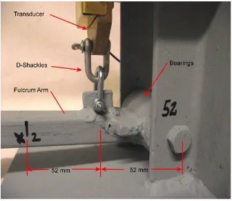
8.1 Picture of the test jig showing load weight, power supply and test equip-ment . . . 118

8.2 Close-up View of test jig showing locations of Transducer, D-shackles, Bearings and Fulcrum arm. Also shows major dimensions. . . 119

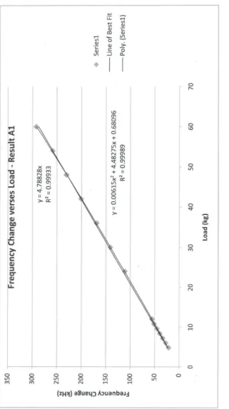
8.3 Graph of A1 results . . . 122

8.4 Chart comparing the means from data group A and B, also showing standard deviation error bars . . . 125

8.5 Graph of Hysteresis Measurement Results . . . 129

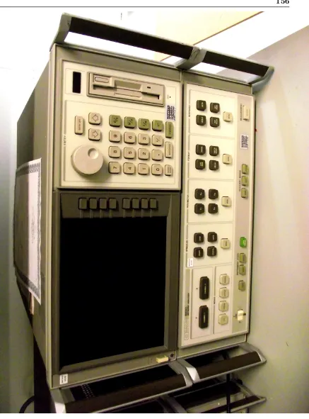
B.1 Picture of the complete group of microwave instruments . . . 155

B.2 Picture of the HP8510C Network Analyser . . . 156

B.3 Picture of HP8510C calibration tags . . . 157

B.4 Picture of the HP8514A S-parameter test set and the HP8350B sweep oscillator with HP83592A RF plug in . . . 158

B.5 Picture of HP8350B calibration certificate . . . 159

(18)

LIST OF FIGURES xvii

B.7 Picture of HP8510C calibration standards and connectors . . . 161

C.1 Result A1 Laboratory Table . . . 164

C.2 Result A1 Graph . . . 165

(19)

LIST OF FIGURES xviii

C.21 Result B1 Laboratory Table . . . 184

C.22 Result B1 Graph . . . 185

(20)

LIST OF FIGURES xix

C.41 Hysteresis Results Laboratory Table . . . 204

(21)

List of Tables

4.1 Ratio of Strength at Elevated Temperature Compared

to Strength at 21℃expressed as a Percentage . . . 49

7.1 Measured Signal Level for various Coupling Resistor Values . . . 99

7.2 Cavity Resonator Phase Noise Levels . . . 101

7.3 Drift of Cavity Resonator Frequency over Time . . . 102

7.4 Drift of Cavity Resonator Frequency over Time . . . 103

7.5 Drift of Transducer Intermediate Frequency over Time . . . 104

8.1 Data Collated from Group A Test Results . . . 123

(22)

Chapter 1

Introduction

1.1

Background

Modern society requires a very diverse range of weight and force measurements and

to meet this demand an equally diverse range of measurement technologies has been

developed. These technologies range from methods to determine the mass of

sub-atomic particles, right through to means of weighing bulk materials of many thousands

of tonnes. Some systems require extremely rapid response and settling times, while

others have more relaxed requirements. Yet other systems respond only to impulse

loads and discriminate static loads. In fact there are too many variations of system

requirements to mention here. The important point is that no single system can ever

cover all possible applications, so having available a diversity of technology options to

choose from for some particular weighing or force measurement application is vital.

The technology described in this dissertation relates to a technology that is intended to

offer another alternative, rather than being a replacement for any existing established

technology.

1.2

Hypothesis

(23)

1.3 Research Aims and Objectives 2

That the resonant frequency of a microwave cavity is set by its physical dimensions and

mode of resonance, and that changing the physical dimensions will change the resonant

frequency. So if the cavity is an integral part of a load bearing member, and strain is

induced in the member due to applied load, and the cavity is judiciously placed in the

member its physical dimensions will change. Thus by monitoring the cavity resonant

frequency, the strain in the load bearing member can be monitored, and transduction

from force (or load) applied to frequency has occurred.

Thermal changes in the load bearing member will cause changes in the physical

dimen-sions of the cavity due to expansion and contraction. It is proposed that this can be

discriminated from the desired signal by placing two cavities in the load bearing

mem-ber, one of which is strained by applied load and the other which is not. If the output

frequency is the mathematical difference between the two cavity resonant frequencies,

then the common mode temperature induced signal will cancel. The cavities must be

arranged to share a common thermal profile.

Using the difference frequency between the two cavity resonant frequencies should

pro-vide the added benefit of translating the microwave frequency signals in the cavities

down to much lower frequencies, without losing any of the desired information. This

would allow the use of lower cost electronics to process the output signal.

1.3

Research Aims and Objectives

There were five core aims and objectives in this research and they are detailed in the

sub-sections below.

1.3.1 Mechanical Member

The aim was to discover a mechanical design for a transducer which produces strain

in the loaded cavity in one co-ordinate direction only, so as not to produce complex

deformation of the cavity. In principle this would ensure good linearity between the

(24)

the second cavity needs to be arranged to experience no strain when the first cavity

was loaded, but both cavities must be adjacent in a single block of metal to ensure

a common temperature profile. This member needs to be designed to meet all the

normal requirements, specifically low creep, high fatigue life and good stress-strain

linearity within Hook‘s law, but also has to be suitable for manufacture in a material

having low resistivity to maintain high Q values in the cavity resonators.

1.3.2 Cavity Exciter Circuit

Due to the finite Q of any practical resonant circuit, an exciter must be used to maintain

resonance. There are a number of systems used in the past, but modern active and

passive components and surface mount manufacturing techniques make loop feedback

type exciters with electric field coupling probes a likely choice.

An electromagnetic analysis needs to be undertaken for both shallow cylinder and

shallow square box cavities, and the methods of electrically coupling into each. The

resonant frequency sensitivity to cavity deformation in different co-ordinate directions

and modes of resonance should also be analysed. The advantages and disadvantages of

each, and the choice of a suitable cavity resonant frequency will be reported.

As previously mentioned, a possible microwave system design comprises a loop

feed-back type microwave oscillator using MMIC (monolithic microwave integrated circuit)

devices as the active components. The phase and magnitude data for coupling between

the cavity probes must be detailed, and an analysis of the design procedure for the

printed circuit board microstrip layout described.

1.3.3 Performance of Cavity Resonator

The microwave cavity resonators are a vital component in the transducer, and good

performance of the resonators is critical. Any noise, jitter or poor spectral response of

the resonators will translate directly into the output signal, degrading the quality of

(25)

A test cavity needs to be constructed, along with coupling probes and exciter circuit.

This can then be used to measure key resonator performance indicators like:

• Centre Frequency

• Phase Noise

• 3 dB Bandwidth

• Drift

1.3.4 Construction of Complete Transducer

To achieve proof-of-concept a complete transducer unit needs to be constructed. This

would include the mechanical member with two cavities, exciter circuits and a

mi-crowave mixer, local oscillator and the intermediate frequency amplifier to extract

cav-ity resonator difference frequency signals. The microwave mixer, mixer local oscillator

amplifier, intermediate frequency amplifier and Faraday shielding must all be designed

and constructed.

1.3.5 Performance of Transducer

To test the transducer performance a jig needs to be designed and constructed to allow

known repeatable loading of the transducer. Sets of load tests should be performed

with the transducer output frequency monitored under each load condition. Analysis

of this data should provide the following:

• Frequency output change to load sensitivity

• Standard deviation of sensitivity

• Linearity

• Hysteresis

(26)

1.4 Structure of the Dissertation 5

1.4

Structure of the Dissertation

The dissertation comprises the following chapters:

• Introduction

• Literature Review : investigates previous work on using microwave cavity

res-onators to measure force, and loop feedback type exciters. Negative resistance

exciter systems are also reviewed.

• Initial Design Concepts and Microwave Cavity Measurements : details some initial

work on cantilever beam type mechanical members and a variety of other concepts

for the mechanical member.

• Mechanical Design of Transducer : reports on cavity geometry, properties of the

material in the member, and a mechanical design analysis of the chosen design.

• Microwave Resonator Theory : covers the choice of resonator frequency, resonator coupling, and resonator modes and sensitivity to cavity strain.

• Microwave System Design : describes the design procedure for the cavity exciters,

mixer local oscillator amplifier, microwave mixer and intermediate frequency

am-plifier.

• Resonator Performance : has a section that investigates the suitability of test

Equipment used, then details the tests and results of cavity resonator

perfor-mance.

• Prototype Transducer Performance Testing : introduces the test Equipment used,

method and results; and then provides a detailed analysis of the data.

(27)

Chapter 2

Literature Review

2.1

Introduction

The oldest archaeological evidence for weighing scales dates back to 2400 BC to 1800

BC, where polished stone cubes have been found in the Indus river valley (now Pakistan)

(Feuerstein et al. 2001). These cubes bear no markings, but their weights are multiples

of a common denominator. These stones were most likely used in a balance scale to

determine absolute weight, but it is thought that some form of balance scale was used

long before this to measure relative weight.

A simple cheap variant of the balance scale called a bismar became common around 400

BC, and was used by merchants (Crawford 1984). The bismar was a simple beam with

a fixed weight one end and a hook on the other end to attach the object to be weighed.

A handle with a knife edge pivot was used to suspend the unit, and the position of the

handle was adjusted until the beam was in balance. The weight of the object was then

read from calibration marks on the beam.

There are references to spring scales as early as 1600 AD, but the first reliable record

credits Richard Salter with the invention in 1770. By 1840 spring scales were in common

use due to the invention of the candlestick scale by R.W. Winfield (Graham 2003).

(28)

2.2 Measuring Mechanical Strain using a Cavity Resonator 7

atoms through to loads in ocean going bulk carriers. There is a great variety of

tech-niques and devices to perform these functions, and no single device fits all applications.

This document describes one technology variant for weighing, and is intended to

inves-tigate its potential as an additional option that may provide some unique advantage

for a specific application, rather than a replacement for any existing technology.

2.2

Measuring Mechanical Strain using a Cavity Resonator

Because the frequency of a cavity resonator is in part determined by the physical

dimensions of the cavity, then any change in dimension due to mechanical strain should

also change the resonant frequency of the cavity. The mechanical strain will in some

way be related to the cavity frequency change, so mechanical strain, and hence load,

can be measured by monitoring the frequency of the cavity resonator.

Some early work was done with this concept for use in nuclear reactors. The cavity

resonator was tolerant of high radiation and high temperature environments, where

other technologies failed. An instrument for measuring strain in nuclear fuel cladding

is described in Billeter (1977), and works on the basic principle of change in cavity

dimension due to mechanical strain causing a change in resonant frequency. The

in-strument described is quite complex and further relevance to this project is limited,

because it uses a complex instrumentation scheme designed to keep most of the

in-strument remote from the measuring cavity due to the hostile working environment of

the cavity. Further to this, the paper is quite old and the equipment and methods are

outdated.

A more relevant system was described in Farley et al. (1991), where a single cavity

had two oscillators running orthogonal to each other, with the assumption that the

oscillators were decoupled. This system had the advantage of requiring only one cavity,

and could provide temperature compensation because both oscillators were equally

effected by expansion and contraction in the cavity. The oscillators have probes placed

in two walls perpendicular to each other and the difference frequency is tapped off via

(29)

[image:29.595.143.484.261.535.2]

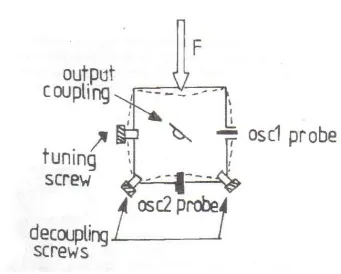
Figure 2.1: Conceptual layout of cavity with two orthogonal resonators - reproduced from

(30)

One of the assumptions is that the two oscillators are decoupled, and this is unlikely

when they are both running in the same cavity. The authors talk about this issue and

detail tuning screws for decoupling and the need for finely adjusting the screws and

oscillator probe lengths.

The method of loading the cavity causes non-linear bulging of the cavity walls as shown

in fig. 2.2, and this is likely to cause non-linearity between the applied load and change

in output frequency. They claim good linearity but only detail this up to a modest 10

kg load.

Figure 2.2: View of the Farley et al. (1991) cavity cross section under load - reproduced

from Fig 5.

Finally, the oscillators are an old negative resistance type. This method had its

(31)

2.3 Force Measurement and Transduction Options 10

field effect transistor oscillators. While they were adequate and relevant at the time,

and may still find some application in low cost devices, there are better options available

now.

This project aims to incorporate the better features of the Farley et al. (1991) design,

and improve on some of the disadvantages. It is also a goal to use modern electronics

for the oscillators and signal processing blocks.

2.3

Force Measurement and Transduction Options

With the exception of direct weight comparison devices like balance scales, the majority

of force or weight transducers depend on the elastic deformation of a mechanical element

within the linear boundaries of Hooke’s law, with some device to measure the strain or

displacement in the mechanical member.

2.3.1 Strain Gauges

The electrical strain gauge is a transducer that changes its resistance when it is strained

by displacement (Mackay 1994). The basic concept is that a strain gauge being

length-ened by strain in the member it is bonded to, causes the cross-sectional area of the

conducting elements in the gauge to reduce, hence increasing the resistance of the

gauge. The converse argument can be made for a strain gauge being compressed. The

formula used is Equ 2.1.

R=ρLo

A (2.1)

where:

R is the resistance in Ω ρ is the resistivity in Ω.m Lo is the length in m

(32)

In strain gauges the fractional change in resistance is more important than the total

resistance of the gauge. The gauge resistance is important to set the d.c. operating

point, but the strain data is contained in the fractional change of resistance, which is

defined by Equ. 2.2.

∆R Ro

= (1 + 2σ)∆L L0

+∆ρ

ρ (2.2)

where:

∆R

Ro is the fractional change in resistance σ is Poisson’s ratio

∆L

Lo is the fractional change in length ∆ρ

ρ is the fractional change in resistivity

From this the gauge factor of the strain gauge can be deduced, and is shown in equ.

2.3. GF = ∆R Ro ∆L Lo

= 1 + 2σ+ ∆ρ

ρ

∆L L

(2.3)

A strain gauge is designed to respond to change in its length, however expansion and

contraction of the elastic member the gauge is bonded to will cause the gauge to change

length. Thus a single strain gauge is an effective strain sensor, and an equally effective

temperature sensor. A method has to be devised to discriminate the effects of

temper-ature change. The usual method is to use at least two strain gauges in a wheatstone

bridge arrangement, where a loaded elastic member will cause one gauge to be stretched

and the other to be compressed. When the gauges are correctly placed in the bridge the

output due to load will be doubled. However temperature change causes both gauges

to be equally changed in length, and this is cancelled in the bridge circuit. High quality

strain gauge systems usually use four strain gauges, with one gauge in each leg of the

bridge.

The most common form of strain gauge is the foil type. The gauge consists of an

(33)

backing. Most modern foil strain gauges also have a protective plastic layer bonded

over the top surface of the gauge. When strain occurs in the mechanical member that

the gauge is bonded to, then the fine foil traces along the length of the gauge are

either stretched or compressed. When a foil trace is stretched its cross-sectional area

is reduced and it electrical resistance increases, with the opposite happening when the

trace is compressed - as per Equ. 2.1. Gauges are usually arranged so mechanical strain

is arranged along the length of the foil traces, with short end connections between the

traces providing reduced sensitivity to strain in other directions. The gauge is then

bonded to the mechanical elastic member using special glues, and it is particularly

important that there is no creep in the glue line, otherwise the system will gradually

drift off zero. Creep in the glue line will allow long term relative movement between the

gauge and the mechanical member, and this movement is what causes the zero offset.

This is a particular problem if a static load is applied to the elastic member for a long

period of time. To achieve a glue line of this quality involves a costly and complex

surface preparation and glue curing procedure. Poor control of these procedures will

lead to a high production defect rate, and premature failure of products.

Strain gauge based wheatstone bridge circuits have a very low level differential signal

sitting on a high level common mode voltage. This requires a specialised analogue

circuit to amplify the differential signal whilst providing a high common mode rejection

ratio (CMRR). These systems are very prone to moisture and temperature changes,

and require special consideration of these issues to maintain sufficient stability. Modern

electronics is rapidly moving toward system on a chip technology, where minimization

of analogue circuitry is an advantage. Strain gauges are still a viable technology, but

no longer match modern circuit techniques quite so well anymore.

2.3.2 Mechanical Resonant Systems

The most basic mechanical resonant system includes a long steel wire attached to the

side of the elastic load bearing member in such manner that the tension in the wire

changes as the elastic member strains. The steel wire is also electrically insulated from

the elastic member, and is coerced into resonant oscillation by placing a permanent

(34)

The magnetic field induced around the wire by the alternating current couples with the

magnetic field from the permanent magnet, and provides an alternating force on the

wire. When the frequency of the alternating current is close to the resonant frequency of

the wire, the amplitude of the oscillation in the wire increases. The resonant frequency

is related to the tension in the wire by the well known equation 2.4 (Halliday & Resnick

1977).

fn=

1 λn

v = n 2L

s

T

µ (2.4)

Where:

L = length of wire ( m)

T = tension of wire (N)

µ= wire mass per unit length (kg/m) v = wave propogation speed (m/s)

λ= wavelength (m)

fn = resonant frequency (Hz)

A more developed version of this concept is described by Yan et al. (2003) where thin

stainless steel resonantors are made, with piezo-electric drivers and detectors screen

printed onto the resonator. The triple beam tuning fork resonator consists of a

stain-less steel device 15.5 mm long, 0.25 mm thick, 2 mm wide centre beam and two 1

mm wide outer beams. A feedback closed-loop circuit can maintain the resonator in

resonance while loads are applied to the resonator, resulting in changes in its resonant

frequency. The circuit outputs a digital frequency signal for measurement, which

inte-grates very well with modern circuit techniques. Unlike strain gauge systems, no costly

and sensitive analogue circuitry is required. The designers also claim a higher overload

capability than strain gauge based systems.

The authors used an epoxy-phenolic adhesive to attach the resonators to the elastic

member, but later note that a bolted system would be better. The resonator would

also be suitable for resistance welding to the elastic member, providing an even more

(35)

Some of the issues with this design include the effects of mechanical impacts and

vi-bration disturbing the resonant mode of the resonator, and that the resonator must

operate in free space so potting for environmental sealing is not an option.

2.3.3 Hydraulic Systems

Hydraulic force measurement systems have existed for a long time, and involve

apply-ing the force to be measured to a piston or diaphragm and monitorapply-ing the pressure

produced. The pressure generated will equal the force divided by the area of the piston

or diaphragm, less frictional or flexural forces in the system. Nothing is really gained

with these systems as some method of measuring the pressure is still required, and the

hydraulic circuitry is a source of additional errors. The notable exception may be when

a hydraulic circuit already exists and precise measurement is not required. Some

card-board baler controllers utilise a hydraulic pressure switch that has a set point pressure

at which the switch contacts change over. This switch changeover is used to indicate

the bale of cardboard is full, based on the simple concept that the baler has supplied

its maximum designed force onto the bale and has not driven the pressing apparatus

to the bottom of its movement stroke as detected by a limit switch.

2.3.4 Fibre Optic Systems

Optical fibre sensors offer many advantages including immunity to electromagnetic

interference and the ability to locate sensitive electronic equipment away from shock,

temperature variations and other environmental disturbances (Vaziri & Chen 1991). If

sensitivity is the main consideration then optical interferometric sensors have no equal,

whereas multimode fibre sensors with LED light sources and p-i-n diode detectors are

preferred if simplicity and robustness are important.

The basic principle is to perturb the optic fibre in some way so as to alter its light

transmission characteristics. Many methods have been developed to perturb the fibre,

including gauge heads designed to convert longitudinal and/or transverse stress to fibre

(36)

2.4 MMIC based Oscillators 15

1982), and a roller chain like device with the fibre threaded through the chain (Mavin

& Ives 1984). Many other variations exist including microbend sensors in which threads

are wound around the glass fibre, and tactile sensors in which force is converted to fibre

deformation.

Many of the issues with drift and hysteresis in multi-mode fibre strain sensing systems

can be traced to the structure used to perturb the fibre. Etched fibres have been

developed to try to minimise these effects (Vaziri & Chen 1991).

2.4

MMIC based Oscillators

The GaAs (gallium arsenide) MESFET (metal-semiconductor field effect transistor) was

the first practical device suitable for MMIC (monolithic microwave integrated circuit)

applications, and was investigated by Mead (1966) and Hooper & Lehrer (1967). The

first practical MMIC devices were used by the US military in the early 1970’s as low

noise amplifiers for military and space applications. Fairchild released a device with

11dB gain at 8 GHz in 1976 (Bechtel 2003). Current devices use technology like InGaP

but retain the basic characteristics of the earlier devices. The defining advantages of

MMICs are their ruggedness and the uniformity of devices which eliminates the need

for trimming or adjustment of circuits. They are also relatively low cost and suited to

modern automated assembly processes.

There have been a wide variety of cavity oscillators used, with negative resistance

de-vices being the most common. Section 2.5 talks at some length about the design process

for this type of resonator, so in this section MMIC based loop feedback resonators will

be focused on.

Resonators based on MMIC amplifiers are feedback oscillators with two coupling ports

into the cavity (Barth 2000). They depend on 360 electrical degrees of phase shift

be-tween the two coupling ports, and sufficient gain in the MMIC amplifier to compensate

for weak coupling to the cavity. This oscillator configuration requires a loop analysis

(37)

Figure 2.3: Setup of the Barth (2000) feedback oscillator clearly showing the two coupling

(38)

Leeson’s Equation (Leeson 1966) describes the phase noise in the 1/f2 region, and is reproduced in Equ. 2.5.

L(∆ω) = 10log(2kT F Ps

( ω

2Q∆ω)

2₎ _(2.5)

where:

L(∆ω) = phase noise (dbc/Hz) k=Boltzman’s constant (J/K) T = temperature (K)

F = device’s noise factor (dBc/Hz) Ps=power in resonator (W)

∆ω =offset frEquency (rad/s) ω=angular frEquency (rad/s) Q=resonator loaded quality factor

Because low phase noise will lead to a spectrally purer signal to monitor cavity strain,

then the aim is to reduce the numerator and/or increase the denominator in Equ. 2.5.

By inspection it can be seen that increasingPs orQwill reduce phase noise. However

doublingPsreduces phase noise by 3dB whilst doublingQreduces phase noise by 6dB.

The two main sources of loss in the cavity are dielectric loss and metallic loss due to

finite surface conductivity. If the dielectric is air then the loss is negligible. Any high

conductivity metal will give reasonable Q factors, and silver plating the inside of the cavity will also increase conductivity.

Barth (2000) states ”a gain as high as possible allows weak coupling to the resonator

resulting in doubling the Q-Factor or improving the phase noise by nearly 6dB”. So

a high gain in the feedback amplifier allows weak coupling to the cavity, and hence

(39)

2.5 Prior Methods of Realising a Cavity Oscillator 18

compensate for weak coupling to the cavity and other losses in phase shift devices.

The volume of work on cavity oscillators seems to decline before the availability of

suitable low cost MMIC devices, due to the industry shifting towards dielectric resonant

oscillators, because they are smaller in size, cost and weight than equivalent metal

cavities, and can be very easily incorporated into microwave integrated circuits and

coupled to planar transmission lines (Pozar 2005). With the continued development

of high frequency devices that can directly operate in the microwave bands, many

direct frequency generation methods have been devised, especially for mobile devices

like phones. These direct frequency generation methods allow greater device flexibility

like frequency hopping.

In recent years there has been a renewed interest in cavity resonators, in an attempt to

improve the spectral purity of oscillators. The limitation of a high spectral purity

on-chip oscillator is the integrated resonator, and Khalil et al. (2011) describes a method

to integrate a cavity resonator onto a GaAs MMIC chip.

There is sufficient work done in this area of loop feedback MMIC cavity resonators to

indicate the viability of the system for this application.

2.5

Prior Methods of Realising a Cavity Oscillator

The following sub-sections detail some of the considerations in designing a cavity

oscil-lator using junction transistors or field effect transistors.

2.5.1 Oscillator Theory

According to Hodowanec (1974), at microwave frequencies, the most effective transistor

configuration for an amplifier is the base mode of operation. The

common-base configuration provides higher gain, efficiency, and stability at frequencies above

the transistors fT than any other configuration. Oscillators are a form of regenerative

(40)

Figure 2.4: Oscillator Equivalent Circuit : partly reproduced from Materka & Mizushina

(1982)

common-base oscillator is the Colpitts circuit (Millman 1979, p653), because it makes

use of a tapped capacitor circuit to provide the correct feedback. Often part of this

capacitance network can be provided by parasitic package capacitance of the transistor.

Materka & Mizushina (1982) have shown that a cavity oscillator can be constructed

using stripline circuitry that is frequency locked to the cavity resonant frequency via

probe coupling. They have used a coaxial transformer to match the active device

admittance to the admittance of the cavity and probe coupling mechanism.

Materka & Mizushina (1982) work also involved an inductive window in the cavity to

couple multiple oscillators. By deleting this feature and using their equivalent circuit,

the circuit shown in Fig. 2.4 was drawn, where the active device is represented by Yd

whose admittance YD(A, f) has its real part negative in a certain frequency range,

where A is the amplitude of RF voltage across the device terminals at frequency f. The LCR parallel circuit represents the cavity. Xp is the probe reactance and the

ideal transformer (n1: 1) represents the probe coupling. Zt denotes the characteristic

impedance of the coaxial transformer whose length is lt.

Materka & Mizushina (1982) also used the well known condition for sustained steady

(41)

seen from port a-a’ (Fig. 2.4) looking toward the cavity:

−YD(Ao, fo) =YL(fo) (2.6)

whereAo and fo are respectively the amplitude and frequency of oscillation.

2.5.2 Impedance Transformers

However, the coaxial transformer described by Materka & Mizushina (1982) is a three

dimensional mechanical structure not well suited to modern microwave stripline

con-struction methods. A stripline impedance transformer would have considerable

manu-facturing benefits. Womack (1962) in his paper titled ”‘The Use of Exponential

Trans-mission Lines in Microwave Components”’ describes a tapered line section suitable for

making this transformation. Tapered line sections can perform similar transformations

to standard stripline impedance transformers, but at reduced size.

According to Womack (1962) a tapered line is defined by:

Ko(x) =Ko1e(δx) (2.7)

Where Ko1 is the impedance at x = 0, and δ is the rate of taper. There are two conditions in which impedance transformers are applied - see Fig. 2.5.

For Fig. 2.5 (a) where ZL

Ko2 >>1 then

Zs

Ko2

= jX(ω) Ko2

+ Z¯ Ko2

(2.8)

WhereX(ω) =Ko2F(ω) and

¯

Z = Ko1Ko2 ZL

(42)

Figure 2.5: Tapered Stripline Transformers reproduced from Womack (1962)

and for Fig. 2.5 (b) whereZL<< Ko1 then

Zs

Ko1

= 1

jKo1B(ω) +Ko1Y¯

(2.10)

where ¯Y = ZL

Ko1Ko2 and

B(ω) = F(ω) Ko1

(2.11)

F(ω) can be obtained in the graphs in Fig. 2.6, where βo= 2_λπ.

Also the minimum length of the line was calculated using equ 2.12.

lo= λ

2

1− δ2

4β2 1₂

(2.12)

Select |δ_β| between 0 and 2. The larger _βδ the shorter the line.

(43)

Figure 2.6: Variation ofF(ω) with frequency for various values of the ratio _βδ

o reproduced

(44)

Figure 2.7: Two-port transistor oscillator circuit - reproduced from Kai Chang & Nair

(2000)

slight increase in length.

2.5.3 Criteria for Cavity Oscillation

Referring to Fig. 2.7 and Kai Chang & Nair (2000) - the terminating network is used to

provide|Γout|>1 (or Rout<1), which is a necessary condition for oscillation to start.

The load network incorporates the probe and cavity, and determines the oscillation

frequency.

Using transistor S-parameters the stability factor of the device is calculated from equ

2.13.

K = 1− |S11| 2_{− |}_S

22|2+|S11S22−S12S21|2 2|S12S21|

(2.13)

and will be less than 1 for potentially unstable devices. The conditions for oscillation

were expressed as:

(45)

ΓinΓT = 1 (2.15)

ΓoutΓL= 1 (2.16)

or expressed another way:

|Rout(V, fo)|> RL(fo) (2.17)

Xout(V, fo) +XL(fo) = 0 (2.18)

whereRout is a negative resistance.

According to Kai Chang & Nair (2000) the following basic steps can be followed to

design a transistor oscillator :

• Select a potentially unstable transistor at the frequency of oscillation, or use

feedback elements to make it unstable.

• Design the terminating network,ZT or ΓT, to make|Γout|>1 by choosing ΓT or

ZT in the unstable zone of the stability circle.

• FromZT and the transistor small signal S-parameters, calculate Γout and confirm

|Γout|>1.

Γout=S22+

S12S21ΓT

1−S22ΓT

(2.19)

|Γout|>1 (2.20)

• Choose the load according to the oscillation condition as follows:

XL(fo) =−Xout(fo) (2.21)

RL(fo) =

1

(46)

The chosen value for ZL usually produces a working oscillator. The measured

oscillation frequency will be shifted from the design value, since Xout(fo), used

in determiningfo, is assumed to be independent of the amplitude V.

• Design the load matching network to transform a 50Ω load toZL.

The output load in this design will be the circuit to find the difference frequency between

the two cavity oscillators. The impedance was selected to be the industry standard 50Ω.

The negative resistance Rout is a function of voltage and as the oscillation power is

increased, the negative resistance value reduces. If the negative resistance value reduces

to a value below the load resistance, oscillation ceases. To overcome this problem the

magnitude of the negative resistance at V = 0 was designed to be much larger than the load usingRL(fo) = 1₃|Rout(0, fo)|.

Stability circles were plotted on a Smith chart to indicate areas whereK <1 (Bowick 1997). The perimeter of the circle represents a locus of points whereK = 1, and either the inside or the outside of the circle can represent the unstable region. The following

was used to calculate the stability circle:

Ds=S11S22−S12S21 (2.23)

C1 =S11−DsS22∗ (2.24)

C2=S22−(DsS11∗ ) (2.25)

The centre of the input stability circle was calculated using:

rs1 =

C₁∗

|S11|2_{− |}_D

s|2

(47)

and the radius of the input stability circle was calculated using:

ps1 =|

S12S21

|S11|2− |Ds|2

| (2.27)

The centre location of the output stability circle was calculated using:

rs2 =

C₂∗

|S22|2− |Ds|2

(2.28)

And finally, the radius of the output stability circle was calculated using:

ps2 =|

S12S21

|S22|2− |Ds|2

| (2.29)

Using this data the stability circles were then plotted on a Smith chart. In most cases

transistors are stable at 50Ω, so S11 and S22 will be less than 1. S11 and S22 would be greater than 1 for an unstable transistor. The centre of the normalised Smith chart

must be part of the stable region, and if the stability circle surrounds the centre of the

Smith chart, then the inside of the circle is the stable region. Alternatively, if the circle

does not surround the center of the chart, the entire area outside the circle represents

(48)

Chapter 3

Initial Design Concepts and

Microwave Cavity Measurements

3.1

Introduction

This chapter outlines the some of the formative thought processes and investigation that

ultimately led to the outcomes detailed in future chapters. The first half of the chapter

covers some of the design iterations in regard to the mechanically loaded member, and

the second half investigates prior methods of realising and designing cavity oscillators.

3.2

Mechanical Designs

Several options for mechanical designs have been investigated in an attempt to find

a method of producing predictable and geometrically simple deformation in a loaded

cavity within a cantilever beam. Initially investigation focused on options where one

cavity would be compressed and the other expanded in structures like the beam shown

in Fig.3.1, thus giving maximum frequency shift for a given load. However no

solu-tion was found that did not produce complex cavity deformasolu-tions. Several versions

of beam design were drawn on 3 dimensional computer aided drafting package (Alibre

(49)

3.2 Mechanical Designs 28

Figure 3.1: Simple Cantilever Beam

(ALGOR Design Check - version 23.1). One of the later variants is shown in Fig.3.2,

however they all produced complex deformation of the cavities.

In an attempt to produce cavity deformation that allowed the cavity to remain close to

square with relatively straight sides, strain control holes were investigated. A variant

of this design is shown in Fig. 3.3 and some displacement data from analysis is shown

in Fig. 3.4. While this does to some degree make the deformation of the cavities more

geometrically simple, it also localizes most of the strain into the strain control holes

which is undesirable.

A beam was then devised that would bow in the center by having two support points

at either end, and two load points at either end but displaced from the support points.

(50)

(51)

(52)

Figure

3.4:

Displacemen

t

of

Beam

with

Strain

Con

trol

Holes.

The

colour

bar

sh

o

ws

displacemen

t

in

(53)

3.3 Investigation of Cavity Coupled Microwave Oscillators 32

and the upper cavity is compressed. The curvature introduced into the cavity is in

the co-ordinate direction in which there is no resonant mode (see Chapter 5: sections

5.3 to 5.5), so this would possibly not effect the performance electrically. However this

arrangement is difficult to provide with electrical coupling devices located in a single

coplanar printed circuit board.

A block was then devised that was designed to be subjected to compression loads. This

design is shown in Fig. 3.6 and a series of automatically generated images of stress,

strain and deformation from finite element analysis simulation results are shown in Fig.

3.7. The block dimensions were selected in an intuitive manner starting with the cavity

dimensions of 40 x 40 mm, as this gave manageable resonant frequencies. If this design

was further investigated then dimensional data would have been selected in a more

formal manner, with a focus on achieving certain strain to load ratios. Mechanically

this again exhibited properties that provided measurement cavity deformation mainly

in one co-ordinate direction with the general shape of the cavity remaining rectangular,

but was also difficult to make electrical couplings to the cavities from a single printed

circuit board.

3.3

Investigation of Cavity Coupled Microwave

Oscilla-tors

A lot of work was done to investigate the merits of prior art technology for the current

project. While most of this was ultimately rejected as being unsuitable, this did provide

valuable background information and is detailed in Chapter 2: Section 2.5. The final

decision was to try and use MMIC technology which did not exist when most of the

concepts in Chapter 2 were current. MMIC technology is available in surface mount

packages, is well adapted to modern assembly methods and is readily available at low

(54)

Figure

3.5:

Displacemen

t

of

Bending

T

yp

e

Beam

under

(55)

(56)

(57)

3.4 Impedance of a trial Cavity and Probe 36

3.4

Impedance of a trial Cavity and Probe

A pair of 40 mm by 40 mm by 10 mm cavities were machined in a 6061T6 Aluminium

beam, as shown in figure 3.8. This design is the equivalent of that shown in Fig. 3.5.

A probe as shown in Fig. 3.9, is mounted in a plate as shown in Fig. 3.10. The plate

assembly is then mounted to the aluminium beam to close the cavities, as shown in

Fig. 3.11.

The cavity was then scanned over a range of frequencies from 5.1 GHz to 5.3 GHz using

an HP8720 Network Analyser, and a data file of frequency verses complex reflection

coefficients were obtained. Two different probes were used with tip lengths of 3 mm

and 5 mm, with data being recorded for both.

The reflection coefficient must be converted to a complex impedance at each frequency

point. This conversion was computed using Matlab. The reflection coefficient is

de-scribed in equ 3.1.

Γ = ZL−Zo ZL+Zo

(3.1)

By rearranging this can be converted to equ 3.2.

ZL=Zo

1 + Γ

1−Γ (3.2)

The network analyser is a standard load, so assume Zo = 50 Ω. The results of this

(58)

Figure 3.8: Picture of Cavities

(59)

Figure 3.10: Picture of the Probe and Cavity Cover Plate Assembly

(60)

Figure 3.12: Comparison between Impedance Phase and Magnitude for 40 mm Cavity with

(61)

Figure 3.13: Comparison between Impedance Phase and Magnitude for 40 mm Cavity with

(62)

Chapter 4

Mechanical Design of Transducer

4.1

Introduction

This chapter outlines the important characteristics of cavity strain in this

applica-tion, and continues on to investigate important properties of the mechanical member.

Physical properties of the mechanical member like the relationship between Young’s

modulus and temperature, stress concentration, fatigue, creep, corrosion and electrical

properties are considered. The preferred mechanical design is introduced, and strain

calculations are outlined.

4.2

Cavity Geometry

A large variety of geometrical shapes and many more random shapes can function as a

resonant cavity, however performance of the cavity is difficult to define mathematically

if anything other than simple geometric shapes are used. Further, it is usually easier

to machine simple geometric shapes, and maintain accuracy and repeatability. So this

limits the set of choices for cavity shape to rectangular, square, cylindrical and spherical.

Due to machining difficulty spherical shapes were immediately abandoned, and square

shapes are simply a subset of rectangles. To control the higher order resonance modes,

(63)

4.2 Cavity Geometry 42

In this application it is important to have a well defined mechanical relationship between

cavity strain and applied load. It is also desirable to have this strain act totally in one

co-ordinate direction, which provides a simple relationship between applied load and

cavity resonant frequency. It would be difficult to machine a cylindrical hole into a

loaded member and have this well defined strain to load relationship if the cylinder was

strained in a radial direction. A cylindrical hole will tend to elongate in one co-ordinate

direction, and pull inward in an orthogonal co-ordinate direction producing a complex

deformation of the cylindrical hole. This in turn produces a complex relationship

between cavity resonant frequency and applied load. For a rectangular cavity the

resonant frequencies are given by Pozar (2005) as:

fm,n,l= (

c 2π√µrr

)

r

(mπ a )

2_{+ (}nπ b )

2_{+ (}lπ d)

2 _(4.1)

where:

fm,n,l= cavity frequency for mode m, n, l

µr= relative permeability of material filling cavity

r = relative permittivity of material filling cavity

m, n, l= number of variations in standing wave pattern inx, y, z directions a, b, d= cavity dimensions inx, y, z directions

c= velocity of light in free space

See Fig. 5.1 for a graphical representation of the variables in Equ. 4.1.

4.2.1 Cylindrical Cavities

It is possible to strain a cylindrical hole in its axial direction and achieve good linearity.

Hylarides bridge configuration (Carlton 2007) is an example of a strain gauge based

system that uses axial strain in a cylinder or shaft as the basis of a transducer

mechan-ical element. However as covered in the chapter on Microwave Resonator Theory, a

(64)

4.2.2 Square Cavities

If a square cavity is used, then it can be designed with two thin web walls co-planar

with the direction of applied load, and with the load applied so the web walls are

under tension. This provides a mechanical arrangement where the cavity dimensions

mainly change only in one co-ordinate direction, with little change in other directions.

A design of a cavity using this principle is shown in Fig. 4.1. To prove the validity of

this concept the design was constrained in a finite element analysis package as shown

in Fig. 4.2, with the triangles on the two abutments being where the transducer would

be rigidly bolted to a support structure and would represent full movement constraint

at these faces, and the applied load is represented by the series of six green arrows at

one end of the structure. Finite element analysis was performed on this with a load of

1000 N and the strain results are shown in Fig. 4.3.

From Fig. 4.3 three very important observations were made:

Firstly, the reference cavity at the end most distant from the applied load is virtually

unstrained, which means its frequency of resonance will not alter significantly as load

is applied. However this cavity shares a common temperature profile with the

mea-surement cavity and can be used to compensate for ambient temperature variation.

Second, the arrow head shaped block that the load is applied to has shown some

strain due to the lighter shading, but this strain is very nearly uniform as indicated

by the constant shading colour across the section. This indicated that the face of the

measurement cavity closest to the applied load must be remaining very close to straight.

Also the measurement cavity face farthest from the applied load also must be remaining

straight due to the absence of strain in the web between the measurement and reference

cavities. This indicated that a simple one dimensional change of cavity shape due to

applied loads is very nearly achieved, making the analysis of cavity resonant frequency

change verses applied load very simple.

Lastly, it can be seen that all the strain is concentrated in the side webs of the

mea-surement cavity, and that this strain is uniformly distributed along the length of the

(65)

mechanical failure. The inside corners of the cavities have a fillet curve which also

helps reduce stress concentration, and naturally allows a rotating mill tool to cut out

the cavity.

The assumption made is that the fields in the corners are small and the corner radii

have a negligible effect on the cavity resonant frequency. These corner radii can be

considered to be cavity perturbations, and Pozar (2005) has a Section 6.7 ”Cavity

Perturbations” with a Subsection titled ”Shape Perturbations”. This section details a

method to calculate the change in resonant frequency due to small changes in cavity

shape. The method works on the idea that the amount of stored magnetic or electric

field is altered by the cavity perturbation. Pozar (2005) developed Equ. 4.2.

ω−ωo

ωo

= ∆Wm−∆We Wm+We

(4.2)

where:

ω= perturbed cavity resonant frequency ωo=original cavity resonant frequency

∆Wm= change in stored magnetic field energy

∆We=change in stored electric field energy

Wm = original stored magnetic field energy

We= original stored electric field energy

The perturbation method predicts a frequency shift due to the corner rounding in the

right direction, but only slightly more than half that measured. There are some doubts

associated with this calculation as the size of the corner radius probably exceeds the

definition of ’small changes in cavity shape’.

From Section 5.5 the calculated resonant frequency is:

f2,1,0 = 8.3794 GHz

(66)

4.3 Choice of Materials for the Mechanical Element 45

f2,1,0 = 8.2675 GHz

This is a difference of 0.1119 GHz or 1.33 % of the calculated resonant frequency. Some

of this discrepancy is certainly due to machining imperfections (run-out, taper and

machining marks) as the cavities were made on a basic hand operated milling machine.

It was observed that the location and length of the coupling probes also seemed to

slightly alter the resonant frequency, and the frequency shift due to coupling pro

Measuring strain using microwave energy

University of Southern Queensland

Certification of Dissertation

ENDORSEMENT

Acknowledgments

Contents

List of Figures

List of Tables

Chapter 1

Hypothesis

Research Aims and Objectives

Structure of the Dissertation

Chapter 2

Measuring Mechanical Strain using a Cavity Resonator

Force Measurement and Transduction Options

MMIC based Oscillators

Prior Methods of Realising a Cavity Oscillator

Chapter 3

Mechanical Designs

Investigation of Cavity Coupled Microwave

Impedance of a trial Cavity and Probe

Chapter 4

Cavity Geometry