Generalized phase-space kinetic and diffusion equations for classical and dispersive transport

This content has been downloaded from IOPscience. Please scroll down to see the full text.

Download details:

This content was downloaded by: bronsonphilippa IP Address: 137.219.57.159

This content was downloaded on 28/07/2014 at 22:40

Please note that terms and conditions apply.

Generalized phase-space kinetic and diffusion equations for classical and dispersive transport

View the table of contents for this issue, or go to the journal homepage for more 2014 New J. Phys. 16 073040

equations for classical and dispersive transport

Bronson Philippa, R E Robson and R D White

ARC Centre for Antimatter-Matter Studies, School of Engineering and Physical Sciences, James Cook University, Townsville 4810, Australia

E-mail:[email protected]

Received 10 April 2014, revised 16 May 2014 Accepted for publication 6 June 2014

Published 28 July 2014

New Journal of Physics16(2014) 073040 doi:10.1088/1367-2630/16/7/073040

Abstract

We formulate and solve a physically-based, phase space kinetic equation for transport in the presence of trapping. Trapping is incorporated through a waiting time distribution function. From the phase-space analysis, we obtain a gen-eralized diffusion equation in configuration space. We analyse the impact of the waiting time distribution, and give examples that lead to dispersive or non-dispersive transport. With an appropriate choice of the waiting time distribution, our model is related to fractional diffusion in the sense that fractional equations can be obtained in the limit of long times. Finally, we demonstrate the appli-cation of this theory to disordered semiconductors.

Keywords: kinetic theory, dispersive transport, fractional diffusion equation

1. Introduction

The link between theory and experiments measuring transport properties in either gases or condensed matter is provided by an advection–diffusion equation or Fokker–Planck equation for number density n( , )r t [1]. These configuration-space theories are only valid in the hydrodynamic regime of smooth spatial gradients [2]. It is therefore fortunate that physical systems such as crystalline condensed matter and gaseous media rapidly approach this regime. In these systems, collisions are effectively instantaneous, and memory of the initial condition is lost after only a few collisions. Any large gradients are quickly smoothed. For such‘classical’

transport, the corresponding diffusion equation is a conventional partial differential equation of first order in t and second order in r. Such systems are characterized by a diffusive regime wherein the mean square displacement grows linearly, i.e.

〈 〉

x2 − x 2 ∼ t. In contrast, there is an increasing body of literature demonstrating‘anomalous’diffusion, wherein the mean square displacement is nonlinear, i.e.

〈 〉

x2 − x 2 ∼ tγ where γ ≠ 1 [3]. To mention just a few, subdiffusion (γ < 1) occurs in the transport of charge carriers in disordered semiconductors [4, 5], and the movement of lipids and proteins of cell membranes [6]; whereas Lévy flight (γ > 1) has been observed in the diffusion of ultracold atoms in an optical lattice [7, 8].

Subdiffusion is fundamentally slower than regular Brownian diffusion. It arises from repeated trapping and de-trapping of the transported species, in which periods of ‘classical’ transport are interrupted by (potentially long) periods of immobilization. Consequently, the memory of the initial condition may persist for long times, and large gradients are not necessarily smoothed out. Such effects are often accounted for by replacing the conventional time derivative with a fractional derivative [9–13], which in turn accounts for the memory effects. However, the spatial gradient terms are left intact, and thus the weak gradient assumption is therefore still implicit. This is an apparent contradiction that challenges the validity of the fractional diffusion equations. Until now, this issue has only been addressed in an ad hoc matter, through solution of an exactly solvable model kinetic equation in phase space [14]. The phase space system does not require the assumption of weak gradients, so this questionable assumption is avoided. Trapping effects were incorporated in the ‘collision term’ in a way which, although consistent with other contemporary kinetic equations, is nevertheless ad hoc in nature, and therefore warrants further scrutiny [14].

This paper resolves the ad hoc nature of the previous approach by revisiting the phase space formulation. We develop from first principles a new physically-based, exactly solvable model kinetic equation, whose solution leads, in the weak gradient limit, to a generalized diffusion equation. This equation provides a general description of transport in the presence of trapping. In the appropriate limit of instantaneous de-trapping, it reduces to the classical diffusion equation. Conversely, in the case of traps that possess a divergent waiting time, dispersive (subdiffusive) transport is obtained, similarly to the fractional diffusion equations commonly studied [15–18].

2. Procedure

Kinetic theory aims at finding the charge carrier phase space distribution function f ( , , ),r v t

3. The phase space model

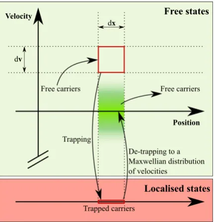
Figure1outlines the phase space trapping and de-trapping picture schematically. Suppose that at time t charge carriers moving freely are scattered out of a phase space element centred on

r v

( , ) at a constant rate ν into localized or trapped states, i.e., the rate of loss is -νf ( , , ).r v t

They remain trapped for a range of various possible timesτ, as determined by the waiting time distribution, defined such that ϕ τ( ) dτ is the probability of de-trapping between times τ and τ + dτ after the trapping event. Thus the rate at which particles are re-entering the phase-space element under consideration at time t isν

∫

tdτϕ τ( ) f ( , ,r v t − τ) ≡ ν

0 detrap ϕ*fdetrap, where ⎛

⎝

⎜ ⎞

⎠

⎟ ⎛

⎝ ⎜ ⎜

⎞

⎠ ⎟ ⎟ π

= −

f t n t m

k T

m

k T

r v r v

( , , ) ( , )

2 _B exp 2 _B (1)

detrap

3 2 2

is the distribution function for the de-trapped particles, assumed to be a Maxwellian at medium temperature T. Here, m is the particle mass (or effective mass), and k_B is the Boltzmann constant. The corresponding free particle function is thus

 ν⎡_⎣ ϕ ⎤_⎦

∂ + · + · ∂ = − − *

(

_t v a _v

)

f f f , (2)

detrap

[image:4.595.144.361.121.345.2]

wherea is the external force per unit mass. Note that only thesecond(de-trapping) term on the right hand side is convolved with ϕ, corresponding to a delayed release from the localized states. In contrast, scattering into traps takes place without any delay, and thefirstterm on the right hand side isnotconvolved. We note that the classical BGK equation [20], well known in gas and crystalline semiconductor transport studies, is regained when collisions are instantaneous. Instantaneous collisions are recovered by setting the waiting time distribution to be the Dirac delta, i.e.ϕ τ( ) = δ τ( ).

We now define the operator

ν ϕ

∂ ≡ ∂ +∼_{t t} [1 − *], (3)

and write equation (2) in the equivalent form

 νϕ ⎡_⎣ ⎤_⎦

∂ + · + · ∂ = − * −

∼

(

_t v a _v

)

f f f . (4)

detrap

Integration of (4) over all velocities yields the equation of continuity,

 Γ

∂∼_t n + · = 0, (5)

where Γ =

∫

d3v v f ( , , )r v t is the free particle flux. A further integration over r yields

∂∼_tN = 0, (6)

where N t( ) =

∫

d r d v f3 3 ( , , )r v t is the total free particle number. Since this implies

ν ϕ

∂_tN = − [1 − *]N ≠ 0, it is clear that the number of free carriers is not constant in time, unless eitherν → 0 or ϕ( )t →δ( )t .

The solution of equation (2) in infinite space, with the initial condition, ⎛ ⎝ ⎜ ⎞ ⎠ ⎟ ⎛ ⎝ ⎜ ⎜ ⎞ ⎠ ⎟ ⎟ δ π = −

f N m

k T

m

k T

r v r v

( , , 0) (0) ( )

2 _{B 0} exp 2 _B (7)

3 2 2

0

corresponding to release of N (0) particles from the origin of coordinates with a Maxwellian distribution of velocities with an initial temperatureT₀, can be obtained exactly through Fourier and Laplace transformation in space and time respectively, following the same mathematical procedure as [14] and [21]. The transformed number density then follows

⎡⎣ ⎤⎦

∫

∫

ξ ν ξ

νϕ ξ ν ξ

= − · −

= − +

− ˆ − +

−∞

∞ ∞

( )

( )

n p i t pt n t

N T Z p T

p T Z p T

k r k r r

( , ) d exp ( ) d exp ( ) ( , )

(0) ( )

1 ( ) ( ) [ ( ) ( )], (8)

0

0 0

wherek is the Fourier variable, p is the Laplace variable, ⎛

⎝

⎜⎜ ⎞_⎠⎟⎟

ξ = + ·

− T i k T m i k a k k

( ) 1

2 , (9)

B

2 1 2

·

Z[ ] is the plasma dispersion function defined by Z( )ζ = i πe−ζ2 erfc (−iζ), and

∫

ϕ^( )p = ∞d exp (t −pt) ϕ( )t

0 is the Laplace transform of the waiting time distribution.

Inversion of the Laplace transform of equation (8) could be carried out, if desired, through the usual contour integral, which would be evaluated using the residue theorem in terms of the singularities ofn p( , )k , which are given by the zeroes of the denominator of (8), i.e.,

νϕ ξ ν ξ

− ˆ p T Z − p + T =

1 ( ) ( ) [ ( ) ( ) ] 0. (10)

⎜ ⎟ ⎛

⎝ ⎞⎠

ζ

ζ ζ ζ

≈ − + − + − +

Z( ) 1 1 1

2

3

4 ... (11)

2 4

of the plasma dispersion function [22] may be used. Proceeding in this way, the solution of (10), valid to second order in| |k, is found to be

I ⎡ ⎣ ⎢ ⎤ ⎦ ⎥

ν ν ν

= − · − +

∼

p i k T

m

a k kk aa

: , (12)

T B

T

2

wherea andk are column vectors,Iis the unit matrix, 

ν ϕ

≡ + −

∼

p p [1 ( ) ],p (13)

and : denotes a double contraction over tensor indices1. A similar result follows from Laplace–Fourier transformation of the generalized diffusion equation

D

  

∂ + · − =

∼

(

_t v_d :

)

n 0 , (14)

with∂˜_t specified by equation (3). The singularities ofn p( , )k in this case are found from

D

= − · −

∼

p iv_d k kkT: , (15)

which, to be consistent with equation (12), requires the drift velocity and diffusion tensor to be given by

D ⎡ I

⎣

⎢ ⎤

⎦ ⎥

ν ν ν

= = k T +

m

v_d a, 1 B aa . (16)

T

2

It is clear that the effect of trapping enters equation (14) only through the operator∂˜_t, while the spatial gradient terms are determined by free carrier transport. Moreover, the free carrier transport coefficients are unaltered by trapping, e.g., equation (16) provides exactly the same expressions that one obtains from the classical (non-trapping) BGK model kinetic equation [20, 21].

At this point we note that we can obtain the same result in a more direct way, by simply assuming Fickʼs law for the free carriers,

D

Γ = nv_d − n (17)

and substituting into the right hand side of equation (5), furnishing equation (14) once more. From this perspective, the preceding phase space analysis may be taken as confirming the validity of Fickʼs law even in the presence of trapping and de-trapping.

To summarise this section, we have developed a microscopic phase-space kinetic theory including trapping. This theory was physically motivated and did not require the ad hoc introduction of ‘fractional’ terms to incorporate memory effects, as was done previously [14]. By solution of this microscopic theory, we have identified the regime of validity for the macroscopic Fickʼs law, and consequently, justify the generalized diffusion equation (14). In the following section, we proceed to apply this model to a time-of-flight experiment.

1

4. Solution of the generalized diffusion equation

Consider now a slab of material of thickness L between two plane-parallel electrodes, the normal direction defining the z-axis of a system of coordinates. Assuming all spatial dependence to be in this direction only, equations (14) and (3) together yield the generalized diffusion equation in one dimension

ν ϕ ∂ ∂ + − * + ∂ ∂ − ∂ ∂ = n

t n v

n

z D

n z

[1 ] _{d L} 0. (18)

2 2

For an impulse initial condition, n z( , 0)= N (0) (δ z − z₀), and perfectly absorbing boundaries, n(0, )t = n L t( , ) = 0, we solve this by firstly taking the Laplace transform and then applying the Poisson summation theorem as outlined in [23], to obtain

⎧ ⎨ ⎪ ⎩⎪ ⎫ ⎬ ⎪ ⎭⎪        β β β = − − − λ β β β − − − − +

( )

( )

n z p N e

D l e e

z z

e

( , ) (0)

2

4 sinh sinh

1

, (19)

(z z )

L

z z z z

L

0 2

0

0 0

where functions of the Laplace variablep are denoted with a hat,

 

β =

(

p + ν[1 − ϕ ( ) ]p

)

D_L + λ2, (20)

and λ = v_d/2D_L.

The current that would be measured in a time-of-flight experiment is the spatially averaged flux [23]

⎡⎣ ⎤⎦ ⎛ ⎝ ⎜ ⎜ ⎡ ⎣ ⎢ ⎢ ⎤ ⎦ ⎥ ⎥ ⎞ ⎠ ⎟ ⎟       ν ϕ β β = + −

− −λ −β + λ − −β

(

)

(

)

( )

( )

j p v N

p p L

e e

z

L e e

( ) (0)

1 ( )

1

sinh

sinh . (21)

d z0 z0 0 L L

To this point the discussion is quite general, but to go further, we must specify ϕ( )t .

5. Role of the waiting time distribution

5.1. Waiting time distributionsϕ(t) with a finite first moment—‘classical’transport

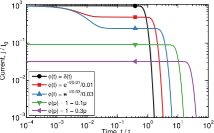
To study the impact of the waiting time distribution on the solution, we initially considered several simple ϕ( )t functions. Time of flight transients were calculated using equation (21), numerically inverting the Laplace transform. Dimensionless results are shown infigure2, where time is scaled to the transit timet_tr = L v/ _d through a sample of thicknessL, and concentration is scaled to the initial concentrationN(0). In this system of units, the normalized drift velocity is equal to 1. We set the normalized diffusion coefficient to D t_{L tr} /d2 = 0.02.

The simplest choice for the waiting time distribution is the Dirac delta,ϕ( )t = δ( )t . In this case, de-trapping occurs instantaneously and consequently has no impact. The system reduces to the standard advection–diffusion equation.

hence decreased effective drift velocity) for increasedτ because of the additional time spent in traps. For the same reason, the current density j falls with increased τ. Nevertheless, the transport is not dispersive, and there exists a clear time-of-flight arrival time.

Afinal option explored is afirst-order truncation of the series expansion of the exponential waiting time distribution in Laplace space:ϕ^( )p ∼ 1− τp, where againτis thefirst moment of the waiting time distribution function. As can be seen from figure 2, the first moment of ϕ controls the long-time behaviour. Higher moments can only influence the behaviour at shorter times, as is demonstrated by the differences between the cases with an exponential distribution and those with the Laplace domain series expansion.

5.2. Relating the waiting time distribution to a density of trapped states

Rather than assuming an ad hoc waiting time distribution, it may be useful to calculate it from a more fundamental physical model. In what follows, we give a specific example for how this might be achieved. We consider a semiconductor with traps that form a density of localized states below the band gap. The release timesϕ( )t are determined by the distribution of these traps in energy space.

To describe this semiconductor, we use a multiple trapping model with a uniform capture (trapping) cross-section [24] for charge carriers. We define the density of localized states to be

g(E), whereE < 0is the energy relative to the conduction band. If the rate of escape from a trap at energy Eis proportional to exp

(

E k T/ _B

)

then

∫

ϕ = ν −ν

−∞

{

}

t g E e t e E

( ) ₀ ( ) E k T exp E k T d , (22)

0

0

[image:8.595.144.360.122.256.2]

B B

whereν₀ is a frequency characterizing the rate of escape from traps. The density of states g(E) can be measured experimentally [25, 26]. In this case we assume an exponential distribution, which occurs in organic and inorganic materials [27,28]. Theng E( ) = eE k T/B c/k T_{B c, whereT}

cis a characteristic temperature that describes the width of the density of states. Equation (22) yields

ϕ( )t = αν₀(tν₀)− −α 1γ α

(

+ 1, tν₀

)

, (23)

whereγ( , )· · is the lower incomplete Gamma function2, andα = T T/ _c. This distribution appears in the literature of the multiple trapping model, for example, equation (9) of [29]. This distribution is normalized, and it has a divergentfirst moment, sufficient to describe dispersive transport [15, 30, 31].

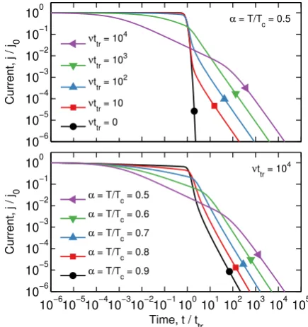
Figure 3 shows typical time of flight transients based on equation (19) together with the waiting time distribution equation (23). Initially, all carriers are assumed to be untrapped. At short times the profiles are classical, with a transition to dispersive behaviour at longer times as the carriers begin to enter the trap states. In the dispersive regime, the sum of slopes is −2, exactly as expected for an exponential density of states [4]. We note that a different form of dispersive transport may arise from a different density of states, and that our model can be readily adapted by evaluating equation (22) with the appropriateg(E) function.

The parameters used forfigure3were chosen as follows. The attempt to escape frequency

[image:9.595.121.523.110.365.2] [image:9.595.140.358.121.353.2]

ν₀ is extremely fast (e.g. ∼1012 Hz [24]), so we consider only the situation where ν₀t_tr ≫ 1.

Figure 3. Modelled current transients for ideal time of flight experiments using the waiting time distribution (23), which was calculated for a semiconductor with an exponential distribution of localized states. An initial trap-free regime transitions into strongly-trap limited dispersive transport. Transport parameters are the same asfigure2, except for the alternative waiting time distribution. These plots were calculated for

ν0ttr= 5×10

5_{. The transition between ‘classical’ and dispersive regimes occurs at}

ν

∼ −

t t/_tr ( t_tr) 1_.

2

The lower incomplete gamma function isγ( , )a z ≡ ∫zta−e−tdt

0 1

We selectedν₀t_tr = 5 × 105forfigure3. The trapping frequencyν,which is a new feature of our model, must be large enough thatνt_tr > 1, otherwise there will be negligible trapping events before the time of flight experiment has concluded. In figure 3(top), we demonstrate the influence of this parameter. It controls the time scale for the transition between classical and dispersive transport. Finally, if the transport is dispersive, the temperatureTmust be below the critical temperatureT_c[24]. We examine the range0.5 ⩽ T T/ _c ⩽ 0.9infigure3(bottom). It can be seen that the slope of the current transient is controlled by the temperature.

Our generalized diffusion equation (18) provides a framework for a unified analysis of transport, whether dispersive or classical. It is pertinent at this point to highlight that in the long time limit, one can make direct connection to the fractional diffusion equation literature [15, 30, 31]. If we consider the Laplace transform of the waiting time distribution (23)

⎛ ⎝

⎜ ⎞

⎠

⎟ ⎛

⎝

⎜ ⎞

⎠ ⎟ 

ϕ απ

απ ν α α ν

= − + − − −

α

p p F p

( )

sin ₀ 2 1 1, ; 1 ; ₀ , (24)

where _{2 1}F is a hypergeometric function, then the small p (long time) representation of this is 

ϕ ( )p ≈ 1 − r p_α α. (25)

Here the coefficients of the pα term have been collected into a single parameter

ν απ απ

≡

α α −

r ₀ /sin , which weights the relative importance of trapping effects. By substituting equation (25) into (18), and taking the limit of small p, one obtains a fractional diffusion equation, with a Riemann–Liouville or Caputo form of the fractional derivative depending upon whether one solves for untrapped charge or total charge. These fractional equations result from a waiting time distribution that was calculated using an exponential density of trap states. It remains to be seen whether alternative ‘fractional’ equations could be formed by considering different distributions for the density of trapped states.

6. Concluding remarks

In this paper we have developed a generalized diffusion equation (18) for transport in disordered materials. This equation is grounded in a phase-space kinetic model that accounts for both free particle transport and trapping/detrapping from localized states, described by a waiting time function ϕ( )t . This model provides a unified framework for the analysis of transport, whether dispersive or not. The nature of the transport is strongly influenced by the waiting time distribution, and in particular, the first moment of this distribution plays a dominant role. By way of example, this model was applied to a disordered semiconductor, obtaining dispersive transport if the density of states is exponential. Other distributions (e.g. a Gaussian) might be expected to yield different detailed behaviour, which could be calculated using the generalized diffusion equation presented here.

Acknowledgments

References

[1] Sokolov I M, Klafter J and Blumen A 2002 Fractional KineticsPhys. Today5548

[2] Robson E R 2006 Introductory Transport Theory for Charge Particles in Gases (Singapore: World Scientific)

[3] Metzler R and Klafter J 2000 The random walkʼs guide to anomalous diffusion: a fractional dynamics approach Phys. Rep.3391–77

[4] Scher H and Montroll E 1975 Anomalous transit-time dispersion in amorphous solids Phys. Rev. B 12

2455–77

[5] Sibatov R T and Uchaikin V V 2007 Fractional differential kinetics of charge transport in unordered semiconductorsSemiconductors41335–40

[6] Saxton M J 2001 Anomalous subdiffusion influorescence photobleaching recovery: a Monte Carlo study

Biophys. J.812226–40

[7] Sagi Y, Brook M, Almog I and Davidson N 2012 Observation of anomalous diffusion and fractional self-similarity in one dimensionPhys. Rev. Lett.108 093002

[8] Kessler D A and Barkai E 2012 Theory of fractional Lévy kinetics for cold atoms diffusing in optical lattices

Phys. Rev. Lett.108 230602

[9] Hilfer R (ed) 2000Applications of Fractional Calculus in Physics Applications of Fractional Calculus in Physics(Singapore: World Scientific)

[10] Barkai E 2001 Fractional Fokker–Planck equation, solution, and applicationPhys. Rev.E63046118

[11] Metzler R, Barkai E and Klafter J 1999 Anomalous diffusion and relaxation close to thermal equilibrium: a fractional Fokker–Planck equation approachPhys. Rev. Lett.823563–7

[12] Jiang H, Liu F, Turner I and Burrage K 2012 Analytical solutions for the multi-term time-space Caputo–Riesz fractional advection–diffusion equations on afinite domainJ. Math. Anal. Appl.389 1117–27

[13] Henry B I, Langlands T A M and Straka P 2010 Fractional Fokker–Planck equations for subdiffusion with space- and time-dependent forcesPhys. Rev. Lett.105 170602

[14] Robson R and Blumen A 2005 Analytically solvable model in fractional kinetic theoryPhys. Rev. E 71

061104

[15] Metzler R and Klafter J 2004 The restaurant at the end of the random walk: recent developments in the description of anomalous transport by fractional dynamicsJ. Phys. A: Math. Gen.37161–208

[16] Bisquert J 2003 Fractional diffusion in the multiple-trapping regime and revision of the equivalence with the continuous-time random walkPhys. Rev. Lett.911–4

[17] Tomovski Ž, Sandev T, Metzler R and Dubbeldam J 2012 Generalized space-time fractional diffusion equation with composite fractional time derivativePhysica A: Statistical Mechanics and its Applications

391 2527–42

[18] Fedotov S and Falconer S 2012 Subdiffusive master equation with space-dependent anomalous exponent and structural instability Phys. Rev.E85031132

[19] Chapman S and Cowling T G 1970Mathematical Theory of Non-uniform Gases: An Account of the Kinetic Theory of Viscosity, Thermal Conduction and Diffusion in Gases (Cambridge: Cambridge University Press)

[20] Bhatnagar P L, Gross E P and Krook M 1954 A model for collision processes in gases. I. Small amplitude processes in charged and neutral one-component systems Phys. Rev.94511–6

[21] Robson R E 1975 Nonlinear diffusion of ions in a gasAust. J. Phys.28523–31

[22] Fried B D and Conte S D 1961The Plasma Dispersion Function (New York: Academic)

[23] Philippa B W, White R D and Robson R E 2011 Analytic solution of the fractional advection–diffusion equation for the time-of-flight experiment in afinite geometryPhys. Rev. E84041138

[24] Tiedje T and Rose A 1980 A physical interpretation of dispersive transport in disordered semiconductors

[25] Tajima H, Suzuki T and Kimata M 2012 Direct determination of trap density function based on the photoinduced charge carrier extraction techniqueOrg. Electron.132272–80

[26] Hulea I, Brom H, Houtepen A, Vanmaekelbergh D, Kelly J and Meulenkamp E 2004 Wide energy-window view on the density of states and hole mobility in poly(p-phenylene vinylene)Phys. Rev. Lett.93166601

[27] Nicolai H T, Mandoc M M and Blom P W M 2011 Electron traps in semiconducting polymers: exponential versus Gaussian trap distributionPhys. Rev. B831–5

[28] Deibel C and Dyakonov V 2010 Polymer-fullerene bulk heterojunction solar cells Rep. Prog. Phys. 73

096401

[29] Jakobs A and Kehr K W 1993 Theory and simulation of multiple-trapping transport through afinite slab

Phys. Rev. B488780–9

[30] Hilfer R and Anton L 1995 Fractional master equations and fractal time random walksPhys. Rev. E 51

848–51