The Primordial Origin and Dynamical Sculpting of Close-In Planetary System Architectures

(1)

The primordial origin and dynamical sculpting of

close-in planetary system architectures

Thesis by

Christopher Spalding

In Partial Fulfillment of the Requirements for the degree of

Doctor of Philosophy in Planetary Science

CALIFORNIA INSTITUTE OF TECHNOLOGY Pasadena, California

2018

(2)

(3)

“Adapt what is useful, reject what is useless, and add

what is specifically your own.”

(4)

ACKNOWLEDGEMENTS

Throughout my academic career, I have been incredibly fortunate to have received the support, love, guidance, mentorship and much else aside from the remarkable people around me. I will begin by thanking my advisor, friend and lead singer of our rock band, Konstantin Baty-gin. I cannot adequately formulate my gratitude for his mentorship into words. He was a postdoc at Harvard when I first requested to begin graduate work with him. It would have been very easy for him to ask me to wait a year – I am very thankful that he did not. Kon-stantin has taught me too many things to list. He taught me celestial mechanics, how to write a paper, inspired me to write my own songs and increased my self-confidence by orders of magnitude. Concisely put, he has been instrumental in letting me become the person I wanted to be. Thank you for everything, and I look forward to a long and enjoyable friendship.

(5)

I would like to thank the other members of my thesis advisory com-mittee, Dave Stevenson, Heather Knutson and Mike Brown. You have each played a key role in guiding my path through grad school. In addition to the faculty on my committee I have had the privilege of interacting with many inspiring individuals at Caltech, be it through course work or simply chance encounters. Particularly in my first couple of years, Andy Thompson and Jess Adkins showed me a spec-tacular sea of knowledge regarding Earth’s oceans. I have had many inspiring conversations with each of you. Andy Ingersoll showed me the wonders of how atmospheres work, including how pressure scales with altitude during a couple of enjoyable nearby hikes we shared. Science is done best when it is collaborative. I have had the privilege of collaborating with many incredible people during my work. Seth Finnegan at Berkeley helped keep my mathematical hammer aimed at the nail stuck in reality. Fred Adams from Michigan is a walking, talking physics textbook that keeps self-writing new pages. Charlie Doering and Glenn Flierl helped me break into the field of population ecology, one that has interested me for years.

Special thanks also go to Mitch Aiken, who showed me the many avenues of outreach available at Caltech. Along a similar vein, I am thankful to the volunteer co-ordinators at the Natural History Museum in Los Angeles, especially Elizabeth Andres, for letting me come and tell people about dinosaurs for a few hours every week.

(6)

photography skills, there would be no evidence I did anything except work during grad school.

The list of friends who have helped support me is a long one: Henry Ngo, Patrick Fischer, Ian Wong, Nancy Thomas, Elizabeth Bailey, Peter Buhler, Peter Gao (extra credit for finding my jokes funnier than even I do), Elle Chimiak and Joe O’Rourke. Each of you have augmented my life in your own particular way.

(7)

ABSTRACT

For centuries, planet formation theories were tuned to reproduce the remarkable coplanarity of our solar system. Specifically, the eight planetary orbital planes exhibit mutual inclinations limited to∼ 1−2 degrees. Furthermore, the misalignment between the Sun’s spin axis and the orbital planes of the planets – the ‘spin-orbit misalignment’– is only about 6 degrees. However, observational characterization of close-in extrasolar planetary systems has revealed an abundance of spin-orbit misalignments ranging all the way from 0 to 180 degrees (Winn et al. 2010). Particularly among the hot Jupiters (giant planets with orbital periods shorter than∼ 1 week), spin-orbit misalignments are more prevalent in systems hosted by stars with effective tempera-tures exceeding about 6200 K. Previous work has suggested that these misalignments arose from violent dynamical interactions that excited planets onto inclined and eccentric orbits, with subsequent tidal circu-larization generating the observed population (Albrecht et al. 2012). This hypothesis has had great difficulty explaining misaligned multi-planet systems, and misaligned orbits of multi-planets that are too distant from their host stars for tidal circularization to act over a sufficiently short timescale. A new mechanism is required.

(8)

impulsively excites large stellar obliquities, ranging between 0 and 180 degrees, in accordance with the observations. In addition, I computed the magnetic torques between the star and disk, finding that a dipole field strength of∼1 kGauss is sufficiently strong to realign the star and disk within typical disk lifetimes (∼ 3 million years). Magnetic fields of this magnitude are observed to persist throughout the disk-hosting stage only for stars less massive than ∼1.2 solar masses (Gregory et al. 2012), corresponding to a main sequence effective temperature of 6200 K, i.e., coincident with the observed break between aligned and misaligned hot Jupiters. Cumulatively, the disk-torquing framework exhibits qualitative consistency with the observed dependence of spin-orbit misalignments upon stellar mass, leaving the theory ripe for a statistical comparison to observations within future work.

(9)

to the orbits of a multi-planet system, its quadrupole moment can disrupt the coplanarity of the system. Indeed, the stellar perturbations are often sufficient to completely destabilize the system (Chapter VI). In addition to constituting an entirely new mechanism of planetary instability, the origin of the required spin-orbit misalignment relates directly back to the discussion above – spin-orbit misalignments may drive the seemingly unrelated Kepler dichotomy.

Finally, I tied in the observation that hot Jupiters appear lonely by demonstrating that stellar contraction can give rise to a secular reso-nance that tilts exterior companions of hot Jupiters, taking them out of transit. Crucially, this resonance is encountered at an earlier time in systems hosting warm Jupiters, precisely owing to their slightly increased orbital distance. I found that the demarcation between a system undergoing secular tilting, and one where the disk quenches the tilting, coincides well with the relatively arbitrary dividing line between hot and warm Jupiters, usually set at orbital periods of about a week.

In summary, I showed that spin-orbit misalignments and orbit-orbit misalignments, measured across a range of planetary size classes, can arise primordially owing to interactions with the host star and binary companions. The importance of the central star had most likely been missed in the previous literature owing to our solar system’s peculiarly wide inner edge at∼ 0.4 AU, as opposed to the more typical

∼ ₀._{1 AU within a galactic setting.} _{In reality, through the wider}

(10)

PUBLISHED CONTENT AND CONTRIBUTIONS

Spalding, C. and Batygin, K., (2014). “Early excitation of spin-orbit misalignments in close-in planetary systems”. In: The Astrophys-ical Journal_{790.1, p. 42. DOI: 10.1088/0004-637X/790/1/42.} C. S. contributed in a conceptual evaluation of the project’s goals, performed calculations and numerical simulations to generate the results, and participated in writing the manuscript. This work was adapted to constitute Chapter II.

Spalding, C., Batygin, K. and Adams, F., C. (2014). “Alignment of protostars and circumstellar disks during the embedded phase”. In: The Astrophysical Journal Letters. 797.2, p. L29. DOI: 10.1088/2041-8205/797/2/L29.

C. S. contributed to the conception of the project, performed calculations and numerical simulations to generate results, and led the writing of the manuscript. This work was adapted to constitute Chapter III.

Spalding, C. and Batygin, K., (2015). “Magnetic origins of the stel-lar mass-obliquity correlation in planetary systems”. In: The Astrophysical Journal_{, 811.2, p.} _82. _DOI: 10.1088/0004-637X/811/2/82.

C. S. contributed to the conception of the project, performed calculations and numerical simulations to generate results, and led the writing of the manuscript. This work was adapted to constitute Chapter IV.

Spalding, C. and Batygin, K. (2016). “Spin-orbit misalignment as a driver of theKepler dichotomy”. In: The Astrophysical Journal. 830.1, p. 5. DOI: 10.3847/0004-637X/830/1/5

(11)

simulations to generate results, and led the writing of the manuscript. This work was adapted to constitute Chapter V.

Spalding, C., Marx, N., W. and Batygin, K. (2018) “The resilience of Kepler systems to stellar obliquity”, The Astronomical Journal, in press. _{preprint found at arXiv: 1803.01182}

C. S. conceived of the project’s primary objectives, performed simulations and calculations, and wrote the manuscript, in ad-dition to mentoring high school student N. W. M in setting up and running some of the simulations. This work was adapted to constitute Chapter VI.

Spalding, C. & Batygin, K. “A Secular Resonant Origin for the Lone-liness of Hot Jupiters”. In: The Astronomical Journal, 154.3, p. 93. DOI: 10.3847/1538-3881/aa8174.

C. S. conceived of the project’s primary objectives, carried out the computations and simulations, and wrote the manuscript. This work was adapted to constitute Chapter VII.

Each of the above publications is reproduced under theAASCopyright Policy (see: http://journals.aas.org/authors/apc.html,

(12)

LIST OF ILLUSTRATIONS

Number Page

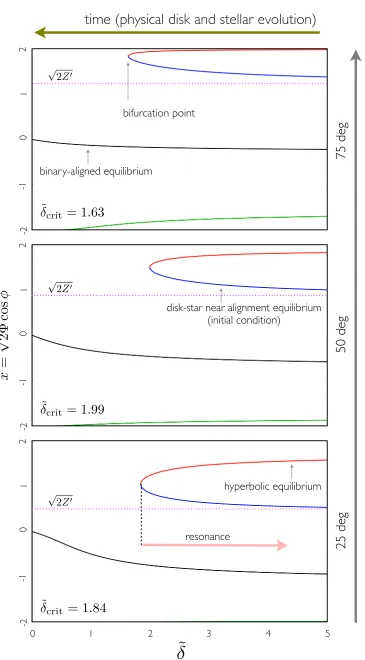
2.1 Equilibria of the Hamiltonian (4.10) as a function of the

resonance proximity parameter ˜δ. The three panels cor-respond to different choices of disk-binary inclination,

namely β0 = 25 deg, β0 = 50 deg, and β0 = 75 deg. The equilibria depicted in black, blue, and green lines are

stable, while that shown as a red line is unstable. As

˜

δ → δ˜_crit_{, two of the four solution merge onto a single} unstable equilibrium. On the contrary, as ˜δ → ∞, a sta-ble equilibrium point approaches perfect alignment with

the disk (shown as a dashed line). . . 30

2.2 Phase-space portraits of the Hamiltonian (4.10) at

differ-ent values of the resonance proximity parameter ˜δ and disk-binary inclination. The colors represent the value

of the Hamiltonian at each contour. In all panels, the

equilibria of the Hamiltonian are shown as gray dots.

The instantaneous disk aligned state is depicted with a

small × symbol. Note that for ˜δ well above ˜δcrit, there exist an equilibrium point in close proximity (but not

exactly corresponding to) the disk aligned state. The

separatrix is shown as a black curve for ˜δ > δ˜crit. On panels corresponding to ˜δ = 0, a white circular orbit that occupies the same phase-space area as the separatrix at

˜

(15)

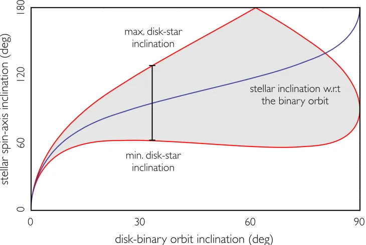
2.3 Resonant excitation of spin-orbit misalignment.

Post-resonant encounter stellar inclination of the star

(mea-sured in a frame coplanar with the binary orbit) as a

function of disk-binary inclination is shown as a purple

curve. Corresponding maximal and minimal spin-orbit

misalignments between the stellar and the disk’s

angu-lar momentum vectors, attained over a precession cycle

are depicted as red curves. Note that the entire possible

range of spin-orbit misalignments is attainable with a

disk-binary inclination β0 6 65 deg. . . 34

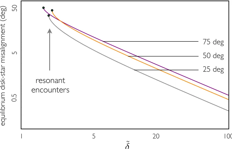
2.4 Gravitationally enforced misalignment between an

equi-librium point (i.e., initial condition) of the Hamiltonian

(4.10) and the disk-aligned state as a function of the

resonance proximity parameter ˜δfor various disk-binary inclinations. The fact that the gravitational equilibrium

does not lie directly on a disk-aligned state provides a

seed inclination for magnetic torques to operate. . . 38

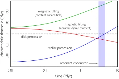
2.5 Characteristic timescales as functions of disk age.

Tak-ing into account the physical evolution of the star and

the disk, the stellar precession timescale is shown as a

blue line, while magnetic tilting timescales assuming a

constant surface field and a constant dipole moment are

shown as green and red curves respectively. The disk

precession timescale is nominally chosen to be 1 Myr, as

in the numerical simulations discussed in the text. The

time interval at which the resonant encounter will take

(16)

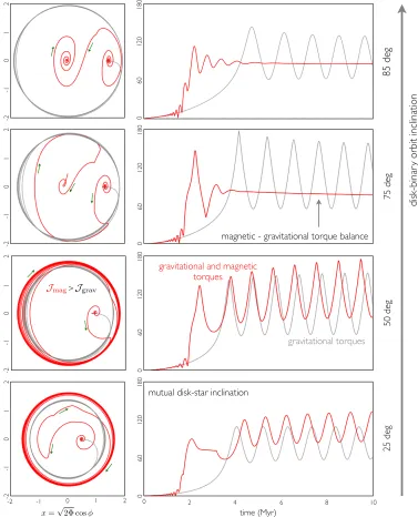
2.6 The results of numerical integration of equations of

mo-tion. The right panels show mutual disk-star

inclina-tion as funcinclina-tions of time, while the left panels show the

phase-space trajectories of the stellar spin axis. The red

curves denote solutions that account for gravitational and

magnetic torques, assuming a constant dipole moment.

Meanwhile, the gray curves show solutions where only

gravitational torques have been retained. While the

lat-ter adhere to the analytic solutions obtained within the

framework of adiabatic theory, the former show

qualita-tive deviations from purely conservaqualita-tive behavior. . . . 42

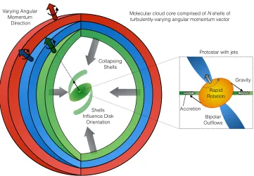
3.1 A schematic of the process described in the text.

Differ-ent shells possess differDiffer-ent angular momDiffer-entum vectors.

In turn, the disk changes its orientation with time.

Grav-itational and accretional torques act between the star and

disk, with bipolar outflows originating from the stellar

spin axis. . . 50

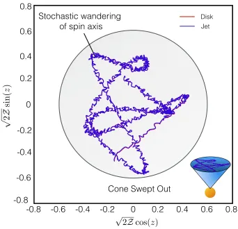
3.2 The paths traced out by the angular momentum vectors

of the disk (red) and star (blue) plotted in canonical

Cartesian co-ordinates (see text). Notice that the red and

blue paths almost exactly overlap. The shaded region

approximately inscribes the cone of gas cleared out by

stellar spin axis-aligned jets. . . 61

3.3 The misalignment between star and disk angular

mo-menta plotted as a function of time. Gravitational

inter-actions alone (blue) are sufficient to suppress significant

misalignment. Accretionary torques (red) further reduce

(17)

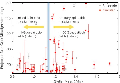
4.1 The observed projected angle between the stellar spin

axis and orbital plane of circular planetary orbits (e ≤ 0.1; red, solid points) and eccentric orbits (e > 0.1; black, faint points) for stars of given masses. There

exists a clear distinction between low-mass stars (M . 1.2M), which display moderate-to small misalignments (especially among circular systems), and the more

mas-sive stars (M & 1.2M), which exhibit misalignments ranging all the way from retrograde-aligned to

prograde-aligned. Measurements of magnetic field strengths

(Gre-gory, Donati, et al., 2012) have revealed that, among

T-Tauri stars, lower-mass stars (similarly, corresponding

to M . 1.2 − 1.4M) possess a much stronger sur-face dipole field than do their higher-mass counterparts.

Specifically, low-mass stars possess fields of ∼1 kGauss in contrast to more modest ∼0.1 kGauss for higher-mass T-Tauri stars. The misalignments data were obtained

fromexoplanets.organd follow the discussion of

(18)

4.2 A schematic to illustrate the origin of each magnetic

torque. The blue region represents the disk material

in-terior to corotation, including the inner wall of the disk,

which super-rotates with respect to the stellar spin,

act-ing both to spin the star up and realign its axis with

the disk’s. The green region is further out and so

ro-tates more slowly, braking the stellar spin and acting to

misalign the star. Red lines represent the requirement

that the entire magnetosphere must be dragged vertically

through the disk once per stellar rotation period if the

star and disk are misaligned. A simple illustration of the

physical mechanism behind each torque is shown on the

right. The colored arrows in the top-left denote the net

torque acting upon the stellar spin axis: green regions

slow down and misalign the star, blue regions speed the

star up and force realignment, whereas red regions act to

brake stellar rotation whilst realigning the stellar

spin-axis. Summed together, the resultant magnetic effect is

(19)

4.3 The approximate magnetic torquing timescale (Talign) as a function of disk-star age for four regimes. The green

lines apply to high-mass stars with a surface field strength

of∼ 0.1 kGauss. Red denotes low-mass stars with a sur-face field strength of∼ 1 kGuass. In both cases, the upper line considers the timescale relevant to a star which is

spinning with a 10 day period whereas the lower line

ap-plies to one with a 3 day period. The stellar spin rate is

assumed to result from the locking to a circumstellar disk

(Koenigl,1991) and so the faster-spinning cases consider

a disk which is truncated at smaller radii, increasing

the magnetic influence. Notice that the dominant

ef-fect upon magnetic torquing timescale is the magnetic

field strength, with timescales proportional to its inverse

square. The timescales increase with time because the

star contracts, leading to an effectively weaker field at

the position of the inner disk. Only for the very

earli-est stages of protoplanetary disk evolution are high-mass

stars’ magnetospheres strong enough to significantly

al-ter their orientation whereas low-mass stars remain

dy-namically influenced by magnetic fields throughout the

(20)

4.4 The time evolution of mutual star-disk inclination. We

consider a binary companion to orbit the system at an

inclination of 30 degrees relative the disk (greater angles

are displayed in Figure 4.5). The companion is

pre-scribed to cause the disk to precess with a 1 Myr period.

The purely gravitational case is shown as a thick, pink

line. The thin, black line denotes evolution in the

pres-ence of the weak fields of high-mass stars (∼0.1 kGauss) and the blue line denotes the evolution corresponding to

the strong fields of low-mass stars (∼1 kGauss). As in previous work (Spalding and Batygin,2014), we find that

a secular spin-orbit resonance is encountered as the disk

loses mass and the star contracts. However, significant

misalignments are inhibited for the stronger magnetic

fields characteristic of low-mass stars whereas the fields

of high-mass stars make no appreciable difference to the

dynamics. Interestingly, the action of magnetic torques

takes the star into alignment with the binary plane, not

the disk plane, suggesting that small misalignments are

indeed a natural outcome of low-mass star evolution,

whereas high-mass stars can take on the full range of

(21)

4.5 Star-disk misalignments as functions of time for a

vari-ety of disk-binary inclinations. This set of figures show

similar information to that shown in Figure 4.4, except

we now illustrate the evolution for a range of angles:

30 deg (top-left), 45 deg (top-right), 60 deg (bottom-left)

and 75 deg (bottom-right). The thick, pink line is the

field-free case, the thin, black line presents the

weak-field (0.1 kGauss) case inherent to high-mass stars and

the blue line denotes the strong-field (1 kGuass) case of

low-mass stars. The over-all pattern is largely similar

up to 60 deg, in that the star is drawn towards a

binary-aligned state over the magnetic realignment timescale.

Not even the strong fields can undo the extreme

reso-nant acquisition of misalignments occurring as a result

of a 75 deg binary inclination. These larger binary

in-clinations are less likely, but raise the possibility that we

may find a rare population of retrograde planetary orbits

(22)

4.6 The time evolution of absolute stellar angular velocity

in the case of a 1 kGauss dipole field, plotted in units

of the equilibrium angular velocity (here corresponding

to an 8 day period). We show the evolution for four

values of disk-binary inclination, increasing from top to

bottom: 30 deg (cyan line), 45 deg (green line), 60 deg

(purple line), 75 deg (orange line). In each case, the

star is prescribed to relax to a disk-locked equilibrium at

an 8 day rotational period over a Kelvin-Helmholtz time.

The relaxation is included in anad hocfashion and so the

exact form of the rotation curves after ∼ 2 Myr is not to be taken too literally. However, as is most apparent for

the higher inclinations, magnetic braking constitutes a

significant mechanism for the removal of stellar angular

momentum. Indeed, for large binary inclinations, the

star can be almost entirely stopped and re-spun within a

(23)

5.1 The amplitude of oscillations in mutual planet-planet

inclinations excited between two initially coplanar,

cir-cular planetary orbits βrel, scaled by twice the stellar obliquity β?. The planets are situated at 0.05 AU and 0.1 AU for 3 different mass configurations: The red line

has a 10 Earth mass planet outside a 1 Earth mass planet,

where blue has the planets switched. The cyan line

aug-ments the inner planet to 100 Earth masses. Notice that

any time the inner planet has more angular momentum,

there exists a peak in the misalignments, representing

resonance. In the limit of large J2, the planets entirely decouple and reach mutual inclinations equal to twice

the stellar obliquity. . . 121

5.2 The maximum number of transits detectable after 22

mil-lion years of integrating Kepler-11 with a tilted, oblate

star. Thex-axis denotes the value ofJ2immediately after disk dispersal (J2,0) and the y-axis represents the stellar inclination. The runs where planets were lost through

in-stability are outlined by a dotted line, which corresponds

closely to the region where only single transits can be

(24)

5.3 Fraction of systems exhibiting each number of transiting

planets from 1 to 7 within the hot (Teff > 6200 K, red bars) and cool (Teff < 6200 K, blue bars) sub-samples of planet-hosting Kepler stars. There were 132 hot stars and

1504 cool stars in the data used, of which 83% and 73%

respectively exhibited single transits. Accordingly,

tran-siting systems around hot stars show a stronger tendency

toward being single, in agreement with the predictions

of our presented model (see text). . . 132

5.4 Probability of the data, given an intrinsic fraction S of

singles out of systems with hot (red line) and cool (blue

line) stars. The separation of the peaks is roughly 2.9σ (as defined in the text). Therefore, to a very high

con-fidence, hot stars possess relatively more singles, as our

hypothesis predicts. . . 134

6.1 A schematic of our numerical simulations. The planetary

system is initialized with coplanar orbits, all sharing a

mutual inclination of β? with the stellar spin axis. The star begins with an oblateness parameter J2 = J2,0which decays exponentially on a 1 million year timescale. The

simulations are carried out using the symplectic N-body

(25)

6.2 The number of planets detectable in transit after 20

mil-lion years of simulation from an initially 2-planet

config-uration. Solid black lines denote the critical obliquity as

a function of J2,0 predicted to reduce the transit number from 2 to 1 according the the formula Spalding and

Baty-gin (2016). The dotted line outlines the region where one

of the two planets was lost owing to dynamical

instabil-ity. We explore the mechanism of instability in more

detail by examining the cases outlined in blue on the plot

for K2-38. . . 147

con-figuration. The dotted line outlines the region where one

or more planets were lost owing to dynamical instability. 151

con-figuration. The dotted line outlines the region where one

or more planets were lost owing to dynamical instability. 152

6.5 The evolution of eccentricity of both planets in the K2-38

system when the stellar obliquity is set at 30◦(blue, inner

planet and red, outer planet) and 20◦ (grey, inner planet

and black, outer planet). For both cases, oblateness

decays from J2,0 = 10

−₂.₆

. The difference in dynamics

between the two cases is profound. Whereas at 20◦ both

planets remain circular, at 30◦both eccentricities begin to

grow in unison at 3.75 Myr. After reaching eccentricities

of roughly 1/2, instability sends the outer planet into the

(26)

6.6 A closer look at the dynamics close to the time of

insta-bility of K2-38 with parmeters β? = 30◦, J2,0 = 10

−₂.₆

.

Top panel: The evolution of eccentricity as a function

of time for the outer planet (blue) and the inner planet

(red). Middle panel: Time evolution of the resonant

ar-gument cos($1−$2)through instability. Notice that the argument librates close to π during the main phase of eccentricity growth (the shaded, blue region), which is

indicative of secular resonant capture. During these

dy-namics,$Û1 ≈ Û$2. Bottom panel: Illustration of ultimate cause of instability. The solid lines illustrate semi-major

axis of the inner (red) and outer (blue) planets, whilst the

dotted lines denote the apocenter (upper) and pericenter

(lower) of the orbits. Secular resonance is broken as the

orbits begin to cross (time≈ 3.98 Myr), and instability

ensues soon after (time≈ 4.36 Myr). . . 167

6.7 Evolution of the orbital inclinations of both planets

com-pared to the locus of $Û1 − Û$2 = 0 as computed from equation 6.18. We plot 4 different cases corresponding

to β? = {30◦, 40◦, 50◦, 60◦} and J2,0 = 10

−₂.₆

. In each

case, blue corresponds to the evolution before instability,

and red after wards (defined as having e1 > 0.01). The solid, dotted and dashed lines denote $Û1 − Û$2 = 0 at times 0.38 Myr (the time of instability for β? = 60◦), 3.75 Myr (instability time for β? = 40◦) and a long-time example of 10 Myr included to illustrate that when

the stellar quadrupole is removed, resonance may still

be encountered if the planetary inclinations are excited

(27)

7.1 A schematic of the set up considered in the text. A

giant planet with mass m2 follows a circular orbit with semi-major axis a1. Exterior, lies a lower-mass planet

m₂ on circular orbit with semi-major axisa2. The exte-rior orbit is forced to undergo nodal regression due to a

combination of stellar quadrupolar potential and secular

perturbations from the inner giant planet’s orbit. The

gi-ant’s orbit, in turn, is regressing mostly owing to secular

perturbations form the stellar oblateness. Initially, the

inner planet regresses faster but as the stellar quadrupole

decays (as a result of physical contraction), a

commen-surability is encountered in the two frequencies, leading

to the secular resonant excitation of mutual inclinations

(28)

7.2 The time evolution of the nodal regression frequencies

for both planets as the host star contracts. The

require-ment to turn a giant planet-super Earth system into an

apparently lonely giant is thatν2 < ν1(i.e., the red line is above the blue line) at the point when the disk dissipates,

such that a point is crossed where the two frequencies

are roughly commensurate. As argued in the text, this

will always happen as the giant grows, but can be

by-passed due to planet-disk interactions. If this is the

picture dominating the hot Jupiter-warm Jupiter

distri-bution, we would expect to see more hot Jupiters with

companions around faster-rotating, massive stars and a

gradual drop in companion fraction toward smaller

semi-major axes. Parameters used in this illustrative figure

are m1/M? = 10

−₃_,

m₂/M? = 10−5, a1 = 0.04 AU, a2 = 0.1 AU, P? = 3 days around a solar mass star. Resonance

(29)

7.3 An illustration of the influence of the disk’s quadrupole.

The solid blue line represents the outer planet’s nodal

regression in the case with no disk, whereas the three

dashed lines represent the case where the disk’s quadrupole

moment is included. When the outer planet is forced to

regress faster than the giant (red line) throughout the

entire disk lifetime, the secular resonant encounter

de-scribed in the text is prevented. The left panel considers

a hot Jupiter, at 0.04 AU interior to a test particle at

0.12 au. The right panel depicts the case for a Warm

Jupiter at 0.1 AU with an exterior test particle at 0.3 au.

The closer, hot Jupiter system encounters the secular

res-onance later (black circle) and so the disk is more likely

to have dispersed, whereas the warm Jupiter system

en-tirely bypasses the secular resonance even for very short

disk lifetimes (e.g., 1 Myr). . . 185

7.4 Loci of systems expected to undergo resonant

excita-tion of inclinaexcita-tion before disk dissipaexcita-tion at 1 Myr (top

panel), 3 Myr (middle panel) and 10 Myr (bottom panel).

Outer companions within the shaded region will not

en-counter the resonance and will remain coplanar with

the inner giant. We have plotted the configuration of

the four systems known where a giant lies interior to a

lower-mass planet. All four lie within the region where

coplanarity is expected to persist around a well-aligned

star. Interestingly, the innermost example, WASP-47,

lies almost exactly on the boundary, consistent with it

being the closest-in known example and only hot Jupiter

(30)

LIST OF TABLES

Number Page

5.1 The parameters of the Kepler-11 system. The mass of

Kepler_{-11g only has upper limits set upon it, but we}

follow Lissauer, Jontof-Hutter, et al. (2013) and choose

a best fit mass of 8 Earth masses here. . . 137

6.1 The parameters of the simulated Kepler systems.

Ini-tially, we set all eccentricities to zero. Date are obtained

from (Jontof-Hutter et al., 2016) and exoplanetarchive. . 144

6.2 The semi major axes and eccentricities of the 4 most

unstable 2-planet systems resulting from our simulations.

For each case where instability occurred, we recorded

the eccentricity and semi-major axis of the remaining

planet, then took the mean of all the results (denoted

by an overbar, with the subscript ‘f’ meaning ‘final,’ ‘i’

representing ‘initial” and the number corresponding to

the particular planet). The mean is only a very general

guideline as to what to expect, but the results suggest

that a population of single-transiting systems that had

undergone our proposed instability mechanism would

be expected to yield an average eccentricity of roughly

(31)

C h a p t e r 1

INTRODUCTION

1.1 From planetary to exo-planetary science

The term “planet” comes from the Greek “to wander,” recapitulating the original realization that the motion of planets across the sky devi-ates from the simple east to west motion of the stars. Even to the naked eye, planets stand apart from stars in that they do not twinkle, Mars has a red hue, and with the aid of a small backyard telescope, the phases of Venus are revealed, in resemblance to those of the moon. Humans have written myths, legends, and creative masterpieces inspired by the planets. But the reality, as is so often the case, goes beyond the imagination of even the most whimsical of tales.

Up until 1995, an extensive literature had been written in the quest to understand the origin of our own solar system. Laplace and Kant had independently come to the correct conclusion that the planets’ birth-place consisted of a disk of gas (Kant,1755; Laplace,1796). This idea was motivated by the coplanar arrangement of the planetary orbits, and has been spectacularly confirmed by relatively recent images from the Hubble Space Telescope.

(32)

(Walsh et al.,2011).

Given the prose above suggesting inward migration, perhaps it should not have been the paradigm-shattering event that it was when the first planet discovered around a Sun-like star, 51 Pegasi b, was a giant planet residing 20 times closer to its host star than the Earth sits in its orbit (Mayor and Queloz, 1995). These planets, known as “hot Jupiters” feature heavily in the following chapters. In order to form such a titan within a disk of gas, a core of solids must first be constructed totalling over 10 Earth masses (Stevenson, 1982; Pollack et al., 1996), such that its gravity attracts a significant amount of gas towards it. This so-called “core accretion” framework was thought impossible within the hot, inner regions of the natal disk. The reason is that water would have evaporated, leaving a lower solid surface density which, together with a reduced cohesiveness between dust particles, would inhibit the growth of larger cores. Consequently, the requisite cores must have formed at distances more similar to Jupiter, before migrating inwards. However, whereas our Jupiter “tacked” and moved back out (because of interactions with Saturn), the hot Jupiters continued their inward march to the inner edge of the disk.

(33)

eccentric-ities bring the closest approach of the planet’s orbit close enough to the host star for tidal deformation to become significant. These tides, raised on the planet, dissipate the orbital energy, reduce the orbital distance, and turn the “cold” Jupiter into a “hot” Jupiter.

As I discuss further below, this second pathway is essentially unique to hot Jupiters, and thus if true would constitute an entirely separate for-mation history for hot Jupiters than for almost all other planets known. Despite this apparent special place for hot Jupiters, the literature has tended toward favouring the high-eccentricity pathway.

1.2 The hot Jupiter debate

For the past 15 years, most of the literature investigating theformation pathway of hot Jupiters has been focused primarily upon deducing theirmigrationpathway. However, since then, numerous other types of close-in planets have come to light. For example, the so-called “warm Jupiters” are giant planets, like hot Jupiters, but instead of possessing week-long orbits, their orbits last between weeks and months. These objects still reside too close-in to have formed via core accretion, but they are too far from the star for tides to have circularized their orbits within a sufficiently short amount of time. In other words, they still must have migrated, but can only have done so owing to interactions with the natal disk.

(34)

found as members of multiple-planet systems – a delicate configuration (see Chapter V) that probably would not have survived the violent events required to excite sufficiently high eccentricities.

With the above discussion highlighting the suspected importance of disk-driven migration for other types of planets, it appears odd that hot Jupiters arrive through an extra formation pathway, one not shared by the warm Jupiters, not shared by the super Earths, and not shared by our own solar system. Before the completion of the work con-tained within this thesis, two pieces of evidence in particular strongly suggested that this special place was appropriate for the hot Jupiters. These were:

1) Hot Jupiters exhibit significant spin-orbit misalignments – mis-alignments between the perpendicular to the orbit and the spin axis of the host star (Winn, Fabrycky, et al.,2010; Albrecht et al.,2012). 2) Hot Jupiters are almost never found to possess close-in companion planets within the same system. (Steffen et al.,2012; Huang, Wu, and Triaud,2016)

Spin-orbit misalignments

With regard to 1), the literature typically assumed that the solar-system’s aligned configuration is overwhelmingly the most likely ini-tial condition for planet formation (Winn and Fabrycky, 2015). In other words, stars and disks were assumed to begin their lives in an aligned configuration. With that picture in mind, the only way to tip stars over with respect to the orbital planes of their planets is through perturbations occurring subsequent to the disk-hosting phase – the high-eccentricity pathway satisfies this requirement well.

(35)

suf-fers in numerous respects upon closer inspection. Specifically, the framework predicts a small but significant population of planets “on the way" towards becoming hot Jupiters. However, fewer such objects are detected than would be predicted form the hypothesis (Dawson, Murray-Clay, and Johnson,2014). Furthermore, under reasonable as-sumptions, the orbital energy deposited within the giant planet during its tidal dissipation is potentially enough to unbind the entire planet (Gu, Lin, and Bodenheimer, 2003). In any case, the process itself is difficult to thoroughly test because it depends upon the abundance of encounters likely to excite sufficient orbital eccentricities. Neverthe-less, estimates typically conclude that under half of hot Jupiters may form this way, though the fraction of misaligned hot Jupiters explained may be larger (Naoz, Farr, and Rasio, 2012).

Given the theoretical difficulty in explaining the properties of hot Jupiters with high-eccentricity migration, in this thesis (Chapters II-VI), I will challenge the above premise that stars and disks form in an initially coplanar configuration. If true, the concerns regarding the high-eccentricity framework are circumvented, as the planetary orbits become misaligned with the central star from the outset. Furthermore, as we shall see, tilting a disk with respect to its central star’s spin axis naturally results from the presence of a gravitationally bound, stel-lar mass companion (Chapter II). Though empirical estimates differ, a fraction of stars close to unity originate in gravitationally-bound multiples (Sadavoy and Stahler, 2017). Accordingly, with the the-ory developed in this thesis, disk-star misalignments aren’t simply possible, they areexpected.

(36)

The previous, leading hypothesis to explain this trend was that mis-alignments occurred around stars of all masses, but that the large convective envelope possessed by the lower-mass stars enhanced tidal dissipation, realigning the star and the planet over time (Winn, Fab-rycky, et al.,2010; Lai,2012; Dawson,2014). Unfortunately, this idea required questionable assumptions to be made regarding the pathway toward tidal dissipation. Specifically, one needs to require that in-clination damps faster than semi-major axis, or any model correcting inclinations would remove the planet from orbit. Furthermore, though more distant planets show a slight trend toward larger misalignments, as expected from a tidal mechanism, the trend occurs too far out to be indisputably tidal in nature (Li and Winn, 2016).

In the thesis, I postulate an alternative idea, one that, like the tilt-ing of the disk itself, plays out durtilt-ing the first few million years of planet formation. Specifically, not tides, but magnetic torques be-tween the young star and its disk realign the lower-mass stars (Chapter IV: Spalding and Batygin 2015). This idea was motivated by ob-servations suggesting a roughly order of magnitude reduced dipole field strength of disk-hosting, high mass stars relative to their lower mass counterparts (Gregory, Donati, et al., 2012). This picture is by no means complete, largely owing to uncertainties stemming from the physics of star-disk magnetic interactions. Nevertheless my work here demonstrates its feasibility, and bypasses the poorly-constrained nature of tidal models.

Orbit-orbit misalignments

(37)

(Steffen et al., 2012; Huang, Wu, and Triaud, 2016). Almost ubiq-uitously, the proposed mechanism is that the dynamically violent na-ture associated with the high-eccentricity migration has removed any close-in planetary companions that may once have existed. Whereas if indeed hot Jupiters form through such a pathway, they would be expected to cast out companion planets, the above concerns regarding high-eccentricity migration suggest an alternative hypothesis may be required.

The alternative model presented in this thesis considers the dynami-cal consequences of forming a close-in companion exterior to a hot Jupiter. In brief, that the gravitational perturbations associated with the contracting, central star initiate resonant dynamics between the two planets. These interactions cause a tilting of the lower-mass planet’s orbit out of the plane of the hot Jupiter (Batygin, Bodenheimer, and Laughlin, 2016; Spalding and Batygin, 2017). Given the preponder-ance of transit data used to infer these patterns, this tilted configuration would be observed as a hot Jupiter without any companion planets. Warm Jupiters escape this resonant tilting because, owing to their larger orbital distances, the stellar oblateness weakens before the disk dissipates. Consequently, the disk anchors the planets within the same plane, despite the resonance, allowing warm Jupiters to coexist with close-in companion planets.

(38)

often leads to dynamical instability, and many of the planets are lost. I have not yet combined these two frameworks. Is an inclined compan-ion to a hot Jupiter dynamically stable over billcompan-ions of years? If not, it would not be detected, meaning that different observational tests are required.

An observational test suggested in this thesis is of a more statistical nature (Chapter VII). In particular, knowing the orbital properties of a giant planet, and its potential exterior companions, we can construct a theoretical parameter-space where the proposed resonant tilting should occur. If exterior planets are frequently found in that region, the model needs to be reconsidered. Only 4 examples exist of close-in giants with exterior companions (Huang, Wu, and Triaud, 2016; Spalding and Batygin,2017). Whereas they are all consistent with my proposed framework, the number is still too small to derive any significant statistical conclusions.

Implications

(39)

The picture conceived by Kant and Laplace was correct in many ways. However, binary stars, the spinning down of planet-hosting stars, and the numerous gravitational perturbations felt within the early stages of the formation of a planetary system all conspire to disrupt coplanarity akin to our solar system in numerous other instances. How might our solar system’s history have been different if the Sun was tilted over? Perhaps it was early on, but the stellar magnetic field righted the system. Potentially, if our system, like most others, possessed close-in super Earth planets the resulting star-planet interactions would have destabilised the solar system.

(40)

C h a p t e r 2

(41)

ABSTRACT

(42)

2.1 Introduction

Nearly two decades after the celebrated radial velocity detection of a planet around 51 Peg (Mayor and Queloz, 1995; Marcy and Butler,

1996), the orbital histories of hot Jupiters, (giant planets that reside within ∼ 0.1 AU of their host stars) remain poorly understood. Con-ventional planet formation theory (Pollack et al., 1996) suggests that in-situ formation of hot Jupiters is unlikely, implying that these objects formed beyond the ice-lines of their natal disks (at orbital radii of or-der∼a few AU) and subsequently migrated to their present locations. The nature of the dominant migration mechanism, however, remains somewhat elusive.

Broadly speaking, the proposed theoretical mechanisms responsible for delivery of hot Jupiters to close-in radii fall into two categories. The smooth migration category essentially argues that large-scale transport of giant planets is associated with viscous evolution of the disk (Lin, Bodenheimer, and Richardson, 1996; Morbidelli and Crida, 2007). More specifically the envisioned scenario suggests that newly-formed giant planets clear out substantial gaps in their protoplanetary disks (Goldreich and Tremaine, 1980; Armitage, 2011) and, having placed themselves at the gap center (where torques from the inner and outer parts of the disk instantaneously cancel), drift inwards along with the gas.

(43)

2012), Kozai resonance with a perturbing binary star (Wu and Mur-ray,2003; Fabrycky and Tremaine,2007; Naoz, Farr, Lithwick, et al.,

2011), and secular chaotic excursions (Lithwick and Wu,2012). From a purely orbital stand point, there appears to be observational ev-idence for both sets of processes. That is, the existence of a substantial number of (near-) resonant giant exoplanets (Wright et al.,2011) and direct observations of gaps in protoplanetary disks (Andrews, Wilner, Espaillat, et al., 2011; Hashimoto et al., 2012) imply that smooth disk-driven migration is an active process. Simultaneously, the exis-tence of highly eccentric planets such as HD80606b (Laughlin,2009) hint at violent migration as a viable option (see however Dawson, Murray-Clay, and Johnson2014).

In the recent years, observations of the Rossiter-McLaughlin effect (Rossiter, 1924; McLaughlin, 1924), which inform the projected an-gle between the stellar spin axis and the planetary orbit (Fabrycky and Winn,2009), have placed additional constraints on the hot Jupiter delivery process. Particularly, the data shows that spin-orbit mis-alignments are generally common within the hot Jupiter population, and the individual angles effectively occupy the entire possible range. Interpreted as relics of hot Jupiter dynamical histories (see however Rogers, Lin, and Lau2012for an alternative view), these observations seemed to strongly favor the category of violent migration mecha-nisms over disk-driven migration, as spin-orbit misalignments are a natural outcome of the former.

(44)

end, Bate, Lodato, and Pringle (2010) hypothesized that stochastic external forces that act on newly formed protoplanetary disks may give rise to spin-orbit misalignment, while Lai, Foucart, and Lin (2011) showed that a mismatch between the stellar magnetic axis and the disk orbital angular momentum vector can be further amplified by magnetic torques.

In a separate effort, Batygin (2012) showed that owing to enhanced stellar multiplicity in star-formation environments (Ghez, Neugebauer, and Matthews, 1993; Kraus et al., 2011; Marks and Kroupa, 2012), secular gravitational perturbations arising from binary companions may torque protoplanetary disks out of alignment with their host stars. This study was subsequently extended by Batygin and Adams (2013), who also considered the dissipative effects of accretion and magnetic modulation of stellar rotation as well as the physical evolution of the star and the disk on the excitation of spin-orbit misalignment. Importantly, the latter study demonstrated that the acquisition of stellar obliquity occurs impulsively, via a passage through a secular spin-orbit resonance.

A distinctive prediction made by the disk-torquing model is the exis-tence of coplanar planetary systems, whose orbital angular momen-tum vectors differ from the spin axes of the host stars. This prediction was recently confirmed observationally by Huber et al. (2013) in the Kepler-56 system. Moreover, the statistical analysis of Crida and Batygin (2014) has shown that the expected spin-orbit misalignment distribution of the disk-torquing model is fully consistent with the observed one.

(45)

spin-orbit misalignments, a thorough examination of the physical pro-cess behind the excitation of inclination is warranted. This is the primary aim of the study at hand. Specifically, in this work, we analyze the passage of the star-disk system through a secular spin-orbit resonance, under steady external gravitational perturbations and magnetically-facilitated tiling of the star. The paper is organized as follows. In section 2, we describe the construction of a perturbative model that approximately captures the relevant physics. In section 3, we describe the characteristic behavior exhibited by the model. We conclude and discuss our results in section 4.

2.2 Model

(46)

numerical calculations.

Physical Evolution of the Protoplanetary Disk and the Stellar

In-terior

Typically quoted lifetimes of protoplanetary disks fall in the range

∼ ₁−_{10 Myr and almost certainly depend on various parameters such}

as the host stellar mass (Williams and Cieza,2011). We adopt several approximations for the physical evolution of the star and disk, which are specific to Sun-like stars, which host the best observationally characterized hot Jupiters. While generally difficult to accurately parameterize, the disk mass can be taken to evolve as (Laughlin, Bodenheimer, and Adams,2004):

M_disk = M

0 disk

1+t/τdisk

. _(2.1)

Interpreting the time derivative of Mdisk to represent the accretionary

flow, following Batygin and Adams (2013) we find that the initial disk mass, M_disk0 = 5×10−2M and evaporation timescale τdisk = 5×

10−1Myr provide an acceptable match to the observations (Hartmann,

2008; Herczeg and Hillenbrand,2008; Hillenbrand,2008).

For simplicity, we model the interior structure of the central star with a polytrope of index ξ =3/2 (appropriate for a fully convective object; Chandrasekhar1939). A polytropic body of this index is characterized by a specific moment of inertia I = 0.21 and a Love number (twice the apsidal motion constant) of k2 = 0.14. Because T-Tauri stars derive a

dominant fraction of their luminosity from gravitational contraction, we adopt the following expression for the radiative loss of binding energy (Hansen, Kawaler, and Trimble,2012):

−₄πR2

?σT_eff4 =

3 5−ξ

GM2

?

2R?2

dR?

(47)

Equation (2.2) effectively dictates the process of Kelvin-Helmhotz contraction, and is satisfied by the solution:

R?= (R?0)

"

1+

5−ξ 3

24πσT_eff4

GM?(R_?0)3t

#−1/3

. _(2.3)

A good match to the numerical evolutionary track of Siess, Dufour, and Forestini (2000) for aM?= 1Mstar can be obtained by assuming an initial radius of R?0 ' 4R and an effective temperature of Teff =

4100K.

Magnetic Torques

In order to model the magnetic disk-star interactions, we consider a T Tauri star possessing a pure dipole magnetic field, whose north pole is aligned with the stellar spin axis. In the region of interest (i.e., in the domain of the disk), the field is current-free and can be expressed as a gradient of a scalar potential:

®

B_dip = − ®∇V. _(2.4)

To retain generality, we take the field to be tilted at an angle βi with

respect to the disk plane into a direction specified by an azimuthal angle ˜φi:

V = B?R?

R?

r 2

P1

0(cos(θ˜))cos(βi) −_sin(β_i)

sin(φ˜i)sin(φ˜)

+cos(φ˜i)cos(φ˜)

P1

1(cos(θ˜))

, _(2.5)

where B? is the stellar surface field and P_lm are associated Legendre polynomials.

(48)

n0, equals the spin rate of the stellar magnetic field, ω. At larger and smaller radii, Keplerian shear will give rise to relative fluid velocity with respect to the stellar rotation. Accordingly, as a result of thermal ionization of alkali metals in the disk (Draine, Roberge, and Dalgarno,

1983), the magnetic field will be dragged azimuthally by differential rotation, whilst slipping backwards diffusively (Livio and Pringle,

1992). Following Armitage and Clarke (1996) we parameterize the magnitude of the azimuthally-induced field Bφ as a fraction, γ = Bφ/Bz, of the vertical component of the dipole field Bz.

As shown by Agapitou and Papaloizou (2000) and Uzdensky, Königl, and Litwin (2002), beyond a critical value of γ ' 1, field lines are stretched to a sufficient degree to reconnect and transition from a closed to an open topology. Thus, the condition |γ| . 1 defines a magnetically-connected region within the disk with ˆa0_in < a0 < aˆ0_out. Outside of this region, we assume there to be no appreciable magnetic coupling to the disk.

The radial profile ofγ is determined by the magnetic diffusivity of the disk, which in turn may be represented by the dimensionless parameter (Matt and Pudritz,2004):

ζ ₌ α

Pm

h

a0, (2.6)

(49)

Königl, and Litwin, 2002)

γ ₌ (a

0_/

a0_co)3/2₋₁

ζ . (2.7)

For our adopted value of ζ this so-called magnetically-connected re-gion does not diverge from the corotation radius by more than ∼ 1%. The above discussion highlights a crucial aspect of the magnetic star-disk interaction, which is discussed in detail by Matt and Pudritz (2004) and Matt and Pudritz (2005). If the disk is truncated at

a0

in > aˆ 0

out, then there is no magnetically-connected region within

the disk. The picture is slightly more complicated for the case where

a0

in < aˆ 0

in, as one may speculate that magnetic effects arising from

differential rotation outside a0_co may cancel those associated with dif-ferential rotation insidea0_coto first order. In all of the following work, we circumvent these issues by assuming a disk-locked condition (Shu, Najita, et al.,1994; Mohanty and Shu,2008) wherea0_in = a0_co, but add a cautionary note that this assumption may lead to somewhat overly favorable results.

In order to derive the analytical form of the torques, we take a similar approach to that of Lai, Foucart, and Lin (2011), and assume the disk to be razor thin. The disk current loops are envisioned to follow the magnetic field lines in a force-free fashion (see, e.g., Krasnopolsky, Shang, and Li 2009; Zanni and Ferreira 2013) and connect onto the stellar surface. Accordingly, the induced azimuthal magnetic field arises from a radial current within the disk (Lai,1999).

The magnitude of the radial current is calculated using Amp`ere’s Law (Jackson, 1998) in the form:

∫

C

®

B · d®l = µ₀

∫ ∫

A

®

(50)

where d®l is a vector path length, dS®is a vector area element andC is a loop encompassing the surface A. J®is the (induced) current density within the disk. Because the induced field is entirely toroidal, we can integrate the left hand side along an azimuthal loop around the disk. This yields:

4πa0Bφ =2πµ0a 0

Kr, (2.9)

whereKr =

∫

Jrdz =2Bφ/µ₀ is the inward radial surface current.

Combining this expression with equation (2.7), we obtain:

K_r = 2Bz

µ₀

(a0/a0_co)3/2₋₁

ζ

. _(2.10)

With an expression for the induced current at hand, we immediately arrive at an expression for the associated Lorentz torque, considering the induced current to interact only with the stellar dipole field:

®

τL = (a0 ρ®ˆ) × (Kr ρ®ˆ × ®Bdip). (2.11)

In the above expression, ˆρ is the radial unit vector in the plane of the disk.

At this point, in order to cast the magnetic torques into a usable form, we project τ®L onto each of the Cartesian axes in the disk’s frame and subsequently integrate over the entire magnetically-connected region:

τi0 =

∫ ₂π

0

∫ a_ˆ_out0

a_co0

®

τL · ®xˆi0 ρdρdφ, _(2.12)

where the subscripti0represents the Cartesian axes in the disk’s frame. With the variables and parameters given above, these torques evaluate to:

τx0 =

2πB?2R?6ζ sin(βi) cos(βi)

3µ0(1+ζ)2(a 0 co)3

(51)

τy0 =

2πB?2 R?6 ζ sin(βi) cos(βi)

3µ0(1+ζ)2(a 0 co)3

sin(φ˜i) (2.14)

τz0 =

4πB?2R?6ζ cos2(βi)

3µ0(1+ζ)2(a 0 co)3

. _(2.15)

Note that for βi > π/2, the star and disk spin in opposite directions, renderinga0_comeaningless. In such a regime, there is no magnetically connected region of the form described above. Indeed, it is unclear how the magnetic field would interact with the disk in this case. For the purposes of our model, we incorporate this loss of a magnetically connected region by artifically forcing the torques to equal zero for angles of βi > π/2. Mathematically, this is done by multiplying the

torques by an approximation to a step functionS(βi)given by:

S(β_i) = ₁−

π_/

2+arctan βi−_`π/2 π

, _(2.16)

where ` = 10−4. The importance of such a term becomes apparent once the torques are coupled to gravity and inclinations above 90 degrees are naturally attained.

Angular momentum transport among neighboring annuli of the disk is facilitated by propagation of bending waves (Foucart and Lai,2011) as well as disk self-gravity (Batygin, Morbidelli, and Tsiganis, 2011) and generally occurs on a much shorter timescale than magnetic tilting of the host star. Taking advantage of this, in our analyses we assume that the effective moment of inertia of the disk around all axes is much greater than that of the star, allowing us to ignore any torques from the star on the disk and to consider−τi0 _{as a back-reaction on the star’s}

dynamics.

(52)

As such, we follow the approach of Peale et al. (2014) and define Euler angles within the binary frame related to the nutation, precession and rotation of the rigid body while assuming exclusively principal axis rotation (this is an excellent approximation for a T-Tauri star, spinning at a period of 1-10 days). Specifically, ˜β is the angle between the central star’s spin axis and the binary orbit normal; ˜Ωis the longitude of ascending node of the star in the binary frame where ˜Ω =0 implies collinear disk and stellar lines of nodes; and the third Euler angle ϕ is the angle through which the star rotates as it spins (ϕ only enters the equations as a rate of change: ϕÛ =ω).

The equations for the evolution of ˜β and ˜Ω, adapted from Peale et al. (2014) are:

dβ˜

dt = −

1 ω

cos(β˜)(−Nx¯sin(Ω˜)+ Ny¯cos(Ω˜))

+ Nz_¯sin(β˜))

, _(2.17)

dΩ˜

dt =−

1

ω _sin(β˜)

Nx_¯cos(Ω˜)+Ny¯ sin(Ω˜)

, _(2.18)

whereN¯iare projected torques. Note that by fixing the disk’s longitude

of ascending node at Ω0 = 0, we have implicitly placed ourselves into a frame coprecessing with the disk’s angular momentum vector. The effect of precession shall be included within the gravitational part of the equations and we need not retain it here.

(53)

The projected quantitiesNi¯are directly related to the torques calculated

above, although the components of the torques in the disk frame,−τi0_,

must first be projected onto the Cartesian axes in the binary frame. Such a projection constitutes a simple rotation of co-ordinates because, as discussed below, the disk-binary inclination is a constant of motion. The rotation angle is fixed at some prescribed angle, β0, anti-clockwise about the x-axis. As such, the components, Ni¯are given in terms of τi

by:

Nx_¯ = −τx0/(I M?R?2), (2.19)

Ny_¯ = −(cos(β0)τy0 −τz0sin(β0))/(I M?R?2), (2.20)

Nz_¯ = −(cos(β0)τx0 +τy0sin(β0))/(I M?R?2). (2.21)

The above equations can be used to analyze the dynamics of the central star owing to its magnetic field interacting with its protoplanetary disk. It is noteworthy that we have made no mathematical assumption of small angles, but physically, we have not taken into account the changes in the parameterized geometry of the problem that arise when mutual disk-star inclinations approach βi → π/2.

Gravitational Torques

Binary Star - Disk Interactions

(54)

The Gaussian averaging method (see Ch. 7 of Murray and Dermott

1999) dictates that in the aforementioned regime, the (orbit-averaged) treatment of the gravitational interactions of the disk-companion sys-tem is mathematically equivalent to considering the companion to be a circular ring with line densityλ = M¯/(2πa¯)and the disk as an infinite series of annular wires at every radius between a0_in and a0_out (Murray and Dermott,1999; Morbidelli, Tsiganis, et al., 2012).

It is well known that within the secular framework, the semi-major axes are constants of motion (Morbidelli, 2002). Consequently, the Keplerian contribution to the Hamiltonian can be dropped, rendering the Hamiltonian of this set up, simply the total gravitational potential energy U possessed by the disk in the field of the companion ring:

U = −

∫

disk

∫

ring

G

r dMdiskdMring, (2.22) where r is the separation between two mass elements dMring

(com-panion), and dMdisk (disk). The integral is carried out over all angles

( ¯φ) within the ring and over all radii (a0) and angles (φ0) in the disk. The evaluation ofr(φ0,a0,φ¯)is a purely geometric problem and can be simplified by approximating a0_out/a¯ 1. Under such an approxima-tion, we expandr to second order in equation (2.22) (first order terms are axisymmetric and therefore cancel out).

In order to compute the integral (2.22), we must specify the disk surface density profile, Σ. For definitiveness, in this work we shall follow (Mestel,1963; Batygin,2012) and adopt

Σ = Σ₀

_a0

0

a0

, _(2.23)

whereΣ0is the surface density at semi-major axisa 0

0. We note that the

(55)

With this prescription, equation (2.22) becomes:

U =−

∫ a_out0

a_in0

∫ ₂π

0

∫ ₂π

0

G

r Σ0a

0 0

¯ M

2π d ¯

φdφ0

da0. (2.24)

Noting thata0_in a0_out, we arrive at the expression for the Hamiltonian. Switching to canonically conjugated variables, we introduce the scaled Poincar´e action-angle coordinates:

Z0 = 1−cos(β0) z0 =−Ω0. (2.25)

This definition of the coordinates differs from the standard definition (see Ch. 2 of Murray and Dermott 1999) in that at each disk annulus, the standard definition multiplies Z0 by dΛ = dm0

√

GM?a0, where

dm0 = 2πΣ0a

0 0da

0

is the mass of the annulus. Thus, for the variables (4.4) to remain canonical, we must also scale the Hamiltonian itself in a corresponding manner:

˘

U = U

2π ∫ a0

out

a_in0 Σ0a

0 0

√

GM?a0da0

= 3n

0 out

8 ¯ M

M?

_a0

out

¯ a

3

Z0− Z

0₂

2

. _(2.26)

This expression agrees with the fourth-order Lagrange-Laplace expan-sion of the disturbing function (Murray and Dermott, 1999), where Laplace coefficients are replaced with their leading order hypergeo-metric series approximations (Batygin and Adams,2013).

The crucial result here is that ˘U does not depend on z0, meaning that the disk inclination is exactly preserved in the binary frame:

dZ0

dt = −

∂U˘

∂z0 = 0 (2.27)

(56)

the constancy of disk-star inclination holds even if an eccentric com-panion is considered. In this case, however, the precession rate is enhanced by a factor of(1+3 ¯e/2).

Disk - Central Star Interactions

As already mentioned above, the spin rates of classical T-Tauri stars fall within the characteristic range of 1 −10 days (Herbst, n.d.; Bouvier,

2013). This results in substantial rotational deformation of young stars. To an excellent approximation, the dynamical response of a spheroidal star to the gravitational potential of the disk can be modeled by considering an inertially equivalent orbiting ring of mass

˜

m =

3M?2ω2R?3I4 4Gk2

1/3

, (2.28)

and semi-major axis

˜

a =

"

16ω2k₂2R?6 9I2GM?

#1/3

. (2.29)

Within the context of this picture, the standard perturbation techniques of celestial mechanics can be applied (Murray and Dermott, 1999; Morbidelli, 2002).

(57)

our problem ( ˜a/a0 . O(10−1)), an octupole-order expansion suffices our needs.

Written in terms of scaled canonical Poincar´e action-angle coordinates (4.4), the Hamiltonian that governs the dynamics of the stellar spin-axis1under the gravitational influence of an infinitesimal wire of mass dm0 _reads:

dH = 1

16 r

GM?

a03

dm0

M?

˜ a

a0

3/2

2−6 ˜Z +3 ˜Z2

× ₂−₆Z0+₃Z02

+12 q

˜

Z(₂−Z˜) −

q ˜

Z3₍₂₋ _Z_˜₎

×

q ˜

Z(₂− Z˜) −

q ˜

Z3₍₂₋_Z_˜₎

cos(z˜−z0)

+ 3 ˜Z Z0 Z˜ −2 Z0 −2cos 2(z˜− z0)

. _(2.30)

As above, to obtain an expression for the Hamiltonian that incorporates the effect of the entire disk, we imagine the disk to be composed of a series of such aforementioned wires and integrate:

H =

∫

dH. _(2.31)

Recalling that the mass of each individual wire comprising the disk is

dm0 = ₂πΣ₀a0

0da 0

, we note that the integral (2.31) runs with respect to the disk semi-major axis.

Because of the stiff dependence of equation (2.30) on a0, the integral (2.31) is only sensitive to the disk’s total mass, and not the location of its outer edge, provided that the latter is substantial (i.e., 10s of AU; Anderson, Adams, and Calvet2013). On the contrary, the disk’s mass is predominantly set by the disk’s size, a0_out:

M_disk = ₂π

∫ a0_out

a0

in

a0Σ₀

_a0

0

a0

da0 ' ₂πΣ₀a0

0a 0

out. (2.32)

(58)

In addition to the disk’s physical properties, we must also prescribe its dynamical behavior to complete the specification of the problem. As already mentioned above, because the Hamiltonian (4.5) is indepen-dent of the angles (i.e., is a Birkhoff normal form), the disk inclination with respect to the binary orbital plane (and thereforeZ0) is conserved, while the disk’s nodal precession rate, ν = dz0/dt, is given by

ν ₌ ∂U˘

∂Z0 =

3n0_out 8

¯ M

M?

a_out0

¯ a

3

1− Z0

. (2.33)

Consequently,H represents a non-autonomous one degree of freedom system.

Because the time-dependence inherent to the problem at hand is par-ticularly simple (z0 = νt),H can be made autonomous by employing a canonical transformation arising from the following generating func-tion of the second kind (Goldstein,1950):

G2 = (z˜−νt)Φ, (2.34)

whereφ = (z˜−νt)is the new angle and the new momentum is related to the old one through:

˜

Z = ∂G2

∂z_˜ =Φ. (2.35)

Accordingly, the Hamiltonian itself is transformed as follows (Licht-enberg and Lieberman,1992):

K = H − ∂G2

∂t . (2.36)

(59)

Following the transformations described above, the Hamiltonian takes on the following form:

K = −Φ+ δ˜

12