promoting access to White Rose research papers
Universities of Leeds, Sheffield and York
http://eprints.whiterose.ac.uk/
This is an author produced version of a paper published in Journal of Applied Statistics.
White Rose Research Online URL for this paper:
Published paper
Jacques, R.M., Fieller, N.R.J., Ainscow, E.K. (2012) A Classification Updating Procedure Motivated by High Content Screening Data, Journal of Applied Statistics, 39 (1), pp. 189-198
A Classification Updating Procedure Motivated by High
Content Screening Data
R.M. Jacques
a, N.R.J. Fieller
b, E.K. Ainscow
ca.
School of Health and Related Research, University of Sheffield, Regent
Court, 30 Regent Street, Sheffield, S1 4DA, UK
b. Department of Probability and Statistics, University of Sheffield, Hicks
Building, Sheffield, S3 7RH
This is a preprint of an article whose final and definitive form has been
published in the Journal of Applied Statistics ©
Taylor & Francis, 2011.
This is the author's version of the work. It is posted here by permission of
'Taylor & Francis' for personal use, not for redistribution.
The definitive version was published in the Journal of Applied Statistics
2012; 1, 189-198.
doi:10.1080/02664763.2011.580335
Abstract
The current paradigm for the identification of candidate drugs within the pharmaceutical industry typically involves the use of high throughput screens (HTS). High content screening (HCS) is the term given to the process of using an imaging platform to screen large numbers of compounds for some desirable biological activity. Classification methods have important applications in high content screening experiments where they are used to predict which compounds have the potential to be developed into new drugs. In this paper a new classification method is proposed for batches of compounds where the rule is updated sequentially using information from the classification of previous batches. This methodology accounts for the possibility that the training data are not a representative sample of the test data and that the underlying group distributions may change as new compounds are analysed. This technique is illustrated on an example data set using linear discriminant analysis, k-nearest neighbour and random forest classifiers. Random Forests are shown to be superior to the other classifiers and are further improved by the additional updating algorithm in terms of an increase in the number of true positives as well as decreasing the number of false positives.
Keywords: Classification, Updating Algorithm, High Content Screening
1. Introduction
The work described in this paper is motivated by the need to use high content screens to identify candidate drugs. The current paradigm for the identification of candidate drugs within the pharmaceutical industry typically involves the use of high throughput screens. A high throughput screen with automated fluorescent imaging platform allows a large number of compounds to be tested in a biological assay in order to identify any activity inhibiting or activating a biological process.
High throughput fluorescent imaging platforms have several advantages over conventional screening techniques that rely on in vitro techniques. The most important of these advantages is that the images contain a wealth of information that can be used to define fully the effects of a compound on cells. It is for this reason that fluorescent imaging assays have been termed high content screening [4]. The study analysed here involves the use of a highly automated robotic system that administer compounds to the cellular assays (each consisting of approximately 300 cells) and then takes measurements of various aspects of cell activity by taking a high content image. These images are then analysed and quantified using advanced imaging algorithms to produce a set of variables.
negative) may result in certain compounds with the potential to be developed further being ignored. Our procedure reduces the number of false hits and thus the amount of ‘wasted effort’ in manually checking false hit images and does not reduce the number of identified true hits (i.e. does not increase the number of false negatives).
In order to sample as diverse a chemical space as possible, each high content screen may extend to a million or more individual assays [11]. This, and the fact that only a small number of compounds in a screen (<1%) have the desired biological effect means that a number of interesting statistical challenges arise when analysing data.
Traditional multi-parametric methods of classification (e.g. linear discriminant analysis) make the assumption that the data used to train the classifier are randomly sampled from the same distribution as the points to be classified in the future [8]. However, in the case of high content screening experiments the training data are from compounds used to validate the experiment. These compounds are selected because of their known biological effects (i.e. both compounds that are known to activate and not to activate the biological process of interest). Hence these data points may not be a representative sample of the data to be classified in the future.
tested by applying it to a high content screening using linear discriminant analysis, k-nearest neighbours and random forests. The results of classifying this way will then be compared with that of the single parameter approach, classical versions of the multivariate classifiers.
2. Example Data Set
The data is derived from a high throughput screen to identify antagonists for a G-Protein Coupled Receptor (GPCR). The GPCR class of proteins represent a major class of drug targets. The assay used here is derived from a generic assay for GPCR activation. A cell line was generated that expressed the receptor of interest and fluorescently tagged protein β-arrestin. Upon activation of the receptor, β-arrestin will
associate with the receptor at the cell membrane and then drive the internalisation of the receptor into intracellular vesicles. The appearance of the fluorescent label thus appears as a punctate distribution. In the presence of an antagonist of the receptor, the receptor does not associate with β-arrestin. Under these conditions, β-arrestin is
uniformly distributed throughout the cell’s cytoplasm. The assay uses an automated imaging platform to visualise the fluorescence distribution within the cells in response to the test compounds. Image analysis algorithms are then used to quantify the distribution of fluorescence as to the degree to which the fluorescence appears punctate to identify active compounds within those screened.
fluorescent label intensity and cell health. In combination, the features potentially report the ability of a test compound to specifically inhibit the receptor of interest, versus non-specific effects such as toxicity.
The data collected from this experiment is contained in three batches. The first 12,285 compounds were selected because of their known properties. This pre-screen batch makes up the training data. The remaining two batches of 33,941 and 33,408 compounds (labelled A and B respectively) yield the test data. 15 variables were measured for each compound; each represents a different aspect of cellular activity. The variables are derived by averaging over the measurements of individual cells in the image.
3. Analysis of High Content Screening Experiments
3.1 Single Parameter Approach
deviations away from the median of the corresponding plate. However, a low Fgrain value can also occur when there are false positives so all wells selected as hits have to be manually checked by eye so that these wells can be excluded [5]. Figure 1 shows the process of selecting hits using this approach.
3.2 Multi-Parameter Approach
Recent developments in the analysis of high content screening data have focused on investigating the implementation of multivariate classifiers. Huang and Murphy [9] and Zhou et al. [17] compare classification using K-nearest neighbours, neural networks, support vector machines, Gaussian mixture models and decision trees with HCS data from location proteomics and time-lapse fluorescence microscopy respectively. Svetnik et al. [15] made a comparison of the random forest classifier, proposed by Breiman [3], with other classifiers for predicting the activities of a compound based on a quantitative description of its molecular structure. The random forest was found to have the highest accuracy amongst all of the classifiers compared. For a general review of classifiers and statistical modelling of high content screening data, see [1, 18].
reduced and therefore enabled rapid progression of the most likely candidate drugs [5].
4. Updating Classification Rules
4.1 Changing Distributions
A fundamental assumption of classical classification techniques is that the various distributions do not change over time [7]. However, in many applications (including high content screens) this assumption is unrealistic and may lead to a decline in performance of a classifier over time. The evolution of class populations in high content screens is due to compounds being analysed in batches. Each of these new batches brings with it new compounds that may have different properties to those in the training data and those in previous batches. Therefore changes to the distributions of the classes and hence the posterior distributions of class membership may be required so that classifier performance does not deteriorate [10].
4.2 New Updating Method
Here we outline the new method for updating the classification rules, which we use in the following section to classify data from a high content screening experiment.
The methodology for the new updating algorithm is as follows. The training data is initially classified using the single parameter plus visual checking approach described in Section 3.1 and a multivariate classifier is constructed using these data. This classifier is then used to classify those compounds which were screened as part of the first batch (in our case batch A) into groups of true hits, non-hits and false hits.
The compounds identified as true hits by the classifier are examined visually by the screening expert to verify the predictions. At this stage all true hits that have been misclassified have their classification labels corrected. A new training data set is now created by combining the data from the batch 1 (the original training data) with the visually checked compounds from batch A.
This new updated training data is used to construct a new multivariate classifier for the classification of Batch B. This part of the algorithm accommodates the possibility that the training data is not representative of the test data by correcting the assumptions on underlying distributions made from the training data.
recommended that each of the batches are manually classified again to see if any true hits were misclassified during previous classification.
4.3 Algorithm
Let the pre-screen training data consist of data where N is total number of observations, the x’s are observations of p variables and the y’s are the class labels (true hit, false hit, non-hit). Given B batches of compounds to be classified, let , be a sequence of test sets each consisting of observations of p variables with unknown class labels. Let , be a sequence of updated training sets that are created by the algorithm.
Step 1: Given the training set , construct a classifier , where given input
the class membership y is given by .
Step 2: (k = 1) Classify the batch of test data using the classifier to give class
labels .
Step 3: Identify observations from the batch of test data such that
= True Hit.
Step 4: Check the classifications of the observations that were identified as true
Step 5: Construct a new training set consisting of the data from and those
observations that were visually checked in step 4.
Step 6: Construct a classifier using the new training set
Set k = k+1 and repeat steps 2-6 until k = B, the number of batches.
Step 7: Manually apply the classifier to batches to identify any True Hits
that have previously been misclassified.
5. Application
5.1 Classification
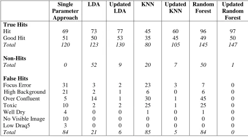
Also note that in Table 1 the true hits group has been broken down into hits and good hits. Good hits are defined as those compounds which show the greatest level of inhibition and are identified by the screening expert. The false hit group has been split into focus error, high background, over confluent, toxic, well dry, no visible image and low draq5. This allows more detailed comparisons to be made.
All of the analysis was conducted in the statistical package R [14]. The random forest classifier was implemented using the randomForest library [12] and the library class [16] was used for the nearest neighbour classifier. When implementing the k-nearest neighbour classifier a leave-one-out cross-validatory approach was used for selecting the value of the parameter k.
true hits than the single parameter approach. The most noticeable improvement in the number of hits selected is found when using the updated random forest, using this methodology identifies 27 more hits than the single parameter approach, and with the number of false positives, the updated random forest only misclassifies one of the hit selected compounds compared to 12, 15, 73, 84, 105 and 134 for the updated k-nearest neighbour, updated linear discriminant analysis, linear discrimiant analysis, single parameter, k-nearest neighbour and random forest respectively. However, the updated random forest failed to identify one good hit that was selected by the single parameter approach.
A detailed comparison of the three non-updating methods used shows that linear discriminant analysis and random forests identify more hits than the single parameter approach but the k-nearest neighbour classifier does not. Linear discriminant analysis also misclassifies fewer compounds as hits but the random forest misclassifies a greater number of compounds with those wells that are toxic and over confluent being the main problem. Additional analysis compared the compounds that were identified as hits and good hits by the four different methods. The aim of this was to see if there were any hits that had been falsely classified as non-hits by the updated random forest, in other words to find if there were any false negatives. The results of this analysis show that there is a minimum of 8 good hits and 29 hits classified as non-hits.
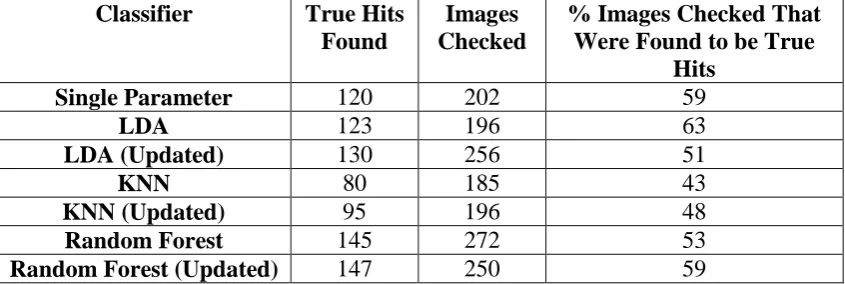
final classifications at Step 7 of the algorithm. Table 2 compares the number of true hits found by each classifier to the number of images that were required to be checked in order to achieve the classification for the two batches of test data. The aim of this analysis was to look at the effort required by the expert to check images with respect to the number of true hits found. The updated random forest identifies the most true hits but also requires the largest number of images to be checked (59% of images checked were found to be true hits). Conversely, linear discriminant analysis has the largest percentage of images checked that turn out to be hits (63%) but it identifies 24 less hits that the updated random forest.
5.2 ROC Analysis
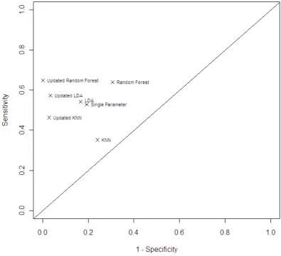
ROC analysis of the classification results was carried out to compare the sensitivity and specificity of the different classifiers. Figure 2(a) is a ROC plot for the classification results shown in Table 1. As the true classifications are not known, sensitivity and specificity have been calculated using only compounds checked visually by the screening expert.
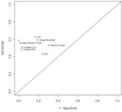
Figure 2(b) is a ROC plot for the results shown in Table 2. Sensitivity has been calculated using the number of images that were required to be check to get the final classifications; i.e.
Specificity was calculated using the usual method (and is the same as for Table 1). Comparing the seven classifiers in this plot shows that updated random forests and updated k-nearest neighbours have higher sensitivity and specificity than the corresponding non-updated classifier but linear discriminant analysis has higher sensitivity than updated linear discriminant analysis. Overall, linear discriminant analysis has the highest sensitivity (63%) with the updated random forest and the single parameter both having the same value (59%). However, the updated random forest identifies 24 more true hits than linear discriminant analysis and 27 more true hits than the single parameter approach.
5.3 Sensitivity of Batch Orderings
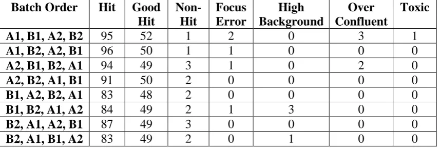
updated random forest as the batch order changed. We divided each of the two batches of test data into two sub-batches (A1, A2, B1 and B2); we then randomly assigned an order to the sub-batches and used the updating methodology to predict the class of the compounds. This process was repeated 8 times so that the predictions made by the model for each sub-batch order could be compared.
Table 3 shows the results of investigating the sensitivity of the classification results when permuting batch orders. It can be seen that there is some variation in the predicted classifications for the different batch orders. The most noticeable difference appears to be between those orderings which start with batch A and those which start with batch B. A detailed comparison of this difference shows that when a sub-batch from batch A is the first to be classified there are more hits from batch A identified than when a sub-batch from batch B is the first to be classified. Although the results of classification vary as the batch order is permuted we suggest that the updating algorithm approximately converges to the same classifications.
6. Discussion
As discussed in section 4.1, population drift may lead to a decline in performance of a classifier over time. We have attempted to combat this problem by continually updating the classifier each time new information is available; however, we suggest that a substantial drift in the populations may cause the model to change sufficiently so that misclassification occurs for the training data and the previously classified test batches. In other words, the model may change so that compounds that were previously classified correctly are now misclassified. It may be possible it identify when this occurs by checking each new model to see how well it predicts the classifications of the original data. In such cases, an alternative approach based on the method of Biernacki et al. [2] may be appropriate.
The results of investigating the sensitivity of batch ordering in Section 5.2 suggest that the model approximately converges to the same classification. However, we suggest that it may be of interest to investigate this further by considering larger numbers of batches. It is possible to optimise the ordering of the batches before they are classified by the algorithm, however, any increase in accuracy would have to be balanced against the time taken to implement it.
When we applied the multivariate classifiers in Section 5 we did not directly consider the incorporation of prior knowledge nor the unequal cost of misclassification. In some cases these could be specified and incorporated into the classifiers at various points in the algorithm. There would be the opportunity to vary the costs at each step in the algorithm but this has not been explored further in the current study.
In conclusion, random forests were shown to be superior to the single parameter approach and the other classical multivariate classifiers. They were further improved by the additional updating algorithm in terms of an increase in the number of true positives and a decrease in the number of false negatives.
7. Acknowledgements
8. References
[1] E.K. Ainscow, Statistical techniques for handling high content screening data, European Pharmaceutical Review 5 (2007).
[2] C. Biernacki, F. Beninel and V. Bretagnolle, A Generalized Discriminant Rule when Training Population and Test Population Differ on their Descriptive Parameters, Biometrics 58 (2002), pp. 387-397.
[3] L. Breiman, Random Forests, Mach. Learn. 25 (2001), pp. 5-32.
[4] P.A. Clemons, Complex phenotypic assays in high-throughput screening, Curr. Opin. Chem. Biol. 8 (2004), pp. 334-338.
[5] E.L. Cooke, E.K. Ainscow, A. Hargreaves, E. Sullivan, P. Alcock, J. Ellston, S. Peters, J. Major, J. Wannop, H. Allen, D. Plant, S. Coundhry, R. Hicks, E. McCall, J. Shaw and L. Ronco, G-Protein-Coupled Receptor High-Throughput Screen Using Norak Transfluor® Technology and the IN Cell Analyser 3000, Proceedings of the SBS 9th Annual Conference 2003.
[7] D.J. Hand, Construction and Assessment of Classification Rules, Wiley, Chichester, 1997.
[8] D.J. Hand, Classifier technology and the illusion of progress, Statist. Sci. 21 (2006), pp. 1-14.
[9] K. Huang and R.F. Murphy, Boosting accuracy of automated classification of fluorescence microscope images for location proteomics, BMC Bioinformatics 5 (2004).
[10] M.G. Kelly, D.J. Hand and N.M. Adams, The impact of changing populations on classifier performance, Proceedings of the fifth ACM SIGKDD International Conference on Knowledge Discovery and Data Mining 1999.
[11] B.A. Kenny, M. Bushfield, D.J. Parry-Smith, S. Fogarty and J.M. Treherne, The application of high-throughput screening to novel lead discovery, Prog. Drug Res. 51 (1998) pp. 245-269.
[12] A. Liaw and M. Wiener, Classification and Regression by randomForest, R News 2 (2002) pp. 18-22.
[14] R Development Core Team, R: A language and environment for statistical computing, R Foundation for Statistical Computing, Vienna, 2009.
[15] C. Svetnik, A. Liaw, C. Tong, J.C. Culberson, R.P. Sheridan and B.P. Feuston, Random Forest: A classification and regression tool for compound classification and QSAR modelling, J. Chem. Inf. Comput. Sci. 43 (2003), pp. 1947-1958.
[16] W.N. Venables and B.D. Ripley, Modern Applied Statistics with S. (Fourth Edition), Springer, New York, 2002.
[17] X. Zhou, X. Chen, K.L. Liu, S. Lyman, R. King and S. Wong, Time-Lapse Cell Cycle Quantitative Data Analysis Using Gaussian Mixture Models, in Life Science Data Mining, World Scientific, Singapore, 2007.
Table 1: Observed classifications of hit selected compounds
Single Parameter
Approach
LDA Updated
LDA
KNN Updated
KNN Random Forest Updated Random Forest True Hits
Hit 69 73 77 45 60 96 97
Good Hit 51 50 53 35 45 49 50
Total 120 123 130 80 105 145 147
Non-Hits
Total 0 52 9 20 7 50 1
False Hits
Focus Error 31 3 2 23 3 7 0
High Background 21 2 1 6 0 6 0
Over Confluent 5 14 1 30 1 45 0
Toxic 10 2 2 25 1 25 0
Well Dry 4 0 0 1 0 1 0
No Visible Image 10 0 0 0 0 0 0
Low Draq5 3 0 0 0 0 0 0
Table 2: Comparing the number of hits found to the number of images checked for different classifiers
Classifier True Hits
Found
Images Checked
% Images Checked That Were Found to be True
Hits
Single Parameter 120 202 59
LDA 123 196 63
LDA (Updated) 130 256 51
KNN 80 185 43
KNN (Updated) 95 196 48
Random Forest 145 272 53
Table 3: Observed classifications of hit selected compounds using updated random forests with different batch orders
Batch Order Hit Good
Hit
Non-Hit
Focus Error
High Background
Over Confluent
Toxic
A1, B1, A2, B2 95 52 1 2 0 3 1
A1, B2, A2, B1 96 50 1 1 0 0 0
A2, B1, B2, A1 94 49 3 1 0 2 0
A2, B2, A1, B1 91 50 2 0 0 0 0
B1, A2, B2, A1 83 48 2 0 0 0 0
B1, B2, A1, A2 84 49 2 1 3 0 0
B2, A1, A2, B1 87 49 3 0 0 0 0