Nonlinearities in the binocular combination of luminance and contrast

White Rose Research Online URL for this paper:

http://eprints.whiterose.ac.uk/75356/

Version: Accepted Version

Article:

Baker, Daniel H orcid.org/0000-0002-0161-443X, Wallis, Stuart A, Georgeson, Mark A et

al. (1 more author) (2012) Nonlinearities in the binocular combination of luminance and

contrast. Vision Research. pp. 1-9.

https://doi.org/10.1016/j.visres.2012.01.008

[email protected] https://eprints.whiterose.ac.uk/ Reuse

Items deposited in White Rose Research Online are protected by copyright, with all rights reserved unless indicated otherwise. They may be downloaded and/or printed for private study, or other acts as permitted by national copyright laws. The publisher or other rights holders may allow further reproduction and re-use of the full text version. This is indicated by the licence information on the White Rose Research Online record for the item.

Takedown

If you consider content in White Rose Research Online to be in breach of UK law, please notify us by

Nonlinearities in the binocular combination

of luminance and contrast

Daniel H. Baker, Stuart A. Wallis, Mark A. Georgeson & Tim S. Meese

School of Life & Health Sciences, Aston University, Birmingham, B4 7ET, UK

email

: [email protected]

Abstract

We studied the rules by which visual responses to luminous targets are combined across the two eyes. Previous work has found very different forms of binocular combination for targets defined by increments and by decrements of luminance, with decrement data implying a severe nonlinearity before binocular combination. We ask whether this difference is due to the luminance of the target, the luminance of the background, or the sign of the luminance excursion. We estimated the pre-binocular nonlinearity (power exponent) by fitting a computational model to ocular equibrightness matches. The severity of the nonlinearity had a monotonic dependence on the signed difference between target and background luminance. For dual targets, in which there was both a luminance increment and a luminance decrement (e.g. contrast), perception was governed largely by the decrement. The asymmetry in the nonlinearities derived from the subjective matching data made a clear prediction for visual performance: there should be more binocular summation for detecting luminance increments than for detecting luminance decrements. This prediction was confirmed by the results of a subsequent experiment. We discuss the relation between these results and luminance nonlinearities such as a logarithmic transform, as well as the involvement of contemporary model architectures of binocular vision.

Keywords:

binocular vision, luminance, contrast, matching, binocular summation

1 Introduction

Binocular combination of luminance has been studied for over 150 years (e.g. Fechner, 1860). A typical experimental paradigm involves matching the brightness (i.e. the perceptual experience of luminance) of a standard binocular stimulusÑwith the same luminance in each eyeÑto a matching stimulus with different luminances in each eye. By varying the interocular ratio of luminances in the matching stimulus, an equibrightness contour can be constructed, on which each point represents a stimulus combination (L, R) with equivalent brightness to the standard (B) (see Levelt, 1965; Engel, 1970; Anstis & Ho, 1998).

Figure 1: Equibrightness contours for stimuli with various luminance levels in each eye. (a) Data are replotted from Engel (1970; Figure 5a) for luminance increments against a dark background, normalized to the standard luminance. Results are averaged over six target sizes and two observers. (b) Data are replotted from Anstis & Ho (1998; Figure 9c). The conditions are similar to those in (a) except they are for luminance decrements against a light background (0.7¡ disc, decrement of 70% of background luminance, data for one observer). In both panels, the thin lines/curves show predictions for linear, quadratic and winner-take-all combination rules, as described in the text. We use the term ÔexcursionÕ to mean Ôdifference from backgroundÕ, which can apply to increments or decrements of luminance, or contrast.

This finding is typical when the target region involves luminance increments against a dark background (Levelt, 1965; Engel, 1970; Anstis & Ho, 1998). However, very different results have been reported when the target luminances are lower than their background (Anstis & Ho, 1998). For this arrangement, the results are much closer to the winner-take-all prediction, implying that the eye viewing the darker target (i.e. the greater luminance excursion relative to the background) determines perceived brightness (see Figure 1b).

What is the critical factor for obtaining these different types of results (Fig. 1)? There are three possibilities: the absolute luminance of the target, the absolute luminance of the background, and the polarity (increment or decrement) of the target relative to the background. To answer this question and to better understand the rules of binocular combination, we performed a series of binocular luminance matching experiments for a stimulus set that included both increments and decrements in luminance and combinations of the two (i.e. changes in contrast). Our results are described by a simple equation and discussed in relation to other results in the literature, similarly (re-)analysed. We also discuss more elaborate models, such as a contemporary binocular gain control model, and consider contrast metrics that might be applied to increment and decrement stimuli.

2 Methods

2.1 Apparatus & Stimuli

All stimuli were presented on a Clinton Monoray monitor using a ViSaGe stimulus generator (Cambridge Research Systems, Kent, UK) controlled by a PC. Ferro-electric shutter goggles (CRS, FE-1) allowed presentation of different stimuli to the left and right eyes with negligible crosstalk. The monitor was gamma corrected using a four-parameter function that accounted for the true luminance output at an input level of 0 (i.e. the Ôblack levelÕ). This ensured that a dark background was as close to 0 luminance as possible. We measured the luminance range using a photometer (Minolta LS-110) as having a

minimum of <0.01cd/m2 and a maximum of

160cd/m2. All luminances were subject to a further eightfold attenuation (0.9 log units) by the frame-interleaving shutter goggles, which are equivalent to a neutral density filter. All luminances reported below are those at the eye, following this attenuation.

stimuli are shown in Figure 2. The luminances of the standard were 1, 2, 4 and 8 cd/m2 for the increment on a dark background. For the mid-grey background, standard luminance excursions for increments and decrements were ±0.5, 1, 2 and 4 cd/m2. For the bipartite field, the standard contrasts were 5, 10, 20 and 40%, where contrast

is percent Michelson contrast (=100*(Lmax

-Lmin)/(Lmax+Lmin), where L is luminance).

(b)

(c)

(d)

(a)

Figure 2: Example stimuli and details of experimental conditions. (a) Luminance increment on a dark background (<0.01cd/m2). (b) Luminance increment on a mid-grey background (10cd/m2). (c) Luminance decrement on a mid-grey background. (d) Bipartite stimulus used in the contrast conditions. In the experiments, the square background had a width of 18.5¡.

2.2 Procedure

Experiments were conducted in a windowless room, in which the only light source was the monitor. Observers viewed the display from a distance of 57cm, with their head in a support on

which the goggles were mounted. The

experiments were carried out in separate sessions for each target and background type. Within each session, blocks of trials were run with trials interleaved to measure the point of subjective equality for an individual ratio of left:right and right:left eye intensities.

A two-interval matching procedure was used to estimate the point of subjective equality at which the standard and matching stimuli appeared equal in luminance or contrast. The standard always had the same luminance or contrast in each eye, the magnitude of which was varied experimentally. The matching stimulus had a fixed ratio of luminance (or contrast) across the eyes, the absolute magnitude of which was controlled by a pair of 1-up, 1-down staircases (Meese, 1995) moving in logarithmic steps of luminance (or

contrast). The ratios of left:right eye magnitude were 0, 0.16, 0.32, 0.51, 0.73 and 1, with equivalent values for the right:left eye ratios. Stimuli were presented for 200ms, with an interstimulus interval of 400ms. The staircase data were fit with a cumulative log-normal function using Probit analysis (Finney, 1971) to estimate the point of subjective equality, which was plotted as a function of left- and right-eye intensity (see Figures 3-6). Note that for data gathered this way, the error bars lie on radial lines that converge at the origin1.

2.3 Observers

Two of the authors served as observers (DHB & SAW). Both were psychophysically experienced and had normal stereopsis, no abnormalities of binocular vision and no need for optical correction.

3 Results

Results for luminance increments on a dark background are shown in Figure 3. These are consistent with typical findings in the literature (Levelt, 1965; Engel, 1970; Anstis & Ho, 1998), showing near-linear behaviour for much of the function but folding back near to each axis. The linear portion of the functions extend over a greater range at higher standard luminances (stated in each panel), particularly for DHB.

For increments on a lighter (mid-grey)

background, the results were markedly different (Figure 4), with fewer points falling near the linear predictions shown by the oblique dotted lines. These results imply a stronger nonlinearity underlying binocular combination on a light background than on a dark background, although the nonlinearity is not as severe as winner-take-all behaviour (dashed lines).

This change in character could be caused by either the higher background luminance or the smaller difference between background and target luminances in this condition. Legge & Rubin (1981) reported similar functions for full-field luminance increments on a background (pedestal) luminance of 10cd/m2.

1cd/m

2cd/m

8cd/m

4cd/m

1cd/m

2cd/m

8cd/m

4cd/m

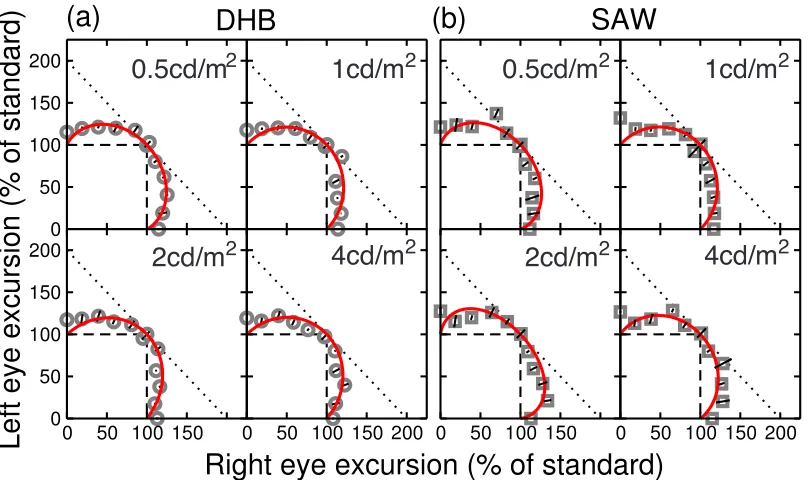
Figure 3: Results for luminance increments against a dark background. Data are normalized to the appropriate standard luminance and shown for two observers in different panels. The standard luminance is given in the upper right corner of each plot and the background luminance was always <0.01cd/m2. The error bars (showing ±1SE) are radial because the matching luminances for the left and right eyes were constrained to be a fixed ratio for each point (see the Procedure section). In most cases these are smaller than the symbols. The dotted and dashed lines show predictions of linear and winner-take-all combination rules respectively (see Figure 1). Curves are the best fit of an equation described in the text, which had one free parameter.

0.5cd/m

1cd/m

4cd/m

2cd/m

0.5cd/m

1cd/m

4cd/m

2cd/m

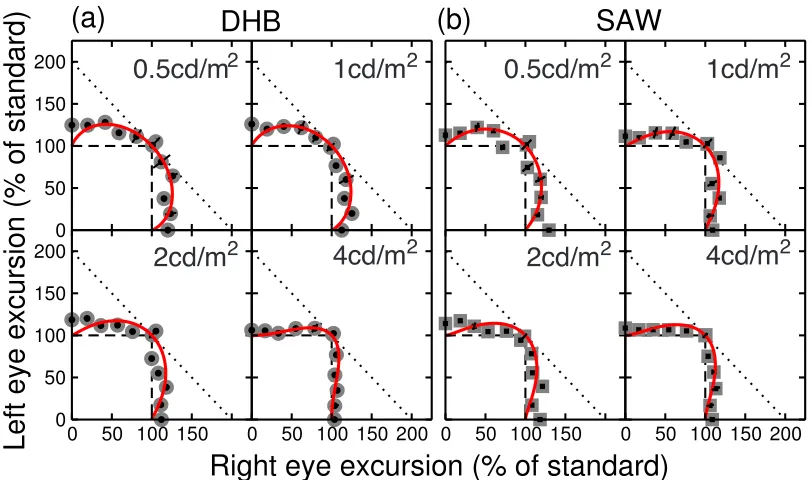
Figure 5 shows results for a condition in which the background luminance (10 cd/m2) was the same as in the previous experiment but the central target luminance was lower than this (i.e. it was a luminance decrement). The red curves fall increasingly close to the winner-take-all predictions as the standard decrement becomes larger. This result is consistent with the findings of Anstis & Ho (1998) and is most profound for the greatest decrements, as we

demonstrate and discuss in the modeling section below.

In a fourth condition, we manipulated target contrast using a bipartite field as the stimulus. The curves measured in this condition (Figure 6) resemble those for decrements on a mid-grey background (Figure 5). We also found similar results for one observer (DHB) using a 1c/deg Gabor patch as a target (not shown).

0.5cd/m

1cd/m

4cd/m

2cd/m

0.5cd/m

1cd/m

4cd/m

2cd/m

Figure 5: Results for luminance decrements on a mid-grey background (10cd/m2), plotted in the same format as Figure 3. Note that here the luminance excursion was a reduction in luminance relative to the background.

4 Computational modeling

4.1 A descriptive model

Several computational models have been proposed to describe binocular luminance and contrast matching results (see Grossberg & Kelly, 1999 for a review). One of the earliest and most general is the equation proposed by the physicist Erwin Schršdinger (1926; see MacLeod (1972) for details). This is defined as,

B

=

L

2"

₊

_R

L

+

R

,

where L and R are the left and right eye absolute luminance deviations (e.g. L = abs(Lcentre-Lsurround))

or, for the bipartite fields, target contrasts, and γ is the only free parameter. Varying γ produces a family of equibrightness contours of differing curvature, as shown in Figure 7a. Note that the

denominator term influences the overall

5%

10%

40%

20%

5%

10%

40%

20%

Figure 6: Results for the bipartite stimulus for which contrast matching was performed against a mid-grey background (10cd/m2). Data are plotted in the same format as Figure 3, except that here the excursions refer to Michelson contrast.

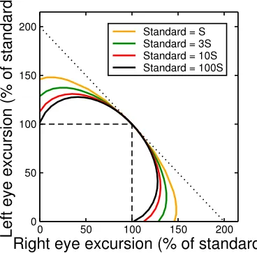
Figure 7: Example luminance- or contrast-matching predictions for equation 1. (a) Equibrightness curves produced by equation 1 for different values of γ. The dotted and dashed lines indicate linear and MAX operations for comparison. (b) Example fit of equation 1 to data for DHB for a standard luminance increment of 4cd/m2 on a dark background. Data are normalized to the standard luminance and the error of the fit was calculated in the radial direction.

Equation 1 provides a good description of the family of curves obtained in binocular luminance and contrast matching experiments. The value of the single parameter (γ) provides a quantitative index of the nonlinearity implied by an equibrightness contour. We exploit this property in order to simplify the presentation of our results and to address the relationship between the effects of target and background luminance in binocular combination.

Each set of equibrightness data was normalized by expressing it as a percentage of the

luminance (or contrast) of the appropriate standard. We then used a simplex algorithm (in Matlab) to find the value of γ that minimised the root mean square (RMS) error between model and data in logarithmic (dB) units and in the radial direction. An example fit is shown in Figure 7b and model curves for each condition are plotted in Figures 3-6. Fits produced a mean

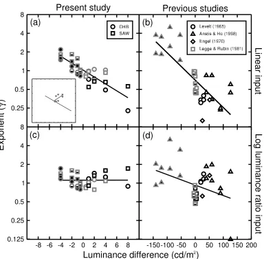
RMS error across the data set of 0.83dB (N=32

Figure 8: Fitted exponents as a function of luminance difference between target and background. (a) Exponents from the present study (the parameter γ in equation 1). (b) Exponents for fits to data from the literature. (c,d) Equivalent to (a,b) but using the log luminance ratio between target and background as the input to equation 1. Symbol conventions follow those of Figures 3-6, with symbol edges denoting background luminance (dark or grey), and symbol centres indicating either increment, decrement or edge-contrast. Symbol shapes indicate observer (a, c) or study (b, d), as detailed in the figure legends, and are unrelated to the shape of the target in a given experiment. Negative luminance differences indicate decrements (where the target is lower in luminance than the background). Values for contrast are also plotted this way, except for in the inset to panel (a) (see text).

As might be expected from examining the raw data, increments tend to produce lower exponent values (i.e. less nonlinear behaviour) than decrements. Figure 8a shows the fitted exponents plotted against the luminance difference between target and background (negative differences indicate decrements). The relationship between luminance difference and exponent is monotonic and approximately linear when plotted with a logarithmic ordinate (as here). Also included are exponent values for the bipartite contrast condition (data from Figure 6). These are plotted against the luminance difference between the background and the decrement portion of the bipartite field. This provides a good correspondence with the exponents from the other conditions, whereas plotting the exponent against the difference

between the background and the increment portion does not (see inset to Figure 8a). This provides a powerful demonstration that the decrement region of the bipartite field

determines the character of binocular

combination (when inputs are expressed in linear units Ð see below).

study. Neither plot (Figure 8a or 8b) appears well disposed to delivering a precise relation between luminance difference and exponent. However, the clear message from both analyses is the general trend that the exponent increases

as the luminance difference decreases.

Luminance increments tend to produce quasi-linear binocular summation (low exponents,

g~0.25-0.5), while luminance decrements

promote winner-take-all (high exponents, g ~2-4).

4.2 Metrics for luminance and contrast

One of the central aims of this study was to attempt to understand binocular matching for luminance increments, luminance decrements

and contrast changes within a single

framework. To do this it is necessary to derive an appropriate metric that can describe all three conditions. Plotting results as luminance and contrast excursions (Figs 3-6) is equivalent to

using the delta contrast metric (D =

∆L/Lbackground; see e.g. Peli, 1997), which is

linear with respect to _∆L for both increments and decrements. We wondered whether a luminance nonlinearity could account for the variation in exponent value that we found when the difference between luminance target and background was varied (Figure 8a).

One commonly used metric is Michelson contrast (M =(Lmax-Lmin)/(Lmax+Lmin)), which is

linear with _∆L for DC-balanced luminance

excursions (e.g. a sinusoidal or bipartite stimulus), and mildly nonlinear for increments and decrements against a light background. However, it is not useful for increments against a dark background, since it produces M=1 for all target luminances (when Lmin = 0, M =

Lmax/Lmax).

An alternative metric for contrast is that proposed by Whittle (1986), which is similar in form (W = (Lmax-Lmin)/Lmin) to the Michelson

contrast equation. This metric produces an

output which is linear with ∆L for all

increments but nonlinear for both decrements

and DC-balanced contrast. Although W was

first proposed to explain luminance

discrimination (i.e. objective performance) data, it is also relevant to matching and scaling (i.e. subjective perceptual) tasks (Whittle, 1992). We found that using W as the input to equation 1 reduced but did not eliminate the dependency of g on luminance difference (not shown).

Our reviewers suggested using a logarithmic transform on the ratio of target and background

luminances. Specifically, |log(Ltarget/Lbackground)|

has the desirable properties of accelerating (with respect to ∆L) for decrements (when Ltarget < Lbackground) and saturating (with respect

to _∆L) for increments (when Lbackground < Ltarget).

(Note that this is equivalent to taking the difference of log luminances). This log luminance metric successfully removed the

dependency of γ on signed luminance

difference for our data (Figure 8c), with the

caveats that Lbackground = 1 for a dark

background to avoid division by zero, and that for contrast stimuli Ltarget was the luminance of

the dark part of the stimulus (see Figure 8a). The slope of the best fit regression line reduced to near zero, and the (geometric) mean exponent value was γ=1.11. Using the log luminance difference did not increase the number of free parameters (this remained at one per curve), and did not affect the goodness of fit (mean RMS error was 0.83dB using both methods).

We confirmed that the log luminance ratio removed the effect of luminance sign on the exponent in equation 1 by calculating the

Pearson correlation between luminance

difference and exponent. For the present data, the correlation was highly significant (R2=0.61, p<<0.01) for linear scaling (Figure 8a), but not significant (R2=0.0002, p=0.94) for the log luminance metric (Figure 8c). For the data from previous studies, the correlation was greatly reduced (from R2 = 0.55 to R2 = 0.13) by the use of the log luminance ratio. Although both correlations were significant at p<0.05, the latter correlation (Figure 8d) was strongly influenced by the outlier sitting on the x-axis of this panel. Removing this outlier further reduced the correlation, below the level of significance (R2 = 0.10, p>0.06). These analyses demonstrate that the log luminance ratio successfully accounted for the apparent change in nonlinearity as a function of luminance difference between target and background.

4.3 Binocular summation

Binocular summation is the improvement in sensitivity for two eyes compared with one. If luminance increments are processed in a more linear fashion than decrements, they should also produce higher binocular summation ratios (BSRs). This is because the amount of binocular summation is controlled by the

nonlinearities placed before binocular

assume that the binocular response can be approximated as resp = Lm + Rm, where L and R are the input contrast or luminance values for the left and right eyes, and m is an exponent. The value of m is assumed to encompass all nonlinearities occurring prior to binocular combination. It is thus the net nonlinearity (x-axis of Figure 9b), and so is not equivalent to the g parameter of equation 1.

A linear system (m = 1) produces linear summation (BSR = 2), because to reach a criterion (threshold) response, a single eye must be given twice the input required by two eyes (assuming late additive noise). A system which squares its monocular inputs (m = 2)

before binocular combination (e.g. the

quadratic summation model of Legge, 1984b)

will produce weaker summation (BSR = √2)

because a single eye requires less than twice the input given to two eyes in order to produce the same response (since 22 > (12 + 12)).

Further nonlinearities after binocular

combination do not affect summation (BSR), since equal responses at combination will remain equal thereafter, regardless of which eye(s) produced the response.

A consequence of the above exposition is that we should expect stimuli processed with a weak nonlinearity (i.e. increments) to show

substantial binocular summation. Those

processed with a strong nonlinearity (i.e. decrements) should show less summation. Despite the large number of studies reporting binocular summation for contrast (see Meese et al., 2006 for a review), we are not aware of any work that has investigated both increments and decrements in isolation. Part of the reason for this may be that experiments with increments are typically performed on a dark background, measuring the smallest detectable luminance. This requires that observers dark adapt for an extended period (>30 minutes) before reaching a stable detection threshold (e.g. Thorn & Boynton, 1974). Dark adaptation shifts the adaptive state of the retina into a very different dynamic range, making comparison with decrements problematic.

These issues can be sidestepped by performing summation experiments on a pedestal. As we have demonstrated previously (Meese et al., 2006), binocular summation can be measured by comparing discrimination thresholds for one or both eyes, with a pedestal present in both

eyes in all conditions. This avoids confounding the number of eyes tested with the number of eyes seeing the pedestal (e.g. Legge, 1984a), allowing the summation process to be measured without the potentially interfering effects of counter-suppression between the eyes (Meese et al, 2006; Meese & Baker, 2011).

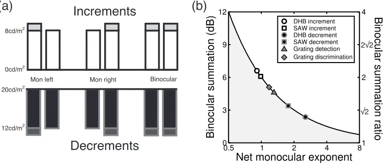
To test the prediction that there is greater summation for luminance increments, we performed a binocular summation experiment for both polarities of luminance target using the equipment and stimuli described above. Increments were on a black background (<0.01cd/m2) with a pedestal of 8cd/m2.

Decrements were relative to a bright

background (20cd/m2) with a (decrement)

pedestal of -8cd/m2. An illustration of the conditions is shown in Figure 9a. Both observers (DHB and SAW) completed four repetitions of a 2IFC luminance discrimination task in which the increments and decrements

were presented either monocularly or

binocularly against a binocular pedestal. We pooled the data across all four repetitions for each condition and estimated thresholds (75% correct) using Probit analysis. Binocular summation was calculated as the ratio of the mean monocular threshold to the binocular threshold.

The results of this experiment are shown in Figure 9b and are very clear. Summation was strong for increments, around 6dB (a ratio of 2; white filled symbols) for each observer. For

decrements, we found much weaker

(a)

(b)

Mon left Mon right Binocular

0cd/m 8cd/m

12cd/m 20cd/m

Decrements

Increments

2

2

2

2

Á2 2Á2

Figure 9. Details and results of a binocular summation experiment. (a) The conditions for a final experiment measuring binocular summation for increments and decrements. Large rectangles represent the pedestal luminances, and small ones the target increment or decrement. Each pair of bars indicates the stimulus to the left and right eyes. (b) Results from the luminance summation experiment, along with those from Meese et al. (2006) using sinusoidal grating stimuli. The curve is the level of summation expected for a range of monocular exponents, defined as BSR = 21/m, where m is the combination of all exponents prior to binocular combination (assumed to approximate a power function). Note that the curve is not a fit to the data. Rather, the data are superimposed onto the curve at x-values that permit estimation of the implied exponent from the empirical summation ratios.

5 Discussion

The purpose of this study was to investigate how target and background luminance affect

the nonlinearity underlying binocular

brightness perception. Our principal finding is that although this nonlinearity appears much stronger for decrements (Anstis & Ho, 1998) than for increments (Levelt, 1965; Engel, 1970; Anstis & Ho, 1998), a logarithmic transform of the ratio of target and background luminances removes this difference. We also demonstrate that a measure of binocular performanceÑthe binocular summation ratio for luminance excursionsÑis similarly affected by the nonlinearities that we have observed.

5.1 Alternative models

Equation 1 is a simple construct and provides a useful description of our data. It must be noted, however, that many alternative models have been proposed to account for luminance matching results (e.g. Engel, 1969; deWeert & Levelt, 1974; Lehky, 1983; Anderson & Movshon, 1989; Grossberg & Kelly, 1999). Our aim was not to compare all of these models exhaustively, since this has been attempted

elsewhere (Grossberg & Kelly, 1999).

However, we note that many such models are elaborations of equation 1, often incorporating alternative weights or additional parameters into the same basic form. The influential model of Ding & Sperling (2006, 2007) is essentially

identical to equation 1 for matching tasks at high contrast (see equation 15.27 of Ding & Sperling, 2007).

5.2 The two-stage contrast gain control model

One alternative model is the first stage of the two-stage binocular contrast gain control model of Meese, Georgeson & Baker (2006). (The second stage is an output nonlinearity, which is irrelevant to the matching paradigm.) That model was designed to explain data from

contrast detection and discrimination

experiments containing various ocular

arrangements of pedestal and target (see also, Baker, Meese & Georgeson, 2007). The equivalent expression is,

B

=

L

m

+

R

S

+

L

+

R

,

provides a good account of detection and discrimination results, including dichoptic masking, and is readily extended to incorporate cross-channel suppressive effects (e.g. Baker, Meese & Summers, 2007) as well as spatial summation (Meese & Baker, 2011).

The main departure from equation 1 is the inclusion of an extra parameter, termed S. This is typically small (S≈1 for contrasts scaled to the range 0:100), and performs a similar function to the semisaturation constant in the Naka-Rushton equation (Naka & Rushton, 1966), influencing the sensitivity of the model at low inputs. For high input levels, S has a negligible impact, and matching curves are similar to those shown in Figure 7a (see black and red curves in Figure 10). At lower input levels (where L≈R≈S), the equibrightness contours do not fold back as much when approaching either axis. This produces a summation effect at low input levels (e.g. bin > mon, see orange and green curves in Figure 10), which has been reported for previous contrast matching experiments (Legge & Rubin, 1981; Baker et al., 2007a) and is evident in some of the results here (Figures 3-5, particularly for smaller standard increments and decrements).

Figure 10: Example equibrightness contours for the two-stage model. Different colours represent different standard levels, relative to the model parameter S. When the magnitude of the standard is similar to S, there is a summation effect close to each axis. At higher input levels, the curves fold back toward the points [0, 100] and [100, 0].

5.3 Luminance matching without contours

If the difference between target and

background luminance is important, how does binocular combination behave in situations where there is no obvious background region? Using Ganzfeld (i.e. full field luminance)

stimuli, Engel (1970) found that matching behaviour was very noisy and did not produce a reliable curve. This could be due to the lack of an Ôanchor pointÕ (a region of fixed luminance) to which the target luminances could be compared (Gilchrist et al. 1999). However, Bolanowski (1989) reported linear summation of Ganzfeld brightness using a rating scale method, so obtaining successful

binocular brightness judgements from

Ganzfelds may be task dependent. Legge & Rubin (1981) performed matching experiments using full-field stimuli but not Ganzfelds, so other regions of the image (e.g. the edge of the monitor, or other objects in the room) might

have been used to anchor luminance

judgements in their study.

5.4 Separate processes for light and dark bars

In matching experiments with gratings and bipartite fields, we found that the overall nonlinearity (γ) appears to depend on the dark region of the target more than the light region (Figure 8a and inset). Based on experiments in which target gratings were deconstructed into their light and dark bars, McIlhagga & Peterson (2006) concluded that observers behave as though the light and dark parts of gratings are subject to their own luminance nonlinearities Ð the decrement nonlinearity being the more severe Ð before optimal combination. If that were the case here, then the more expansive decrement nonlinearity would be expected to

dominate at high contrasts, where its

contribution outweighs that from the

increment. This should result in a greater overall nonlinearity for contrast stimuli relative to increment-only stimuli, just as we found. Overall then, dark bars dominate over light bars for the experimental situations studied here.

5.6 Interpreting luminance nonlinearities

The benefit of the log luminance ratio is that it removes the effect of (background and target) luminance on the value of the monocular nonlinearity for the stimulus conditions here. However, as McIlhagga & Peterson (2006) point out, a realistic contrast metric should be local rather than global (though see Gilchrist et al., 1999). Considered from a biological

perspective, the luminance ratio might

1984). Indeed, a logarithmic transform may not be the only possibility - in principle, any function that is more expansive for decrements (see Figure 14 of Kingdom & Whittle, 1996) than for increments might serve our present purposes equally well. It is important to note that any nonlinearities revealed by our study must occur at a pre-binocular locus, placing them at or before primary visual cortex.

6 Conclusions

We have demonstrated that the difference between target and background luminance determines the effective nonlinearity governing binocular brightness perception. This allows experimental results for increments and decrements, which appear very different, to be understood within a single framework. We also find that the perception of binocular luminance contrast is controlled primarily by the decrement region of the stimulus. It remains to be seen whether this result is limited to binocular combination, or if it might extend to contrast perception in general.

7 Acknowledgements

Supported by BBSRC Grant BBH00159X1 and EPSRC Grant EP/H000038/1. We are grateful to Keith May for suggesting the log luminance ratio metric.

8 References

Anderson, P.A. & Movshon, J.A. (1989). Binocular combination of contrast signals. Vision Res, 29: 1115-1132.

Anstis, S. & Ho, A. (1998). Nonlinear combination of luminance excursions during flicker, simultaneous contrast, afterimages and binocular fusion. Vision Res, 38: 523-539.

Baker, D.H., Meese, T.S. & Georgeson, M.A. (2007a). Binocular interaction: contrast matching and contrast discrimination are predicted by the same model. Spat Vis, 20: 397-413.

Baker, D.H., Meese, T.S. & Summers, R.J. (2007b). Psychophysical evidence for two routes to suppression before binocular summation of signals in human vision. Neuroscience, 146: 435-448;

Bolanowski, S.J. (1987). Contourless stimuli produce binocular brightness summation. Vision Res, 27: 1943-1951.

Curtis, D.W. & Rule, S.J. (1980). FechnerÕs paradox reflects a nonmonotone relation

between binocular brightness and

luminance. Percept Psychophys, 27: 263-266.

deWeert, Ch.M.M. & Levelt, W.J.M. (1974).

Binocular brightness combinations:

additive and nonadditive aspects. Percept Psychophys, 15: 551-562.

Ding, J. & Sperling, G. (2006). A gain control theory of binocular combination. Proc Natl Acad Sci USA, 103: 1141-1146.

Ding, J. & Sperling, G. (2007). Binocular combination: measurements and a model. In Harris, L. & Jenkin, M. (eds.), Computational vision in neural and machine systems, 257-305. Cambridge University Press.

Engel, G.R. (1969). The autocorrelation function and binocular brightness mixing. Vision Res, 9: 1111-1130.

Engel, G.R. (1970). Tests of a model of binocular brightness. Can J Psychol, 24: 335-352.

Fechner, G.T. (1860). Uber einige verhŠltnisse

des binokularen sehens. Berichte sŠchs

gesmte wissenschaft, 7: 337-564.

Finney, D.J. (1971). Probit analysis.

Cambridge University Press.

Gilchrist, A., Kossifydis, C., Bonato, F., Agostini, T., Cataliotti, J., Li, X., Spehar, B., Annan, V., & Economou, E. (1999). An anchoring theory of lightness perception. Psychological Review, 106: 795-834. Grossberg, S. & Kelly, F. (1999). Neural

dynamics of binocular brightness

perception. Vision Res, 39: 3796-3816. Kingdom, F.A.A. & Whittle, P. (1996).

Contrast discrimination at high contrasts reveals the influence of local light adaptation on contrast processing. Vision Res, 36: 817-829.

Legge, G.E. & Rubin, G.S. (1981). Binocular interactions in suprathreshold contrast perception. Percept Psychophys, 30: 49-61. Legge, G.E. (1984a). Binocular contrast

summation Ð I. Detection and

discrimination. Vision Res, 24: 373-383. Legge, G.E. (1984b). Binocular contrast

summation Ð II. Quadratic summation. Vision Res, 24: 385-394.

Lehky, S.R. (1983). A model of binocular

brightness and binaural loudness

perception in humans with general

applications to nonlinear summation of sensory inputs. Biol Cybern, 49: 89-97. Levelt, W.J.M. (1965). Binocular brightness

averaging and contour information. Brit J Psychol, 56: 1-13.

MacLeod, D.I. (1972). The Schršdinger

equation in binocular brightness

McIlhagga, W. & Peterson, R. (2006). Sinusoid = light bar + dark bar? Vision Res, 46: 1934-1945.

Meese, T.S. (1995). Using the standard staircase to measure the point of subjective equality: a guide based on computer simulations. Percept Psychophys, 57: 267-281.

Meese, T.S. & Baker, D.H. (2011). Contrast summation across eyes and space is revealed along the entire dipper function by a ÒSwiss cheeseÓ stimulus. J Vis, 11(1): art. 23.

Meese, T.S., Georgeson, M.A. & Baker, D.H. (2006). Binocular contrast vision at and above threshold. J Vis, 6: 1224-1243. Naka, K.I. & Rushton, W.A. (1966).

S-potentials from colour units in the retina of fish (Cyprinidae). J Physiol, 185: 536-555. Peli, E. (1997). In search of a contrast metric:

matching the perceived contrast of Gabor patches at different phases and bandwidths. Vision Res, 37: 3217-3224.

Schršdinger, E. (1926). Die

Gesichtsempfindungen. In

Mueller-Pouillets Lehrbuch der Physik, Book 2, part 1, (11th ed., pages 456-560). Vieweg: Braunschweig.

Shapley, R.M. & Enroth-Cugell, C. (1984). Visual adaptation and retinal gain controls. Progress in retinal research, 3: 263-346. Thorn, F. & Boynton, R.M. (1974). Human

binocular summation at absolute threshold. Vision Res, 14: 445-458.

Whittle, P. (1986). Increments and decrements: luminance discrimination. Vision Res, 26: 1677-1691.