Abundance changes and habitat availability drive species’ responses to climate change

(1)

This is a repository copy of Abundance changes and habitat availability drive species’ responses to climate change.

White Rose Research Online URL for this paper: http://eprints.whiterose.ac.uk/77485/

Article:

Mair, L, Hill, J K, Fox, R et al. (3 more authors) (2014) Abundance changes and habitat availability drive species’ responses to climate change. Nature Climate Change. ISSN 1758-6798

[email protected] https://eprints.whiterose.ac.uk/ Reuse

Unless indicated otherwise, fulltext items are protected by copyright with all rights reserved. The copyright exception in section 29 of the Copyright, Designs and Patents Act 1988 allows the making of a single copy solely for the purpose of non-commercial research or private study within the limits of fair dealing. The publisher or other rights-holder may allow further reproduction and re-use of this version - refer to the White Rose Research Online record for this item. Where records identify the publisher as the copyright holder, users can verify any specific terms of use on the publisher’s website.

Takedown

If you consider content in White Rose Research Online to be in breach of UK law, please notify us by

(2)

1

Abundance changes and habitat availability drive species’ responses

1

to climate change

2

Louise Mair1, Jane K. Hill1, Richard Fox2, Marc Botham3, Tom Brereton2 & Chris D.

3

Thomas1

4

1

Department of Biology, University of York, Wentworth Way, York, YO10 5DD, UK.

5

2

Butterfly Conservation, Manor Yard, East Lulworth, Wareham, BH20 5QP, Dorset, UK.

6

3

Centre for Ecology & Hydrology, Maclean Building, Benson Lane, Crowmarsh Gifford,

7

Wallingford, Oxfordshire, OX10 8BB, UK.

8

Supplementary Information 9

Supplementary methods 10

Determinants of change in distribution area

11

The availability of distribution data was determined by the occurrence of national recording

12

efforts used to produce butterfly distribution atlases14,27. Due to the vast spatial extent of data

13

collection, annual data did not achieve sufficient spatial coverage for robust analyses and so

14

data were necessarily grouped into periods of several years. Choice of study periods were this

15

selected as 1970-82 to 1995-99 (first study period) and 1995-99 to 2005-09 (second study

16

period) corresponding to national atlas recording periods. Change in species’ distribution area

17

was calculated as the percentage change in the number of 10 km Ordnance Survey grid

18

squares with records. Sub-sampling was carried out on the distribution dataset prior to

19

analysis, to account for the large increase in recording effort over time. For example, there

20

was an increase from 185,649 records in 1970-82 to 1,710,586 records in 1995-9927.

(3)

2

sampling was carried out per 10 km grid square using an established method27, and aimed to

1

achieve a spatially and temporally consistent recording effort across Britain over time. Thus

2

for each 10 km grid square, sub-samples were taken to produce a consistent number of

3

records of each temporal resolution (records can be collected over a day, month or year) over

4

time. Sub-sampling was carried out 100 times per time period and the mean values of

5

distribution change per species obtained were used in analyses.

6

A mobility score17 was used to represent species’ dispersal ability.The mobility score was

7

determined by expert opinion from surveys17. This score was correlated with species’

8

wingspan (linear regression R2 = 0.47, P<0.001 taken from publication29) and another

9

movement index30 created using a composite of mobility variables, including some of the

10

distribution data used in this analysis (linear regression, F1,31=47.78, R2=0.59, P<0.001).

11

These relationships suggest that the mobility score from expert opinion is relatively robust.

12

Habitat availability for each species was quantified as the proportion of each species’

13

breeding habitat in the landscape using LCM200019 (for the first study period; 1970-82 to

14

1995-99) and LCM200718 (for the second study period; 1995-99 to 2005-09) 25m resolution

15

raster data. Land cover categories considered to be species’ breeding habitat were identified

16

using expert opinion14, and their importance was weighted based on the frequency with which

17

species’ distribution records were from grid squares containing that land cover type.

18

Weighting was based by computing the total number of 100 m grid square records containing

19

both the species of interest and its breeding land cover type; this value was then divided by

20

the total number of 100 m grid records of any butterfly species containing the focal species’

21

habitat land cover type. This gives a metric for the frequency of a given butterfly species in a

22

particular land cover category, relative to records of all butterfly species. Only grid cells

23

within the Ordnance Survey 100 km grid squares of the focal species’ distribution were

(4)

3

included to control for other factors limiting species’ ranges such as dispersal and climate.

1

This provided a method for weighting each land cover type in relation to the focal species’

2

use of the habitat (Table S2). The proportion of habitat available at the species’ distribution

3

leading edge (defined as the 10 km grid squares which were unoccupied at the start of the

4

study period, but colonised by the end of the study period) was estimated from land cover

5

datasets and multiplied by the species’ habitat weighting, to give an index of habitat

6

availability for each species. For species breeding in more than one habitat type, values were

7

summed across all breeding habitats to produce the index. The habitat availability index was

8

then transformed (log10) to give a normalised distribution.

9

Change in abundance was calculated using only continuously-occupied transect sites in order

10

to exclude population increases that occur following colonisation. Thus for 1995-99 to

2005-11

09, sites had to be continuously occupied by a species since 1990 to be included (1-31

12

transects per species, median = 7.6). For 1970-82 to 1995-99, the lack of early data (UKBMS

13

started in 197616) meant that sites had to be continuously occupied from 1982 to be included

14

(1-25 transects per species, median = 5). For each species, abundance trends were computed

15

from fitting mixed models by regressing log10 abundance index against year, with transect

16

site as a random variable.

17

We employed an information-theoretic approach to identify the best models for explaining

18

distribution changes in relation to abundance trends, habitat availability and dispersal ability.

19

For each of the two study periods (1970-82 to 1995-99 and 1995-99 to 2005-09), we

20

constructed general linear models to assess distribution change against all three explanatory

21

variables (habitat availability, dispersal ability and abundance change) and their interactions

22

(the literature provided evidence for linear relationships between distribution change and

23

change in abundance5, dispersal ability1 and habitat availability31, as did initial data

(5)

4

exploration). Interactions between habitat availability and dispersal might be expected if the

1

effect of habitat availability on expansion depended on the dispersal rate. Also, we might

2

expect that if abundance trends were related to change in distribution area, then positive

3

effects of habitat availability and dispersal ability might be contingent on stable or increasing

4

abundance trends. Thus all interactions between variables were explored in our analyses.

5

Explanatory variables were standardized using the function standardize in the package arm

6

(in the statistical program R28) and the function dredge in the package MuMIn was used to

7

rank models based on AICc values and Akaikes weights. Where AICc < 2, model

8

averaging was used (only models with AICc < 2 relative to the top-ranked model were

9

included in model averaging), otherwise the model with the lowest AICc value was

10

considered the best fit. Change in abundance was calculated from a different number of

11

transect sites for each species, and therefore our confidence in the estimates of this variable

12

differed among species, so we weighted species abundance trend data by the inverse of the

13

standard error of change in abundance. These analyses with weighting were then evaluated

14

against models which did not include weights, and weighting was found to be the better

15

model for distribution change in the second study period (both when species’ change in

16

abundance was computed from continuously-occupied transect sites and when it was

17

computed across all transect sites, Table S4b and d).

18

Colonisation distance distributions

19

Distributions of colonisation distances were extracted from the BNM dataset for the second

20

study period (1995-99 to 2005-09; data from the earlier period 1970-82 were of too low

21

spatial resolution and coverage for this analysis). Analyses were carried out at 1km grid

22

resolution and only colonisations occurring at species’ distribution leading edges were

23

included (defined as 10 km grid squares which were unoccupied in 1995-99 but colonised by

(6)

5

2005-09; N = 11 species, total colonisations = 12234 colonisations at 1km grid resolution,

1

14-1722 per species); colonisations occurring in 10 km grid squares where the species was

2

already present were considered to be distribution infilling and were not included in these

3

analyses.

4

Colonisation distances were extracted in R. The function ndist2 in the package splancs was

5

implemented to calculate the straight line distance from each new colony (grid square centre

6

point) in 2005-09 to the nearest existing colony (grid square centre point) present in 1995-99.

7

Records were included regardless of whether one individual or multiple individuals of species

8

were recorded. There are, however, likely to be effects of spatial and temporal variation in

9

recording effort, thus we explored different definitions of ‘existing’ and ‘new’ colonies (see

10

Fig. S1). Existing colonies can be considered to be (i) any 1 km grid square where the species

11

was recorded in 1995-99, or they can be considered to be (ii) only the 1 km grid squares

12

where the species was recorded in both 1995-99 and 2005-09. New colonies can be

13

considered to be (i) any new 1 km grid square where a species was first recorded in 2005-09,

14

or (ii) only 1 km grid squares where the species was known to be absent in 1995-99 (i.e. the

15

grid square was visited but the species was not recorded), and colonised in 2005-09.

16

We elected to present results using the most rigorous definitions, thus existing colonies were

17

those recorded in both 1995-99 and 2005-09, and new colonies were those which were visited

18

in 1995-99 but the species was not recorded present until 2005-09. Colonisation distance

19

distributions for each species were binned at 2 km intervals and fitted with an inverse power

20

function, which is a better fit than the negative exponential distribution for fat-tailed

21

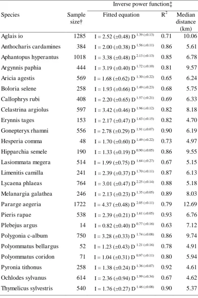
distributions33. Since colonisation kernels describe a curve rather than a single value, the

22

median distance (i.e. the distance at which the cumulative proportion of frequencies of

23

colonisation distances was 0.5) was used as a summary value of the fitted distributions (Fig 2,

(7)

6

Table S5). A multi-model inference framework was applied following the same methods as

1

outlined above for analysing distribution changes, to determine relationships between median

2

colonisation distance and habitat availability, dispersal ability and change in abundance

3

(Table S6).

4

In order to determine how our results varied according to the different definitions of existing

5

and new colonies, we extracted colonisation distance distributions using all alternative

6

combinations and applied all alternative median colonisation distances to our analyses. In

7

each case, habitat availability was found to be the most important explanatory variable, with

8

some less important positive associations shown for dispersal ability and change in

9

abundance (Table S7).This suggests that recording effort has a quantitative impact on our

10

results, but that this effect is not sufficient to change our qualitative conclusions, which

11

maintain that habitat availability is the most important variable for determining colonisation

12

distance once the expansion is taking place.

13

Phylogenetic analyses

14

In order to assess the importance of species’ phylogenetic relationships in our analyses, we

15

used AICc values and Akaike weights to compare global models incorporating phylogenetic

16

structure against global models without phylogenetic structure. A phylogenetic tree for

17

European butterflies was obtained from the literature33 and branch lengths were calculated

18

based on Grafen’s methods using the function compute.brln in the package ape in R28. The

19

phylogenetic tree was then trimmed to include only the study species. We built generalized

20

least squares (GLS) models containing all three explanatory variables and their interactions

21

(GLS models produce the same results as linear models but are directly comparable with

22

models including phylogeny), and used AICc values and Akaike weights to compare these

23

GLS models against phylogenetic generalized least squares (PGLS) models incorporating

(8)

7

phylogeny as the within-group correlation structure. We found that models incorporating

1

phylogeny had consistently higher AICc scores and lower Akaike weights than models

2

without phylogeny (Table S3), and therefore were a poorer fit to the data.

3

Phylogenetic analyses make the assumption that a phylogenetic signal is present in the data34,

4

therefore if no signal is detected it may not be appropriate to carry out phylogenetic

5

analyses35. We tested whether a phylogenetic signal was present in our dataset in order to

6

determine whether the poorer fit of the PGLS models was due to a lack of phylogenetic

7

signal. We used the pgls function in the R package caper to estimate the value of (a branch

8

length scaling parameter) using maximum likelihood. Where = 0 there is no evidence of a

9

phylogenetic signal, and where = 1 there is strong support for a Brownian model of

10

evolution34,36. We found that in all cases there was no evidence for a phylogenetic signal in

11

our data (Table S3). Detection of a phylogenetic signal is reliant on sample size as well as the

12

accuracy of the phylogenetic tree and the data37 therefore a lack of signal may be due to the

13

relatively small sample size of our dataset38 or uncertainties in Lepidoptera phylogeny.

14

Nevertheless we found no evidence that phylogenetic analyses would be appropriate or that

15

inclusion of phylogenetic correlations would produce models with a better fit to our data.

16

Thus we present data for non-phylogenetically-controlled analyses in the main text.

17

(9)

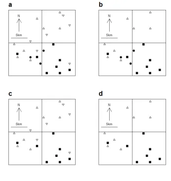
8 Supplementary figures

1

[image:9.595.121.468.113.480.2]

2

Figure S1. Schematic of different definitions of ‘existing’ and ‘new’ colonies, illustrating an

3

example of a 20 km x 20 km square area containing butterfly records at a 1km grid square

4

resolution. Existing colonies are 1 km grid squares with a species record in 1995-99 (solid

5

symbols), however these consist of those colonies which were recorded only in 1995-99

6

(solid circles), or colonies which were recorded in both 1995-99 and 2005-09 (solid squares).

7

New colonies are 1 km grid squares with a new species record in 2005-09 (open symbols),

8

and these consist of grid squares which were visited in 1995-99 and the species was not

9

recorded (upward open triangles), and grid squares which were not visited in 1995-99 so

10

previous absence of the species is not confirmed (downward open triangles). Thus the

(10)

9

available combinations of definitions are: a any existing colony (solid symbols) and any new

1

colony (open symbols), b any existing colony (solid symbols) and previously visited new

2

colonies (upward open triangles) c continuously occupied existing colonies (solid squares)

3

and any new colonies (open symbols), and d continuously occupied existing colonies (solid

4

squares) and previously visited new colonies (upward open triangles). The results of using

5

different definitions are shown in Table S7.

(11)

10 Supplementary tables

[image:11.595.68.527.205.756.2]

1

Table S1. Species’ change in distribution area, change in abundance, dispersal ability and 2

habitat availability in the first and second study period.

3

First study period (1970-82 to 1995-99) Second study period (1995-99 to 2005-09)

Species Dispersal ability* Change in distribution area (% yr-1_)‡

Change in abundance at continuously occupied sites (% yr

-1_)§

Change in abundance across all sites (% yr-1_{) §}

Habitat

availability†

Change in distribution

area (% yr-1_)‡

Change in abundance

at continuously

occupied sites (% yr-1₎

§

Change in abundance across all sites (% yr-1_{) §}

Habitat

availability†

Aglais io 39 0.55 1.06 3.30 0.039 1.71 -6.09 -2.99 0.015 Anthocharis

cardamines

32 0.65 3.80 1.52 0.080 -0.02 -4.28 -0.96 0.021

Aphantopus hyperantus

16 0.75 1.57 6.82 0.005 0.77 -2.37 2.49 0.007

Argynnis paphia 31 -1.54 0.38 0.86 0.006 1.06 6.84 3.45 0.008 Aricia agestis 12 1.06 1.27 0.82 0.007 0.61 -9.23 -5.20 0.003 Boloria

euphrosyne

18 -3.09 5.56 -3.28 0.005 - - - -

Boloria selene 19 -1.68 4.28 -2.59 0.012 -1.33 29.38 -1.91 0.014 Callophrys rubi 14 -1.53 -23.65 -0.53 0.006 0.39 -21.17 -3.35 0.014 Celastrina

argiolus

34 - - - - -0.87 -19.15 -3.58 0.017

Cupido minimus 1 -2.10 -12.62 0.41 0.001 - - - - Erynnis tages 10 -2.67 2.02 -1.04 0.003 -0.72 -53.32 -2.28 0.001 Gonepteryx

rhamni

36 -0.15 -7.23 0.26 0.035 -0.10 -2.22 -0.01 0.029

Hesperia comma

15 -0.71 10.09 13.70 0.001 3.55 -11.75 -2.07 0.001

Hipparchia semele

22 -2.41 -0.57 -2.21 0.004 -2.06 4.45 -4.09 0.002

Lasiommata megera

30 -2.24 -17.58 -4.07 0.008 -2.18 -17.59 -4.32 0.008

Limenitis camilla

27 - - - - 1.37 -4.53 -1.16 0.006

Lycaena phlaeas

26 -0.88 -3.41 0.49 0.011 -0.65 -11.54 -2.86 0.010

Melanargia galathea

24 0.61 5.50 3.81 0.008 0.03 -2.22 -2.54 0.004

(12)

11

album Polyommatus bellargus

8 -1.42 7.44 0.53 0.003 0.27 11.93 3.31 0.002

Polyommatus coridon

11 -2.04 19.30 2.41 0.004 -0.05 -5.30 -3.78 0.001

Pyronia tithonus

21 0.66 -3.50 -0.58 0.031 -0.35 -7.93 -2.85 0.020

Ochlodes sylvanus

20 -0.49 -2.65 1.61 0.028 -0.87 -19.15 -4.77 0.014

Thymelicus sylvestris

19 0.30 -6.15 0.70 0.012 -0.32 -20.37 -10.13 0.012

1

* Dispersal ability is a ranked index from expert opinion17

2

‡ Change in distribution area is the percentage change in the number of 10km grid squares

3

occupied per year (from BNM data14, see supplementary methods)

4

§ Change in abundance was calculated using BMS data15 at continuously occupied transect

5

sites (where the focal species was present every year during the study period) and across all

6

transect sites (see supplementary methods)

7

†Habitat availability from LCM 200019 and LCM200718 (see supplementary methods and

8

Table S2)

9

Missing values indicate insufficient species’ data for the species to be included in analyses

10

for that study period.

11

(13)

[image:13.595.61.536.163.756.2]

12

Table S2. Habitat availability data for each species, giving species’ scientific names and the 1

land cover category(s) which they are considered to use as breeding habitat.

2

a 1970-82 to 1995-99 3

Species Land cover category* Proportion

in

landscape†

Weight‡ Available§ Total habitat

availability¶

Aglais io 1.1 Broadleaved woodland 0.0687 0.2849 0.0195 0.0393

17.1 Suburban 0.0508 0.2810 0.0142

17.2 Urban 0.0216 0.2531 0.0054

Anthocharis cardamines

1.1 Broadleaved woodland 0.0708 0.2173 0.0153 0.0798

5.1 Improved grassland 0.2345 0.1914 0.0448

6.1 Neutral grass 0.0510 0.1655 0.0084

17.1 Suburban 0.0523 0.2125 0.0111

5.2 Setaside grass 0.0083 0.1644 0.0013 0.0050

6.1 Neutral grass 0.0486 0.0746 0.0036

Argynnis paphia

Aricia agestis 5.2 Setaside grass 0.0235 0.0835 0.0019 0.0067

6.1 Neutral grass 0.0178 0.0313 0.0005

7.1 Calcareous grass 0.0567 0.0689 0.0039

8.1 Acid grass 0.0064 0.0176 0.0001

19.1 Supra-littoral sediment 0.0015 0.1273 0.0002

Boloria euphrosyne

9.1 Bracken 0.0091 0.0260 0.0002

10.2 Open dwarf shrub heath 0.1276 0.0247 0.0031

Boloria selene 1.1 Broadleaved woodland 0.0641 0.0198 0.0012 0.0123

5.2 Setaside grass 0.0013 0.0058 0.0000

9.1 Bracken 0.0151 0.0662 0.0010

Callophrys rubi

5.2 Setaside grass 0.0092 0.0334 0.0003 0.0056

12.1 Bogs 0.0121 0.0597 0.0007

Cupido minimus

7.1 Calcareous grass 0.0632 0.0208 0.0013 0.0014

(14)

13

Erynnis tages 7.1 Calcareous grass 0.0673 0.0411 0.0027 0.0028

Gonepteryx rhamni

5.2 Setaside grass 0.0129 0.1697 0.0021

6.1 Neutral grass 0.0326 0.0719 0.0023

17.1 Suburban 0.0725 0.1651 0.0119

17.2 Urban 0.0330 0.1141 0.0037

Hesperia comma

Hipparchia semele

18.1 Supra-littoral rock 0.0003 0.3636 0.0001

Lasiommata megera

5.2 Setaside grass 0.0101 0.0446 0.0004 0.0081

8.1 Acid grass 0.0356 0.0751 0.0026

Lycaena phlaeas

5.2 Setaside grass 0.0088 0.1356 0.0012 0.0111

Melanargia galathea

5.2 Setaside grass 0.0186 0.1200 0.0022 0.0084

6.1 Neutral grass 0.0213 0.0415 0.0008

Melitaea athalia

Pararge aegeria

17.1 Suburban 0.0647 0.2266 0.0146

Pieris rapae 5.2 Setaside grass 0.0076 0.3126 0.0023 0.0324

6.1 Neutral grass 0.0554 0.2488 0.0137

17.1 Suburban 0.0470 0.3457 0.0162

Polygonia c-album

17.1 Suburban 0.0669 0.1630 0.0109

17.2 Urban 0.0292 0.1410 0.0041

Polyommatus bellargus

(15)

14

coridon

Pyronia tithonus

5.2 Setaside grass 0.0113 0.3064 0.0034 0.0307

6.1 Neutral grass 0.0357 0.1613 0.0057

17.2 Urban 0.0344 0.1814 0.0062

Ochlodes sylvanus

5.2 Setaside grass 0.0109 0.1725 0.0018

6.1 Neutral grass 0.0413 0.1213 0.0050

5.2 Setaside grass 0.0113 0.1963 0.0022 0.0120

6.1 Neutral grass 0.0395 0.1448 0.0057

8.1 Acid grass 0.0387 0.1058 0.0040

1

b 1995-99 to 2005-09 2

Species Land cover category Proportion

in

landscape

Weight Available Total habitat

availability

Aglias io 1 Broadleaved woodland 0.0349 0.2868 0.0100 0.0146

22 Urban 0.0040 0.2331 0.0009

23 Suburban 0.0127 0.2888 0.0036

Anthocharis cardamines

1 Broadleaved woodland 0.0418 0.1986 0.0083 0.0211

5 Rough grassland 0.0493 0.1572 0.0077

6 Neutral grassland 0.0034 0.2158 0.0007

23 Suburban 0.0226 0.1927 0.0043

5 Rough grassland 0.0458 0.1437 0.0065 0.0072

Argynnis paphia

Aricia agestis 5 Rough grassland 0.0285 0.0693 0.0019 0.0025

7 Calcareous grassland 0.0000 0.2272 0.0001

8 Acid grassland 0.0022 0.0239 0.0001

18 Supra-littoral sediment 0.0018 0.0597 0.0001

Boloria selene 1 Broadleaved woodland 0.0412 0.0358 0.0014 0.0139

5 Rough grassland 0.0576 0.0504 0.0029

(16)

15

Callophrys rubi

5 Rough grassland 0.0508 0.0459 0.0023 0.0140

10 Heather 0.0398 0.0833 0.0033

11 Heather grassland 0.0629 0.0761 0.0047

12 Bog 0.0348 0.0984 0.0034

Celastrina argiolus

5 Rough grassland 0.0438 0.0724 0.0031

23 Suburban 0.0425 0.1978 0.0084

Erynnis tages 7 Calcareous grassland 0.0005 0.2146 0.0001 0.0010

10 Heather 0.0194 0.0246 0.0004

Gonepteryx rhamni

5 Rough grassland 0.0388 0.136 0.0052

22 Urban 0.0189 0.1058 0.0020

23 Suburban 0.0556 0.1815 0.0100

Hesperia comma

7 Calcareous grassland 0.0075 0.0906 0.0006 0.0006

Hipparchia semele

10 Heather 0.0160 0.0494 0.0007

17 Supra-littoral rock 0.0001 0.0606 0.0001

21 Saltmarsh 0.0026 0.0208 0.0001

Lasiommata megera

5 Rough grassland 0.0520 0.0752 0.0039 0.0080

8 Acid grassland 0.0522 0.0731 0.0038

Limenitis camilla

Lycaena phlaeas

5 Rough grassland 0.0486 0.1182 0.0057 0.0095

Melanargia galathea

5 Rough grassland 0.0361 0.0953 0.0034 0.0040

(17)

16

Pararge aegeria

23 Suburban 0.0303 0.2762 0.0083

Pieris rapae 5 Rough grassland 0.0540 0.1837 0.0099 0.0161

23 Suburban 0.0174 0.3109 0.0054

Plebejus argus

10 Heather 0.0038 0.1832 0.0007 0.0016

Polygonia c-album

22 Urban 0.0111 0.1470 0.0016

23 Suburban 0.0346 0.2091 0.0072

Polyommatus bellargus

Polyommatus coridon

Pyronia tithonus

5 Rough grassland 0.0523 0.1938 0.0101 0.0202

23 Suburban 0.0467 0.1821 0.0085

Ochlodes sylvanus

5 Rough grassland 0.0479 0.1216 0.0058

5 Rough grassland 0.0482 0.1286 0.0062 0.0120

8 Acid grassland 0.0520 0.0938 0.0048

1

a the earlier study period (1970-82 to 1995-99, LCM200019)

2

b the later study period (1995-99 to 2005-09, LCM200718)

3

* land cover category numbers given refer to the class number associated with each land

4

cover category in the respective datasets

5

† the proportional area that the specific land cover type covers at the species’ distribution

6

leading edges

(18)

17

‡ calculated by dividing the number of 100m BNM records which contained both the species

1

record and their preferred land cover type, by the number of 100m BNM records (of any

2

species) that contained the land cover type

3

§ proportion of land cover type at the distribution leading edge multiplied by the weight

4

¶ the sum of ‘available’ for each species

5

Note that these land cover types are relatively coarse and hence habitat availability is a

6

relative metric and does not represent the absolute proportion of landscape that is actually

7

suitable habitat.

8

9

(19)

[image:19.595.57.533.134.528.2]

18

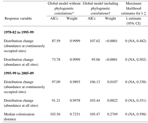
Table S3. Comparison of global models with and without phylogenetic structure using AICc 1

and Akaike weights, and maximum likelihood estimation of the parameter .

2

Global model without phylogenetic correlations*

Global model including phylogenetic

correlations†

Maximum likelihood

estimates for ‡

Response variable AICc Weight AICc Weight estimate (95% CI)

1970-82 to 1995-99

Distribution change

(abundance at continuously occupied sites)

87.59 0.9999 107.62 <0.0001 0 (NA, 0.482)

Distribution change (abundance at all sites)

73.78 0.9999 95.06 <0.0001 0 (NA, 0.502)

1995-99 to 2005-09

Distribution change

(abundance at continuously occupied sites)

97.09 0.9893 106.13 0.0107 0 (NA, 0.338)

Distribution change (abundance at all sites)

91.21 0.9978 103.44 0.0022 0 (NA, 0.351)

Median colonisation distance

103.56 0.7231 105.47 0.2769 0 (NA, 0.598)

* Generalized least squares global model with all three explanatory variables (change in

3

abundance, habitat availability and dispersal ability) and their interactions but no

4

phylogenetic structure.

5

† Phylogenetic generalized least squares global model with all three explanatory variables

6

and their interactions, and species’ phylogenetic relationships incorporated as the within

-7

group correlation structure.

(20)

19

‡ Maximum likelihood estimates for . A global model was built including phylogenetic

1

correlations with a Brownian model of evolution assumed and maximum likelihood was used

2

to estimate the value of (a branch length scaling parameter). Where = 0 there is no

3

evidence of phylogenetic signal, and where = 1 there is strong support that the trait matches

4

a Brownian model of evolution.

(21)

[image:21.595.58.506.524.742.2]

20

Table S4. Alternative general linear models assessed using an information-theoretic 1

approach.

2

a Change in distribution area (1970-82 to 1995-99, species’ change in abundance from

3

continuously-occupied transect sites only)

4

Intercept Abundance Habitat Dispersal

Abundance

x Habitat

Abundance

x dispersal

Habitat x

dispersal df logLik AICc AICc Weight Adj R2

-0.67 1.69 3 -36.9 81.0 0.00 0.480 0.35 -0.67 2.20 -0.66 4 -36.5 82.9 1.91 0.185 0.35 -0.67 0.35 1.74 4 -36.6 83.2 2.22 0.158 0.34 -0.67 0.31 2.21 -0.62 5 -36.2 85.5 4.53 0.050 0.33 -0.71 2.20 -0.65 0.25 5 -36.4 86.0 4.99 0.040 0.32 -0.67 0.33 1.74 -0.06 5 -36.6 86.4 5.37 0.033 0.31 -0.64 0.50 2.11 -0.46 0.75 6 -35.9 88.5 7.54 0.011 0.31 -0.68 0.18 2.30 -0.70 -0.49 6 -36.1 88.9 7.90 0.009 0.30 -0.71 0.31 2.21 -0.61 0.25 6 -36.1 89.0 7.96 0.009 0.30 -0.67 1.05 3 -40.9 89.0 8.02 0.009 0.11 -0.67 2 -42.9 90.3 9.34 0.004 0.00 -0.66 0.17 2.38 -0.59 -2.79 2.47 7 -34.9 90.4 9.42 0.004 0.33 -0.67 0.29 1.09 4 -40.8 91.6 10.55 0.002 0.08 -0.66 0.49 2.12 -0.46 0.72 0.11 7 -35.9 92.4 11.45 0.002 0.28 -0.75 0.14 2.31 -0.72 -0.62 0.36 7 -36.0 92.7 11.67 0.001 0.27 -0.67 0.12 3 -42.9 92.9 11.89 0.001 -0.04 -0.61 0.65 1.25 1.43 5 -40.1 93.4 12.38 0.001 0.09 -0.71 0.14 2.39 -0.61 -2.85 2.44 0.24 8 -34.9 94.8 13.75 0.000 0.30

5

6

b Change in distribution area (1995-99 to 2005-09, species’ change in abundance from

7

continuously-occupied transect sites)

8

Abundance

x Habitat

Abundance

x dispersal

Habitat x

0.23 1.43 3 -39.0 85.1 0.00 0.411 0.15 0.29 1.52 -0.36 4 -38.7 87.5 2.35 0.127 0.13 0.26 1.49 -0.30 4 -38.8 87.6 2.42 0.123 0.12 0.31 2 -41.5 87.6 2.42 0.123 0.00 0.24 1.56 -0.35 1.28 5 -38.0 89.2 4.08 0.053 0.13 0.33 -0.12 3 -41.5 90.1 4.96 0.034 -0.04 0.33 -0.10 3 -41.5 90.1 4.98 0.034 -0.04 0.22 1.65 -0.33 1.09 5 -38.5 90.2 5.03 0.033 0.10 0.29 1.53 -0.25 -0.17 5 -38.7 90.6 5.43 0.027 0.09 0.24 1.57 -0.25 -0.16 1.28 6 -38.0 92.6 7.51 0.010 0.09 0.33 -0.04 -0.10 4 -41.5 93.0 7.82 0.008 -0.09 0.25 1.68 -0.23 -0.21 1.07 6 -38.4 93.5 8.41 0.006 0.06 0.24 1.54 -0.17 -0.24 0.30 6 -38.7 94.0 8.87 0.005 0.04 0.32 -0.01 -0.12 0.09 5 -41.5 96.1 10.97 0.002 -0.14 0.25 1.50 -0.26 -0.14 1.59 -0.57 7 -38.0 96.5 11.37 0.001 0.05 0.25 1.56 -0.27 -0.14 1.30 -0.10 7 -38.0 96.6 11.43 0.001 0.05 0.22 1.68 -0.19 -0.24 1.04 0.15 7 -38.4 97.5 12.32 0.001 0.01 0.26 1.49 -0.29 -0.11 1.62 -0.58 -0.11 8 -38.0 100.9 15.77 0.000 0.00

(22)

21

c Change in distribution area (1970-82 to 1995-99, species’ abundances from all transect 1

sites)

2

Abundance

x Habitat

Abundance

x dispersal

Habitat x

-0.65 2.23 1.50 1.78 5 -27.7 68.6 0.00 0.241 0.66 -0.65 2.21 2.20 -0.86 1.56 6 -26.0 68.7 0.14 0.224 0.69 -0.70 1.77 2.28 -0.76 1.86 6 -26.4 69.4 0.80 0.161 0.68 -0.67 1.49 2.56 -1.03 5 -28.3 69.7 1.14 0.136 0.65 -0.67 1.39 1.76 4 -30.3 70.6 2.04 0.087 0.60 -0.57 2.28 2.18 -0.86 1.68 -0.40 7 -25.8 72.2 3.63 0.039 0.68 -0.57 1.87 2.24 -0.72 2.30 -0.69 7 -25.8 72.2 3.63 0.039 0.68 -0.67 2.11 2.19 -0.79 1.08 0.81 7 -25.8 72.3 3.71 0.038 0.68 -0.66 1.49 2.56 -1.03 -0.04 6 -28.3 73.2 4.65 0.024 0.63 -0.56 2.16 2.16 -0.75 0.96 1.32 -0.62 8 -25.4 75.8 7.21 0.007 0.67 -0.67 1.69 3 -36.9 81.0 12.42 0.000 0.35 -0.71 1.76 1.06 3.10 5 -34.6 82.4 13.79 0.000 0.41 -0.67 2.20 -0.66 4 -36.5 82.9 14.33 0.000 0.35 -0.67 1.25 0.97 4 -37.5 85.0 16.43 0.000 0.29 -0.71 2.20 -0.65 0.25 5 -36.4 86.0 17.41 0.000 0.32 -0.67 1.31 3 -39.7 86.5 17.93 0.000 0.19 -0.67 1.05 3 -40.9 89.0 20.44 0.000 0.11 -0.67 2 -42.9 90.3 21.76 0.000 0.00

3

4

d Change in distribution area (1995-99 to 2005-09, species’ abundances from all transect 5

sites)

6

Abundance

x Habitat

Abundance

x dispersal

Habitat x

0.09 1.26 3 -37.6 82.4 0.00 0.518 0.35 0.10 1.30 -0.28 4 -37.4 84.8 2.46 0.151 0.36 0.09 1.29 -0.18 4 -37.5 85.1 2.71 0.134 0.33 0.15 1.54 -0.29 -1.11 5 -37.1 87.3 4.92 0.044 0.33 0.10 2 -41.4 87.3 4.95 0.044 0.00 0.11 1.30 -0.29 0.02 5 -37.4 88.0 5.62 0.031 0.33 0.10 1.27 -0.17 -0.31 5 -37.5 88.2 5.81 0.028 0.31 0.10 0.06 3 -41.4 89.9 7.53 0.012 -0.04 0.10 -0.05 3 -41.4 89.9 7.54 0.012 -0.04 0.15 1.54 -0.33 0.07 -1.13 6 -37.1 90.8 8.42 0.008 0.30 0.11 1.29 -0.28 0.02 -0.24 6 -37.4 91.5 9.09 0.005 0.30 0.09 1.30 -0.26 0.00 0.10 6 -37.4 91.5 9.12 0.005 0.30 0.11 -0.15 0.17 4 -41.4 92.7 10.34 0.003 -0.09 0.15 1.65 -0.38 0.09 -1.55 0.65 7 -37.0 94.6 12.17 0.001 0.27 0.11 1.53 -0.25 0.02 -1.18 0.26 7 -37.0 94.7 12.29 0.001 0.26 0.09 1.28 -0.23 -0.01 -0.27 0.16 7 -37.4 95.4 13.00 0.001 0.27 -0.01 0.06 0.03 0.72 5 -41.2 95.6 13.20 0.001 -0.14 0.12 1.64 -0.32 0.06 -1.56 0.61 0.19 8 -37.0 98.9 16.55 0.000 0.23

7

a distribution change in the first study period (1970-82 to 1995-99, using species’ change in 8

abundance at continuously-occupied transect sites)

(23)

22

b distribution change in the second study period (1995-99 to 2005-09, using species’ change 1

in abundance at continuously-occupied sites only)

2

c distribution change in the first study period (using species’ change in abundance across all 3

transect sites)

4

d distribution change in the second study period (using species’ change in abundance across

5

all transect sites)

6

Variable estimates are given, along with the log likelihood, AICc value, difference in AICc

7

between the top model and all other models ( AICc), Akaike weights and the adjusted R

-8

squared value for each model. Models are ordered starting with the best fit.

9

(24)

[image:24.595.70.461.137.724.2]

23

Table S5. Summary data for colonisation distance distributions for each species for the 1

second study period (1995-99 to 2005-09).

2

Inverse power function‡

Species Sample

size†

Fitted equation R2 Median distance (km) Aglais io 1285 I = 2.52 (±0.48) D 1.39 (±0.13) 0.71 10.06

Anthocharis cardamines 384 I = 2.00 (±0.38) D 1.56 (±0.11) 0.86 5.61

Aphantopus hyperantus 1018 I = 3.38 (±0.48) D 2.13 (±0.13) 0.85 6.78

Argynnis paphia 444 I = 3.19 (±0.40) D 1.72 (±0.10) 0.81 9.57

Aricia agestis 569 I = 1.68 (±0.62) D 1.30 (±0.22) 0.65 6.24

Boloria selene 258 I = 1.93 (±0.66) D 1.49 (±0.23) 0.68 5.75

Callophrys rubi 408 I = 2.20 (±0.65) D 1.57 (±0.21) 0.69 6.33

Celastrina argiolus 597 I = 3.42 (±0.46) D 1.96 (±0.12) 0.82 8.18

Erynnis tages 153 I = 2.17 (±0.47) D 1.63 (±0.15) 0.82 4.70

Gonepteryx rhamni 556 I = 2.78 (±0.29) D 1.91 (±0.07) 0.90 6.19

Hesperia comma 48 I = 1.70 (±0.60) D 1.49 (±0.22) 0.73 4.97

Hipparchia semele 190 I = 1.33 (±0.19) D 0.90 (±0.05) 0.86 9.55

Lasiommata megera 514 I = 1.99 (±0.75) D 1.64 (±0.27) 0.67 5.15

Limenitis camilla 241 I = 2.39 (±0.37) D 1.70 (±0.11) 0.87 6.13

Lycaena phlaeas 764 I = 3.01 (±0.47) D 2.25 (±0.14) 0.88 5.18

Melanargia galathea 246 I = 2.13 (±0.23) D 1.35 (±0.05) 0.89 8.03

Pararge aegeria 1722 I = 4.37 (±0.48) D 2.05 (±0.11) 0.79 12.69

Pieris rapae 538 I = 2.39 (±0.21) D 1.61 (±0.05) 0.93 6.76

Plebejus argus 14 I = 0.82 (±0.40) D 0.77 (±0.16) 0.63 7.12

Polygonia c-album 750 I = 3.28 (±0.33) D 1.74 (±0.08) 0.86 9.74

Polyommatus bellargus 52 I = 1.23 (±0.43) D 1.21 (±0.16) 0.78 4.91

Polyommatus coridon 71 I = 1.04 (±0.31) D 0.97 (±0.11) 0.80 5.94

Pyronia tithonus 258 I = 1.38 (±0.24) D 1.36 (±0.07) 0.92 4.61

Ochlodes sylvanus 614 I = 2.36 (±0.94) D 1.99 (±0.34) 0.67 4.62

Thymelicus sylvestris 540 I = 1.76 (±0.27) D 1.46 (±0.08) 0.90 5.37

(25)

24

† sample size is number of new 1 km colonies included in analysis

1

‡ the fitted inverse power function equation with the R-squared value indicating the fit of the

2

function to the raw data and the median colonisation distance from the fitted equation

3

Total sample size = 12234 colonisations at the 1 km resolution.

4

5

6

(26)

[image:26.595.63.527.137.353.2]

25

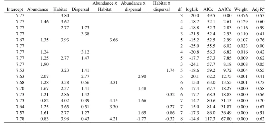
Table S6. Alternative general linear models assessed using an information-theoretic approach 1

for species’ median colonisation distance in the later study period (1995-99 to 2005-09).

2

Abundance x

Habitat

Abundance x

dispersal

Habitat x

7.77 3.80 3 -20.0 49.5 0.00 0.476 0.55 7.77 1.46 3.62 4 -18.7 52.1 2.61 0.129 0.60 7.77 2.77 1.73 4 -18.8 52.3 2.83 0.116 0.59 7.77 3.38 3 -21.5 52.4 2.93 0.110 0.41 7.67 1.35 3.93 3.66 5 -15.2 52.5 2.99 0.107 0.76

7.77 2 -25.0 55.5 6.02 0.023 0.00

7.77 1.24 3.12 4 -20.8 56.3 6.82 0.016 0.42 7.77 1.25 2.77 1.47 5 -17.7 57.3 7.85 0.009 0.62 7.77 1.90 3 -24.1 57.7 8.18 0.008 0.05 7.53 3.23 1.41 1.74 5 -18.6 59.2 9.72 0.004 0.55 7.63 2.07 2.77 2.90 5 -20.1 62.2 12.75 0.001 0.41 7.68 1.28 3.58 0.56 3.31 6 -15.0 63.0 13.55 0.001 0.73 7.70 1.67 2.57 1.41 1.48 6 -17.4 67.7 18.27 0.000 0.58 7.73 1.21 2.86 1.42 0.32 6 -17.7 68.3 18.83 0.000 0.56 7.73 0.82 4.02 0.39 4.15 -1.66 7 -14.7 80.6 31.15 0.000 0.70 7.64 1.25 3.65 0.51 3.30 0.27 7 -15.0 81.4 31.87 0.000 0.67 7.57 1.61 2.77 1.27 1.65 0.86 7 -17.3 86.0 36.49 0.000 0.51 7.78 0.83 3.96 0.43 4.21 -1.77 -0.32 8 -14.6 117.3 67.80 0.000 0.62

3

Variable estimated are given, along with thelog likelihood, AICc value, difference in AICc

4

between the top model and all other models ( AICc), Akaike weights and the adjusted r

-5

squared value for each model. Models are ordered starting with the best fit.

6

(27)

26

Table S7. Average model parameter estimates, standard errors and relative variable 1

importance for median colonisation distance using different definitions of existing and new

2

colonies.

3

4

5

6

7

8

9

10

11

12

13

a any existing and any new colonies (SI Fig 1a) 14

b any existing and previously visited new colonies (SI Fig 1b) 15

c continuously occupied existing colonies and any new colonies (SI Fig. 1c) 16

* Relative importance of variables of 1 indicates that the variable was present in all top

17

models, or was the only variable when model averaging was not necessary because the

18

difference in AICc between the first and second highest ranking models was > 2.

19

20

Best-fit model variables Estimate Unconditional S.E.

Relative variable importance*

(a) Using any existing and any new

Habitat availability 3.441 0.857 1

Change in abundance 1.372 0.668 0.62

Habitat x abundance 4.414 1.272 0.62

(b) Any existing and previously visited new

Habitat availability 3.319 1.023 0.79

Change in abundance 1.445 0.783 0.43

Habitat x abundance 5.074 1.492 0.43

Dispersal ability 2.975 1.291 0.21

(c) Continuously occupied existing and any new

Habitat availability 3.776 1.143 1

(28)

27 Supplementary References

1

29 Sekar, S. A meta-analysis of the traits affecting dispersal ability in butterflies: can

2

wingspan be used as a proxy? J. Anim. Ecol. 81, 174-184 (2012).

3

30 Dennis, R. L. H. & Shreeve, T. G. Butterflies on British and Irish offshore islands.

4

(Gem Publishing Company, 1996).

5

31 Hill, J. K. et al. Impacts of landscape structure on butterfly range expansion. Ecology

6

Letters 4, 313-321 (2001).

7

32 Chapman, D. S., Dytham, C. & Oxford, G. S. Modelling population redistribution in a

8

leaf beetle: an evaluation of alternative dispersal functions. J. Anim. Ecol. 76, 36-44

9

(2007).

10

33 Cizek, O. & Konvicka, M. What is a patch in a dynamic metapopulation? Mobility of

11

an endangered woodland butterfly, Euphydryas maturna. Ecography 28, 791-800

12

(2005).

13

34 Hernández, C. E. et al. Using phylogenetic information and the comparative method

14

to evaluate hypotheses in macroecology. Methods in Ecology and Evolution 4,

401-15

415 (2013).

16

35 Ashton, K. G. Comparing phylogenetic signal in intraspecific and interspecific body

17

size datasets. Journal of Evolutionary Biology 17, 1157-1161 (2004).

18

36 Pagel, M. Inferring the historical patterns of biological evolution. Nature 401,

877-19

884 (1999).

20

37 Blomberg, S. P., Garland, T. & Ives, A. R. Testing for phylogenetic signal in

21

comparative data: behavioural traits are more labile. Evolution 57, 717-745 (2003).

22

38 Freckleton, R. P., Harvey, P. H. & Pagel, M. Phylogenetic analysis and comparative

23

data: A test and review of evidence. The American Naturalist 160, 712-726 (2002).