Control of Production-Distribution Systems under Discrete
Disturbances and Control Actions
Dario Bauso and Danielle C. Tarraf
Abstract— This paper deals with the robust control and optimization of production-distribution systems. The model used in our problem formulation is a general network flow model that describes production, logistics, and transportation applications. The novelty in our formulation is in the discrete nature of the control and disturbance inputs. We highlight three main contributions: First, we derive a necessary and sufficient condition for the existence of robustly control in-variant hyperboxes. Second, we show that a stricter version of the same condition is sufficient for global convergence to an invariant set. Third, for the scalar case, we show that these results parallel existing results in the setting where the control actions and disturbances are analog. We conclude with two simple illustrative examples.
I. INTRODUCTION
By production-distribution systems we mean any system where resources at geographically distributed warehouses are converted into products with (in the case of production) or without (in the case of distribution) physical modifications of the goods, commodities, materials involved in the process. In this sense, the term is quite general, encompassing both production and logistics models.
Production-distribution systems can be thought of as net-work flow problems, as they are efficiently described using graphs or hypergraphs with nodes and arcs associated with resources/products and flows, respectively. The accumulated discrepancy over time of the input and output flows at n interconnected nodes is captured by the n-dimensional state of the system: Practically, this represents resources and or products available (stored) at thenwarehouses. The control input denotes the controlled flows (i.e. the production and/or distribution) and the disturbance input denotes the uncontrolled flows (i.e. the demand). The dynamics of the system are thus linear, with the matrices defining the model describing which and in what quantity resources and products are involved in a unit flow.
Practically, resource/product inventory stored at the ware-houses translate into holding costs for the warehouse man-ager, and so one desires to keep the inventory bounded and as close as possible to the unknown demand. On the other hand, keeping the inventory close to zero may induce shortages and subsequent loss of clients for the warehouse manager, hence there is a tradeoff. Questions of existence of robustly control invariant sets, as well as their properties when they do
D. Bauso is with Dipartimento di Ingegneria Chimica, Gestionale, Informatica e Meccanica, Universit`a di Palermo, Italy ([email protected]).
D. C. Tarraf is with the Department of Electrical and Computer Engineering, Johns Hopkins University, Baltimore, MD 21218, USA ([email protected]).
exist, are thus of interest. Of course, this problem has been previously considered in the literature, for instance in [6] [7] where polytopic invariant sets as considered and in [5] where ellipsoidal sets are considered. Restricting the discussion to polytopic sets has the advantage of reducing the problem to linear programs, with the relative computational benefits: The problem turns into a robust quadratic programming problem involving linear matrix inequalities when the sets are ellipsoidal.
The novelty of this paper is in the discrete nature of the inputs, justifiable from practical as well as theoretical perspectives. From a practical standpoint, materials and goods are usually processed in batches. From a theoretical standpoint, the study of systems under discrete controls and disturbances has sparked much interest in recent years as evidenced by the literature on alphabet control [8] [9], [10], mixed integer model predictive control [1], discrete team theory [11] and boolean control [3]. In general, the problems of interest may be formulated as min-max games [2].
Our contribution consists of three main results. First, we derive a necessary and sufficient condition for the existence of robustly control invariant hyperboxes. Second, we show that a stricter version of the above condition is sufficient to guarantee global convergence of all state trajectories to the invariant set. Finally, we show that these two results when specialized to the scalar case share striking similarities to existing results in the literature where the inputs are assumed to be analog [6] [7].
The paper is organized as follows: We formulate the problem in Section II. We state and prove the main results in Section III, and we discuss their specialization for the scalar case in the context of existing work. We present two simple illustrative examples in Section IV and conclude in Section V.
A word on notation: R and Z denote the set of reals
and integers, respectively. [x]i denotes the ith component
of vector x∈ Rn. hull{S} and int(S) denote the convex
hull and interior, respectively, of setS⊂Rn.Bndenotes the
set of vertices of the unit hypercube, that isBn ={0,1}n.
II. SETUP OF THE PROBLEM
A. Problem Statement
Consider the system described by
x(t+ 1) =x(t) +Bu(t)−Dw(t) (1) where time index t ∈ Z+, state x(t) ∈ Rn, control input
u(t)∈ Um and disturbance input w(t)∈ Wp. The control
a1< . . . < ar. Likewise the disturbance alphabet set W =
{b1, . . . , bq} is a discrete ordered set with b1 < . . . < bq.
Matrices B ∈ {−1,0,1}n×m and D ∈ {−1,0,1}n×p are
given.
Definition 1: A set X = [0, x+1]×. . .×[0, x+
n] ⊂ Rn,
x+i >0, is robustly control invariant if there exists a control law ϕ : X → Um such that for every x(t) ∈ X, x(t+
1) = x(t) +Bϕ(x(t))−Dw(t) ∈ X for any disturbance w(t)∈ Wp.
Remark 1: WhenX = [0, x+1]×. . .×[0, x+
n]is robustly
control invariant, then so is any other hyperbox X0 = [x−1, x−1 +x+1]×. . .×[x−n, x−n +x+n]. Indeed, control law
ϕ0 : X0 → Um defined by ϕ0(x) = ϕ(x−x−), where
[x−]i=x−i , verifies this assertion.
Definition 2: A robustly control invariant set X = [0, x+1]×. . .×[0, x+n] ⊂ Rn is globally attractive if there
exists a control law ψ : Rn \ X → Um such that for
every initial condition x(0) ∈ Rn \ X and disturbance
w:Z+→ Wp, there exists aτ∈Z+ such thatx(τ)∈X.
We are interested in answering two questions for this class of systems:
Question 1:Under what conditions does a robustly control invariant setX exist?
Question 2: Under what conditions is a robustly control invariant setX globally attractive?
B. Significance of the Problem Statement
Dynamics (1) describes the evolution of production-distribution systems where the statex(t)represents resources and or products available (stored) at the n warehouses, the control input u(t) denotes the controlled (production-distribution) flows and the disturbance input w(t) the un-controlled flows. Matrix B establishes which and in what quantity resources and products are involved in a unit flow. Observe that depending on the sign of theijth entry inBthe samexi is a resource (negative sign) or a product (positive
sign) for flowj.
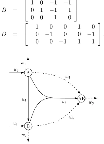
An efficient way to describe production-distribution sys-tems is by using hypergraphs with nodes and arcs associated to resources/products and flows respectively. For the example in Fig. 1 borrowed from [7], we have three resourses/products xi, i = 1,2,3, four controlled flows ui, i = 1, . . . ,4 and
five uncontrolled flowswi,i= 1, . . . ,5. One unit of flowu1 produces one unit of product A associated tox1. Same for flow u2 and product B associated to x2. One unit of flow u3 uses one unit of resources A and B to produce one unit of product AB associated to x3. One unit of flow u4 uses one unit of resources A to produce one unit of product B. Similar explanation for the uncontrolled flows with the only exception that these are exogenously set. So, one unit of flow w1 is a unitary demand of resource A, and similarly forw2 andw3 with resource B and AB respectively. Floww4uses
A to produce AB as well asw5 uses B to produce AB. The highlighted relations between flows and resources/products are described by matrices
B =
1 0 −1 −1
0 1 −1 1
0 0 1 0
D =
−1 0 0 −1 0
0 −1 0 0 −1
0 0 −1 1 1
.
A
B
AB
u1
u2 u4
u3 w4
w5 w3
[image:2.612.350.518.100.332.2]w2 w1
Fig. 1. Network system with three resourses/products, four controlled (solid) and five uncontrolled (dashed) flows.
From the example, the motivation of looking at the smallest robustly controlled invariant set is clear. Since resource/product inventory stored at the warehouse translate into holding costs for the warehouse manager, we may want to keep the inventory bounded and as close as possible to the expected demand (uncontrolled flows), this one being unknown. At the same time, keeping the inventory close to zero may induce shortages (lost of clients) for the warehouse manager. One practical way to deal with robustly controlled invariant set is to apriori impose some structure and restrict the search to polytopic or ellipsoidal sets (cfg. [4], [5], [6], [7]). The simplicity with which these sets can be formulated translates into computational tractability for the optimization problems involved in the study (linear or quadratic mathe-matical programs).
III. MAIN RESULTS
Consider the following sets fori∈ {1, . . . , n} Ui
+ = {u∈ U
m|[Bu−Dw]
i≥0,∀w∈ Wp}
Ui
− = {u∈ Um|[Bu−Dw]i≤0,∀w∈ Wp}
Ui
+∗ = {u∈ Um|[Bu−Dw]i>0,∀w∈ Wp}
Ui
−∗ = {u∈ Um|[Bu−Dw]i<0,∀w∈ Wp},
associate with everyx∈Rn
+ asignature, namely an n-tuple
(s1, . . . , sn)withsi= +if[x]i = 0andsi=−if[x]i>0,
and two subsets ofUm defined by
Ux=Us11∩. . .∩ U
n sn, Ux∗=U1
s1∗∩. . .∩ U
A. Existence of a Robustly Control Invariant Set
Theorem 1: The following two statements are equivalent:
(a) There exists a setX = [0, x+1]×. . .×[0, x+n] that is robustly control invariant.
(b) The condition
Uz6=∅ (2)
holds for all z∈Bn.
Proof: (a)⇒(b): Assume thatUz=∅for somez∈Bn
with signature (s1, . . . , s2). Consider a set X = [0, x+1]× . . .×[0, x+n],x
+
i >0, and au∈ U
m. By assumption, there
exists an i ∈ {1, . . . , n} such that u /∈ Ui
si. Now pick the vertexxof X given by
[x]j=
0 s
j = +
x+j sj =−
Note that the signatures ofzandxare identical by construc-tion. Lettingx(t) =xand applying control inputu(t) =u, we have
[x(t+ 1)]i= [x(t) +Bu(t)−Dw(t)]i= [x]i+ [Bu−Dw]i,
and[x(t+ 1)]i−[x(t)]i= [Bu(t)−Dw(t)]i satisfies
[x(t+ 1)]i−[x(t)]i>0
for somew∈ Wp when [x]
i6= 0 and
[x(t+ 1)]i−[x(t)]i<0
for some w ∈ Wp when [x]
i = 0. Hence x(t+ 1) ∈/ X
for somew∈ Wp. Noting that the choice ofuwas arbitrary
allows us to conclude thatXis not robustly control invariant. Noting that the choice of X was arbitrary allows us to conclude that a robustly control invariant set cannot exist, thus completing our argument.
(b)⇒(a): The proof is constructive. Assume thatUz6=∅
holds for allz∈Bn, and pickuz∈ Uz. Define
L∗i = max
w,z
[Buz−Dw]i
The set X = [0,2L∗1]×. . .×[0,2L∗n] is robustly control invariant. Indeed, consider the control law ϕ : X → Um
defined by ϕ(x) = uz(x), where z(x) ∈ Bn is the unique
vertex of the unit hypercube with signaturesi = +if[x]i ≤
L∗
i andsi =−otherwise. Note that under this control law,
we have for anyi∈ {1, . . . , n}
[x(t+ 1)]i= [x(t)]i+ [Bϕ(x(t))−Dw(t)]i
Thus by construction, when 0 ≤ [x(t)]i ≤ L∗i, 0 ≤
[Bϕ(x(t))−Dw(t)]i ≤ Li∗ and 0 ≤ [x(t+ 1)]i ≤ 2L∗i.
Likewise when Li <[x(t)]i ≤ 2Li∗, −L∗i ≤ [Bϕ(x(t))−
Dw(t)]i ≤0 and 0≤[x(t+ 1)]i≤2L∗i. It follows that X
is robustly control invariant.
B. Global Attractiveness
Theorem 2: If condition
Uz∗6=∅ (3)
holds for all z ∈ Bn, there exists a set X = [0, x+1]× . . .×[0, x+n] that is robustly control invariant and globally attractive.
Proof: The proof is constructive. For eachz∈Bn, pick
uz∈ Uz∗. Define
L∗i = max
w,z
[Bu(z)−Dw]i
The set X = [0,2L∗1]×. . .×[0,2L∗n] is robustly control invariant and globally attractive. Indeed, consider the control law ζ :Rn → Um defined byζ(x) =uz(x), where z(x)∈
Bnis the unique vertex of the unit hypercube with signature
si = + if [x]i ≤ L∗i and si = − otherwise. Noting that
U∗
z ⊆ Uz, it immediately follows thatX is robustly control
invariant by a proof identical to the proof of sufficiency in Theorem 1. To prove global attractiveness, let
∆ = min
i minz,w
[Buz−Dw]i
and consider the functionV :Rn →Rdefined by
V(x) = max
i miny∈X
[x]i−[y]i . Note that by construction, we have:
• ∆>0.
• V(x)≥0, for allx∈Rn.
• V(x) = 0⇔x∈X.
When control law ζ is utilized, we can show that along system trajectories, we have
V(x(t+ 1))−V(x(t))<0 (4)
whenever x(t) ∈ Rn \ X. The details are omitted here,
but the idea is to appropriately partition the state-space into polytopes in which this inequality can be verified. Moreover, we have
V(x(t+ 1))≤V(x(t))−∆ (5)
whenever x(t)∈Rn\X andx(t+ 1)∈Rn\X.
Thus, for any choice of initial condition x(0) and of disturbance input w : Z+ → Wp, we conclude from (4) that lim
t→∞V(x(t)) → 0. Moreover, we conclude from (5)
that there must exist a τ > 0 such that V(x(τ)) = 0, or equivalently x(τ) ∈ X. Hence X is indeed globally attractive.
C. Interpretation of the Main Results in the Scalar Case
In this section, we consider the special case of scalar dynamics in order to point out that Theorem 1 is strikingly parallel to existing results for the setup where the control and disturbance are assumed to take continuous values.
Consider the dynamics described by
where α and η are given non-zero scalars, u(t) ∈ U and w(t)∈ W.
The relevant sets can be computed by looking at the signs of the entries of the following table
u/w b1 . . . bq
a1 αa1−ηb1 . . . αa1−ηbq
..
. ... ...
ar
Specifically, we have the following subsets of U:
U+ = {u∈ U |αu−ηw≥0,∀w∈ W}
U− = {u∈ U |αu−ηw≤0,∀w∈ W}
U+∗ = {u∈ U |αu−ηw >0,∀w∈ W}
U−∗ = {u∈ U |αu−ηw <0,∀w∈ W}
Note thatU+∗⊆ U+ andU−∗⊆ U−.
Lemma 1: U+ 6= ∅ and U− 6= ∅ iff hull{ηW} ⊆ hull{αU }.
Proof: To prove sufficiency, assume that one of the two sets, sayU+, is empty. Thus for everyu∈ U, there exists a w ∈ W such that αu−ηw <0. In particular, there exists w∈ W such thatαam−ηw <0, equivalently ηw > αam,
and hence there exists an elementy∈hull{ηW} such that y /∈hull{αU }.
To prove necessity, assume that U+ 6= ∅ and U− 6= ∅.
Thus there existsu1∈ U+ andu2∈ U− satisfying
αu1−ηw≥0 αu2−ηw≤0
for allw∈ W. Since am≥u1 anda1≤u2, we have
αam−ηw≥0
αa1−ηw≤0
⇔
αam≥ηw
αa1≤ηw
for all w ∈ W. In particular, it holds that αam≥ηbp and
αa1≤ηb1hence hull{ηW} ⊆hull{αU }.
Corollary 1: The following two statements are equivalent: 1) There exists a finite set X = [0, x+] that is robustly
control invariant. 2) hull{ηW} ⊆hull{αU }.
Proof: Noting that condition (2) is equivalent to the condition U+ 6= ∅ and U− 6= ∅ in the scalar setting,
the statement of the corollary follows from Lemma 1 and Theorem 1.
Remark 2: The statement of Corollary 1 reminds us of the well known set dominance conditions provided in [7] for the discrete-time flow model with continuous inputs. The use of the hull(.) operator is made necessary as in our case the alphabet setsU andW are discrete sets rather than polytopes as in [7]. Similar conditions have been shown to play the same important role also in [6] for the continuous-time version: Future work will investigate the relevance of these conditions for the case of continuous time system with discrete control and disturbance alphabets
Lemma 2: SupposeU+6=∅ andU−6=∅. We have
U+∗6=∅ orU−∗6=∅ ⇔hull{ηW} ⊂hull{αU }.
Proof: To prove sufficiency, assume thathull{ηW} ⊂
hull{αU }. Thus there exists at least one element x in hull{αU }and not inhull{ηW}. Ifxis strictly larger than every element inhull{ηW}, thenαamis also strictly larger
than every element in hull{ηW}, αam−ηw > 0 for all
w ∈ W, am ∈ U+∗, and U+∗ 6= ∅. Otherwise, x must be
strictly smaller than every element inhull{ηW}, and by a similar argumentU−∗ 6=∅.
To prove necessity, assume that U+∗ 6= ∅ or U−∗ 6= ∅.
If there exists u1 ∈ U+∗ satisfying αu1−ηw > 0 for all w ∈ W, then since am ≥u1 we have αam−ηw > 0 ⇔
αam> ηwfor allw∈ W. In particular it holds thatαam>
ηbp, hence hull{ηW} ⊂ hull{αU }. Otherwise there must
exist a u2 ∈ U−∗ satisfying αu2−ηw <0 for allw∈ W. Since a1 ≤ u2, we have αa1−ηw < 0b ⇔ αa1 < ηw, for allw∈ W. In particular it holds αa1 < ηb1 and hence hull{ηW} ⊂hull{αU }.
IV. ILLUSTRATIVE EXAMPLES
A. A Scalar System
Let us start with a scalar example. Consider dynamics (6) and take inputs u ∈ U = {−100,−2,3,150}, w ∈ W = {−6,4}, and parameters α=η = 1. We first compute the relevant sets by direct inspection of the table below:
u/w −6 4 −100 −94 −104
−2 4 −6
3 9 −1
150 156 146
We have U+ =U+∗ ={150} and U− =U−∗ ={−100}.
Invoking Theorems 1 and 2, we conclude that a robustly control invariant set exists, and moreover it is globally attractive. Indeed, it is easy to verify that the setX= [0,157]
is one such set (in fact, the smallest!).
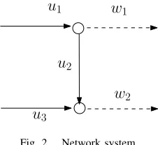
B. Network with 2 Nodes
u
1u
2u
3w
1 [image:4.612.379.492.556.660.2]w
2Fig. 2. Network system.
flowsu1andu2represent the exogenous demand of resource x1andx2 respectively. The associated dynamics are then:
x1(t+ 1) x2(t+ 1)
=
x1(t) x2(t)
+
1 −1 0
0 1 1
u1(t) u2(t) u3(t)
−
w1(t) w2(t)
Assume that flows can only be processed in batches withU = {−5,−2,1,6}, and the disturbances also appear in batches withW={−3,2}.
We begin by computing the relevant sets:
U1
+ = {(−2,−5,x),(1,−5,x),(1,−2,x),(6,−5,x),
(6,−2,x),(−6,1,x)} U1
− = {(−5,−2,x),(−5,1,x),(−5,6,x),(−2,1,x),
(−2,6,x),(1,6,x)} U2
+ = {(x,−2,6),(x,1,1),(x,1,6),(x,6,−2),
(x,6,1),(x,−6,6)}
U−2 = {(x,−5,−5),(x,−5,−2),(x,−5,1),(x,−2,−5),
(x,−2,−2),(x,1,−5)}
Note that, for instance, we write (−2,−5,x) to mean any control vector with u1 = −2 and u2 = −5. Note that condition (2) holds. Indeed,
u1 = (1,−2,6)∈U+1∩U+2 u2 = (1,−2,−5)∈U+1 ∩U−2, u3 = (−5,1,−5)∈U−1 ∩U−2, u4 = (−5,1,6)∈U−1∩U+2.
Invoking Theorem 1, we look for a robustly controlled invariant set. To do this, following the proof of Theorem 1, we first need to calculate setsLji which take on the following values:
L11= max
w |1 + 2−w|= 6, L
3
1= maxw | −5−1−w|= 8 L12= max
w | −2 + 6−w|= 7, L
3 2= max
w |1−5−w|= 6
L21= max
w |1 + 2−w|= 6, L
4
1= maxw | −5−1−w|= 8 L22= max
w | −2−5−w|= 9, L
1
2= maxw |1 + 6−w|= 10
Then, we need to look for the maximal valuesL∗i which yield
L∗1 = max
j {L j
1}j= max{6,6,8,8}= 8
L∗2 = max
j {L j
2}j= max{7,9,6,10}= 10.
We can then conclude (see Remark 1) that the following setX is robustly control invariant:
X ={x∈R2| −8≤x1≤8,−10≤x2≤10}.
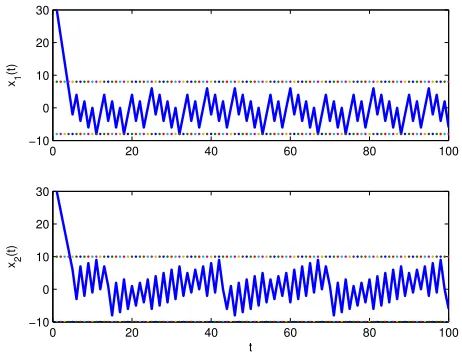
In Fig. 3, we plot the evolution of x1(t) and x2(t) for t= 1, . . . ,100with initial statex(0) = [30 30]T. The plot
shows that the statex(t)converges toX ={x∈R2| −8≤
x1≤8, −10≤x2≤10}.
0 20 40 60 80 100
−10 0 10 20 30
x1
(t)
0 20 40 60 80 100
−10 0 10 20 30
x2
(t)
[image:5.612.320.551.126.303.2]t
Fig. 3. Time plot ofx1(t)andx2(t)fort= 1, . . . ,100: in evidence the
global convergence ofx(t)toX ={x∈R2| −8≤x
1 ≤8,−10≤
x2≤10}.
V. CONCLUSIONS AND FUTURE WORK
In this paper we have provided a detailed analysis of existence conditions of robustly controlled invariant sets for production-distribution systems. The original aspect of the paper lies in the discrete nature of the control and disturbance inputs. Connections with existing results in the setup where the inputs are continuous are emphasized.
Our future research will focus on deriving bounds for the smallest invariant set, interpreting the derived necessary and sufficient conditions in the context of existing results for the general case, considering other models of discrete uncertainty, and revisiting the problem for continuous time dynamics.
VI. ACKNOWLEDGMENTS
D. C. Tarraf’s research was supported by NSF CAREER award ECCS 0954601 and AFOSR YIP award FA9550-11-1-0118.
REFERENCES
[1] D. Axehill, L. Vandenberghe, and A. Hansson. Convex relaxations for mixed integer predictive control. Automatica, 46(5):1540–1545, June 2010.
[2] T. Basar and G.J. Olsder. Dynamic Noncooperative Game Theory. SIAM, 1999.
[3] D. Bauso. Boolean-controlled systems via receding horizon and linear programming. Journal of Mathematics of Control, Signals and Systems, 21(1):69–91, 2009.
[4] D. Bauso, F. Blanchini, and R. Pesenti. Optimization of long-run average-flow cost in networks with time-varying unknown demand. IEEE Trans. on Automatic Control, 55(1):20–31, 2010.
[6] F. Blanchini, S. Miani, and W. Ukovich. Control of production-distribution systems with unknown inputs and system failures. IEEE Trans. on Automatic Control, 45(6):1072–1081, 2000.
[7] F. Blanchini, F. Rinaldi, and W. Ukovich. Least inventory control of multi-storage systems with non-stochastic unknown input. IEEE Trans. on Robotics and Automation, 13(5):633–645, 1997.
[8] G. C. Goodwin and D. E. Quevedo. Finite alphabet control and estimation.International Journal of Control, Automation and Systems, 1(4):412–430, 2003.
[9] D. C. Tarraf, A. Megretski, and M. A. Dahleh. Finite approximations of switched homogeneous systems for controller synthesis. IEEE Transactions on Automatic Control, 56(5):1140–1145, May 2011. [10] D.C. Tarraf, A. Megretski, and M.A. Dahleh. A framework for robust
stability for systems over finite alphabets. IEEE Transactions on Automatic Control, 53(5):1133–1146, June 2008.