Rochester Institute of Technology
RIT Scholar Works
Theses Thesis/Dissertation Collections
5-6-2016
Evolutionary Weights for Random Subspace
Learning
Andre Lobato Ramos
[email protected]Follow this and additional works at:http://scholarworks.rit.edu/theses
This Thesis is brought to you for free and open access by the Thesis/Dissertation Collections at RIT Scholar Works. It has been accepted for inclusion in Theses by an authorized administrator of RIT Scholar Works. For more information, please [email protected].
Recommended Citation
R
·
I
·
T
Evolutionary Weights for
Random Subspace Learning
by
André Lobato Ramos
A Thesis Submitted in Partial Fulfillment for the
Requirements for the Degree of Master of Science
in Applied Statistics
in the
School of Mathematical Sciences
College of Science
Rochester Institute of Technology
Rochester,NY
©2016 - Andre Lobato Ramos
Committee Approval
Ernest Fokoue, Associate Professor, School of Mathematical Sciences Date Thesis Adivisor
Joseph Voelkel, Professor, School of Mathematical Sciences Date Committee Member
“It is a capital mistake to theorize before one has data. Insensibly one begins to twist facts to suit theories, instead of theories to suit facts.”
Abstract
Ensemble learning is a widely used technique in Data Mining, this method allows us to aggregate models to reduce prediction error. There are many methods on how to perform model aggregation, one of them is known as Random Subspace Learning, which consists of building subspace of the feature space where we want to create our models. The task of selecting good subspaces and in turn produce good models for better prediction can be a daunting one, so we want to propose a new method to accomplish such a task. This
proposed method allows for an automated data-driven way to attribute weights to variables in the feature space in order select variables that show themselves to be important in reducing the prediction error.
Keywords: Machine Learning, Ensemble Learning, Random Subspace Learning, Weighting
Acknowledgements
I would like to begin by acknowledging CAPES and CNPq for providing my scholarship through the Brazilian Scientific Mobility Program, supporting me during my master’s degree and giving me this amazing opportunity to study in the United States.
I would like to express my sincere gratitude to my advisor Dr.Fokoué for his tremendous support and encouragement, always believing that this thesis would be completed on time. For all the time he had his doors opened to help me and always finding time to help every single one of his students, even on weekends! Also, for all the good chats about Statistics, politics, soccer, music and countless other subjects.
Besides my advisor, I would like to thank Professor Voelkel and Professor Lalonde, for sharing their unmeasurable expertises beyond the classroom, and for taking the time to read this thesis and be part of my committee.
I would also like to thank John Walker at Xerox, Micheal Long and Chris Homan at RIT, for the challenges given to me during my internships and for the trust they placed on me, that I would be able to accomplish those challenges and make the most of my experience in this country.
I thank Gabriela, for all her support and help when things seemed out of control, patience when I needed it the most, for keeping me on track when I lost sight of things and without whose love I would not have been able to finish this thesis.
My friends, Lara and Vinicius for all the good times and amazing trips we made during our stay in the US.
I would like to thank my family for all the support and always believing that I could finish this master.
I also want to thank all those whom I unfairly did not mention here.
Contents
Abstract i
Acknowledgements ii
List of Figures v
List of Tables vi
1 Introduction 1
2 Methods 4
2.1 Generalized Linear Model . . . 5
2.1.1 Multiple Linear Regression . . . 5
2.1.2 Logistic Regression . . . 6
2.2 Ensemble Learning . . . 7
2.3 Random Subspace Method . . . 10
2.4 Random Adaptive Subspace Ensemble Learner . . . 11
3 Evolutionary Random Adaptive Subspace Ensemble Learner 13 3.1 The Algorithm . . . 13
3.2 Updating Weights for Regression Tasks . . . 14
3.3 Updating Weights for Classification Tasks . . . 15
3.4 Size of Subspace . . . 16
3.5 Predictive Performance . . . 16
3.5.1 Squared Loss . . . 17
4 Data 19
4.1 Simulated Data . . . 19
4.1.1 Simulated Data for Multiple Linear Regression . . . 19
4.1.2 Simulated Data for Logistic Regression . . . 20
4.1.3 Real Data . . . 20
4.2 Implementation . . . 21
5 Experiments and Results 22 5.1 ERASSEL at Work . . . 22
5.2 Comparative Results . . . 26
5.3 Regression . . . 26
5.4 Classification . . . 32
6 Conclusion and Future Work 40
Appendices 42
A Selected R Code 43
List of Figures
2.1 Ensmble Learning Illustration . . . 8
5.1 Variable Weight Path - Orthogonal Data . . . 23
5.2 Final Variable Weight - Orthogonal Data . . . 23
5.3 Final Variable Weight - Final Weights Comparison between ERASSEL and RASSEL . . . 24
5.4 Variable Weight Path - With Multicolinearity . . . 25
5.5 Variable Weights - With Multicolinearity . . . 26
5.6 Best Model Size - Simulated Regression . . . 27
5.7 Boxplot of Errors by Model - Simulated Regression . . . 27
5.8 Best Model Size - Boston Dataset . . . 28
5.9 Boxplot of Errors by Model - Boston Dataset . . . 29
5.10 Best Model Size - Diamond Dataset . . . 30
5.11 Boxplot of Errors by Model - Boston Dataset . . . 30
5.12 Best Model Size - Car93 Dataset . . . 31
5.13 Boxplot of Errors by Model - Boston Dataset . . . 32
5.14 Best Model Size - Simulated Logistic Regression . . . 33
5.15 Boxplot of Errors by Model - Simulated Logistic Regression . . . 33
5.16 Best Model Size - Spam Dataset . . . 34
5.17 Boxplot of Errors by Model - Spam Dataset . . . 34
5.18 Best Model Size - Pima Dataset . . . 36
5.19 Boxplot of Errors by Model - Pima Dataset . . . 36
5.20 Best Model Size - Ionosphere Dataset . . . 37
5.21 Boxplot of Errors by Model - Ionosphere Dataset . . . 38
List of Tables
2.1 RSM Visualization . . . 10
2.2 Adaptive Random Subspace Method . . . 11
4.1 Data Sets . . . 21
5.1 MSE Summary by Model - Simulated Regression Data . . . 28
5.2 MSE Summary by Model - Boston Dataset . . . 29
5.3 MSE( x 1000) Summary by Model - Diamonds Dataset . . . 31
5.4 MSE( x 1000) Summary by Model - Cars93 Dataset . . . 32
5.5 Error Rate Summary by Model - Simulated Logistic Regression . . . 35
5.6 Error Rate Summary by Model - Spam Data . . . 35
5.7 Error Rate Summary by Model - Pima Data . . . 35
5.8 Error Rate Summary by Model - Ionosphere Data . . . 37
Chapter 1
Introduction
In Machine Learning, the method of combining multiple models is used to reduce the prediction error; this technique is known as ensemble learning. In ensemble learning, we beging by fitting many models to the training set, each of those models is called a base learner, a base learner can be any kind of modelling techinique, and we could use different kind of base learner in the same ensemble and as we add more models to the ensemble we are saying that we are growing the ensemble. One important aspect of ensemble learning, is that we want one base learner to be different from the other, which allows for a better way to search the model space.
There are different techniques to insert variability into each base learner in the ensemble. Bryll, Gutierrez-Osuna, and Quek 2003, state that bootstrapping aggregating (bagging) (Breiman 1996a) and boosting (Freund 1995) are among the most used methods of ensemble
learning, these techniques biggest target are the observations, in bagging we bootstrap the observation in order to fit each base learner, and in boosting we are also peforming
bootstrap, but this time we assign higher weights to variables that have previously been missclassied by other base learners in the ensemble. The technique which will be the focus of this work is Random Subspace Method (RSM) (Ho 1998), which we want to propose a new method for performing the task of selecting subspaces.
Something we could ask ourselves when making use of the ensemble learning technique is: why use ensemble learning instead of finding a single model? An interesting answer to this question can be found in Kuncheva (2014) and it says “The realization that a complex problem can be elegantly solved using simple and manageable tools.” We know that there great tools out there such as the Akaike Information Criterion (AIC) (Akaike 1974) and Bayesian Information Criterion (BIC) (Schwarz 1978) which allow us to pick good models, or it will even pick the best model in case of the latter option, if the best model is available. Those are very interesting techniques, if the researcher is trying to understand what drives the data and wants to see how the predictors change the response. If one is interested in the estimation of parameters of a model, a way to this is to minimize the risk:
R(ˆθ) = E[(ˆθ−θ)>(ˆθ−θ)]
So given parameter space Θ we want θ such that:
ˆ
θMSE = argmin
a∈Θ
{R(a)}
It is well known that squared loss can be decomposed into two components; bias and variance as shown below:
R(ˆθ) = Bias2(ˆθ) + Var(ˆθ),
The focus of ensemble learning is prediction and therefore we want to reduce the prediction error:
Xθˆ= argmin
a∈Θ
{E[||Xa−Xθ||2n]}
As stated, model estimation is composed of bias and variance, where we have a trade-off between those two elements. This trade-off means that models with low bias will have high variance, and the opposite is also true, models with low variance have high bias. In the context of prediction, we don’t necessarily want to know what the parameters of the models are or which are significant or not significant. Take for example the Spam dataset (Leisch and Dimitriadou 2010), where want to classify whether an e-mail is spam or not spam, we are not really interested in knowing what makes a spam e-mail (although some people may find this be an interesting question to be answered), all we really want to do is to predict if a new e-mail is a spam, we could find just one good model that does that, but the issue with model selection is that we select just one model, and end up throwing out other good models.So if the goal is to make correct predictions, why not also use all those other good models?
The idea is creating an ensemble of models with similar bias then averaging over them in order to reduce the variance. This idea dates back to 1979 in the work of Dasarathy and Sheela, where they combined classifiers for pattern recognition. The main point of ensemble learning is to have a lower probability of choosing a bad model for our data (Zhang and Ma 2012;2015).
As we know, there is no free lunch, so it is also important to keep in mind that this ensembling technique also brings another side, mainly when the number of models in the ensemble becomes too large. When we a large number of members of the ensemble, we require large storage space and more computational time (Baba et al. 2015).
performed and use this information to give weight to the variables that were used to fit that model. The idea to do such task is following: as we grow the ensemble, we will start give higher weights to variables that prove themselves important. Thus, we will have more models in the ensemble with important variables. Besides selecting variables, this algorithm also performs bootstrap on the training data. By selecting both observations and variables, we have two sources of variation coming into the ensemble, one from the variable selection and the other coming from sampling on the sample data. The idea behind this algorithm is the same as in the theory of evolution (Darwin 1929), we want good features to survive and become more dominant in a given environment, in the case of statistics, the feature will be the feature space and the environment will be the given dataset. We will show that this algorithm is easily adapted to either regression or classification task.
In order to show how well this algorithm works, we will compare it other random subspace learning methods, by simulating data and applying it to real data and see how it performs next to the other algorithms. It will also be shown how the algorithm works empirically, by using simulated data we will show how the weights are updated and we start to see how the variables that generated the process start to stand out from the remaining features.
Chapter 2
Methods
Random Subspace Method (RSM) consists of creating multiple models based on the feature space, rather than just a subset of the training sample. Given a feature space, the algorithm will select, uniformly, a smaller number of variables; then a model is build on that subspace of the training set. In his paper, Ho claims that this method doesn’t suffer from the “curse of dimensionality”, but instead, it actually takes advantage of the situation.Throughout this thesis, Random Subspace Method and Random Subspace Learning (RSSL) will be used interchangeably.
As said before, the RSM algorithm described in (Ho 1998) selects variables randomly, with a uniform distribution, with that in mind another method of selecting subspaces was proposed by Fokoué and Elshrif (2015), which as named Random Adaptive Subspace Learner
(RASSEL). Their novel algorithm selects variable based on the data at hand, so for regression model they give a higher probability of selection to variables with higher
correlation with the response, and for classification models, they compute a one-way ANOVA for every variable. This algorithm differs from the one proposed in this thesis in the sense that RASSEL has statics weights, whereas the one we will propose the weight will change as we grow the size of the ensemble.
In this section, we will begin by defining Multiple Linear Regression and Logistic Regression, which will be the base learners used in this thesis, then we will go over ensemble learning. After defining the above, we will talk how the ensembling of models will be done. For comparison purposes, we will first begin by explaining how the classic RSM (Ho 1998) and the adaptive version of RSM work. Afterward, we will see how RASSEL algorithm (Fokoué and Elshrif 2015) does the ensembling of learners. Finally, we will discuss the method proposed in this thesis, which we called Evolutionary Random Adaptive Subspace Ensemble Learner. Before going any further, let’s define the notation that will be used in this section. This following notation will be used for all three methods. Given a dataset
D ={zi = (xiT, yi)>}, with xi = (xi1, ..., xi1)> ∈ X ⊂Rp and yi ∈ Y and we want to build
2.1
Generalized Linear Model
We will be using Generalized Linear Models (GLM) (McCullagh and Nelder 1989) as the method of making models, which is a widely used method in statistics to model responses in many different scales, such as nominal, ordinal and continuous. The term response will be employed for measurements that are free to vary in response of what will be called predictors (Dobson and Barnett 2008). A GLM is in the form of:
g(E[Yi |Xi]) =X>i β (2.1)
Where g(.) is a monotonic function called link function, X is the design matrix and β is the set of parameters, Y is the response variable, and will be either a real number or a
dichotomous variable. As mentioned above, we will not be focusing on how to estimate β nor making hypothesis tests to see which βj are significant.
We will be using the identity link and logit link, which gives us Multiple Linear Regression and Logistic Regression, which are the most common methods for a continuous and binary response, respectively (Dobson and Barnett 2008).Of course, we could be using any other kind modeling techniques, such as k-Nearest Neighbors, Trees, Support Vector Machine, among others (Hastie, Tibshirani, and Friedman 2009). Let’s proceed now into the some of the details of these two models.
2.1.1
Multiple Linear Regression
Given our dataset D with response Y ∈Rn and X ∈
Rn×(p+1), if we want to predictY given X using MLR we have that:
E[Y |X] =Xβ. (2.2)
Where Y = (Y1, ..., Yn)>, β= (β0, β1, ..., βp)>. We can also say, that the response Y varies
around its mean, which gives us the following equation:
Y =Xβ+ε. (2.3)
Such thatε = (ε1, ..., εn)T, under the assumption that:
εi iid
∼ N(0, σ2),
which leads to
ε ∼Nn(0, σ2In),
X =
1 x11 x12 ... x1p
1 x21 x22 ... x2p
..
. ... ... ... ... 1 xi1 xi2 ... xip
..
. ... ... ... ... 1 xn1 xn2 ... xnp
with xij ∈R, for i= 1, .., n and j = 1, ..., p.
If we want to predict the response Y of a new observation x˜∗ = (1, x∗1, ..., x∗p) we will need to do :
ˆ
f(x∗) = (x˜∗)>βˆ. (2.4)
In order to findβˆ, the estimator of β, we want to minimize the sum of squared errors:
ˆ
β= argmin
β∈R(p+1)×p
{(Y −Xβ)>(Y −Xβ)}.
By using either least squares or maximum likelihood we arrive at the same solution to this problem (Neter, Wasserman, and Kutner 1989), which is:
ˆ
β= (X>X)−1X>Y. (2.5)
It can also be shown by using the Gauss-Markov Theorem that βˆ is the Best Linear Unbiased Estimator (BLUE) ofβ (Plackett 1950), as estimation is not the focus of this thesis, this result will not be shown here. We have now seen how to predict a response in R, now we will see how to predict a binary response.
2.1.2
Logistic Regression
For the classification task we will use logistic regression. In this thesis, the response Y of the classification problems will be a binary response. So, given the dataset
D ={(x1, Y1), ...,(xn, Yn)} our predictors xi = (xi1, xi2, . . . , xip)> ∈D ⊆Rp and the
response Yi ∈ {0,1}. The design matrix X will be defined the same way as in linear
regression, therefore we will have xi = (1, x1, ..., xp), so letP(Yi = 1|xi) = πi, from the
Bernoulli distribution we have that πi =E[Yi |xi]. The issue here, is thatE[Yi |X] is
constrained in the interval [0,1]. In order to overcome that constrain, we can make use of the logit link function, which gives us:
log
π
i
1−πi
For simplicity, we will define ˜x>β=η(x;β). In order to predict the πi we can rewrite (2.6)
as:
πi(xi;β) =
1
1 +e−η(xi;β) (2.7)
As we have seen Y is a dicotomic variable, which means that we need to assign one of the two classes to the probability obtained Equation (2.7). In order to assign class to a given vectorx we will need to construct the decision boundary as following:
n
x∈X :h(˜x>β)−τ = 0o
Where h(˜x>β) is defined asP(Yi = 1 |x,β). In this work, the threshold τ will be set to 12.
In other words, we will assign the class to Ynew as:
Ynew=
(
1, if h(˜x>β)> 12
0, Otherwise
We have now defined MLR and Logistic Regression, in the context of ensemble learning we will be calling these models as base learners, which will be aggregated as to form the ensemble.
2.2
Ensemble Learning
Recently, in the statistical community, there has been an increasing interest in combining multiple models (Wezel and Potharst 2007). Ensemble Learning is a method that uses a collection of models and combines their prediction (Gutierrez-Osuna). What matters the most in Ensemble learning is making different errors on a given sample (Zhang and Ma 2012;2015) yielding to better and more robust predictions than a single model (Coussement and De Bock 2013). When performing ensemble learning, we can divide the problem into two steps, the first step is where we build a population of models, the second phase is when we aggregate them to make a combined prediction (Hastie, Tibshirani, and Friedman 2009).
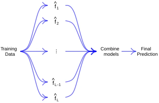
Figure 1 shows a schematic diagram of ensemble learning. For ensemble learning to make sense, we need to inject some sort of variation from one learner to the next, and there many techniques that help us with this task. Among the most common methods to perform ensemble learning are, Bagging (Breiman 1996a), where we perform bootstrapping the observations of the training set, thus selecting a different sample to fit the model, we have random forest (Breiman 2001), which ensembles trees. Random forest tries to find the most important variables to perform the first split (the stump) and thus giving a different
subspace for the models to work on. We also have boosting (Freund 1995); this algorithm also performs bootstrap on the observations but this time giving higher weights to
f ^
L
f ^
L−1
.. . f ^ 2 f ^ 1 Final Prediction Combine models Training Data
Figure 2.1: Ensmble Learning Illustration
ensemble, here the variability comes from selecting different variables to fit the model, this technique will be further discussed in section 2.3. Besides the many different strategies on how to inject variability in each of the models, we need to thing on how to assemble them to make our final prediction. In general, given the set of models F={fˆ1, ...,fˆL} and with
x∗ ∈ X, we can combine all of the prediction in the ensemble as:
ˆ
f(x∗) =
L
X
l=1
αlfˆl(x∗), (2.8)
Where αl is the weight given to the learner fl(.), this weight could be obtained while growing
the ensemble such as in AdaBoosting(Freund and Schapire 1997), or obtained from a separate training set (Zhang and Ma 2012;2015). The way we will be aggregating those models is by taking the prediction of each model and averaging over them, which means
αl = n1, which gives us Equation 2.9 when performing regression:
ˆ
f(x∗) = 1
L
L
X
l=1
ˆ
fl(x∗); (2.9)
When performing logistic regression the final prediction will be most frequent label:
ˆ
f(x∗) = argmax
( L X
l=1
1y= ˆf(l)(x∗)
)
[image:20.612.194.510.103.309.2]It is worth reinforcing the idea that this is not the only way to do this, and there are many other combination schemes (Zhang and Ma 2012;2015). The next question we should be asking is: why is perform ensemble learning instead of using variable selection? Let’s have a closer look at the bias-variance tradeoff. Let Y = f(x) +ε, E(ε) = 0, and Var(ε) =σ2
ε, if we
have a regression ˆf(X), we can use the squared-loss function and find the prediction error of a given point X =x0:
Error(x0) = E[(Y −fˆ(x0))2 |X =x0]
Error(x0) = σ2ε+ (E[ ˆf(x0)]−f(x0))2+ E[ ˆf(x0)−E[ ˆf(x0)]]
Error(x0) = σ2ε+ Bias
2
( ˆf(x0)) + Var( ˆf(x0)) (2.11)
As we can see in Equation 2.11, the error can be partitioned into three parts under the squared loss function. The fist term is the irreducible error and can not be avoided, then we have the squared bias of the estimator off(x0) followed by the variance of ˆf(x0) around the
mean. Ideally, we want to have a low error, hence a low bias and variance, the issue with that is that if we have a very low bias, then our model tends to be more complex and overfits the data, which leads to high variance. On the other hand, if our model is too simple, then the variance is low but the bias is high, and the model is underfitting the data. If we are trying to make a prediction, this is a problem, and this is where ensemble learning becomes useful, because it allows to have many models with low bias (and high variance), but by averaging those low biases model we can bring the variance down as well. Another significant aspect of ensemble is that is that the general error in the ensemble is smaller than the average error of each base learner. The expression that shows this goes as follows (Krogh, Vedelsby, and others 1995); let f(x) be the true function, and let {fˆ1(x), ...,fˆL(x)} be the set of base
learners with averaged prediction ˆfavg(x), and we the error ei( ˆf(x);x) = ( ˆfi(x)−f(x))2, so:
e( ˆfavg(x);x) =
PL
i=1ei( ˆf(x);x)
L −
PL
i=1( ˆfi(x)−fˆavg(x))2
L (2.12)
What Equation 2.12 is telling us, is that the error of the ensemble is the average of the errors of each base learner minus the variance of the ensemble, which means that the more
variability we are able to insert in the ensemble, the smaller the aggregation error will be. Of course, the expected error of aggregation cannot go to zero, as we know we are bounded by the Bayes Risk. This risk which is the infimum risk for all learners, and could only be achieved if we could have the joint distribution PXY, but we can’t reach this risk as we don’t
know the joint distribution. Letf∗(x) =E[Y |X =x], let’s call the risk R(f∗) =R∗, where:
R∗ = inf
f R(f)
Letf :X →Y be any learner, so the risk R(f) is given by:
R(f) = E[E[(f(X)−Y)2 |X]]
R(f) =E[E[(f(X) +E[X |Y] +E[X |Y]−Y)2 |X]]
After some manipulation, we get to:
R(f) = E[(f(X)−E[Y |X])2] +R∗ (2.13)
Therefore, R(f)> R∗, showing that the risk of any technique is at least the Bayes Risk.
Now that we have seen the advantage over aggregating models, let’s have a more detailed look at Random Subspace Method, or also know as Random Subspace Method.
2.3
Random Subspace Method
In Random Subspace Method, we ensemble models by selection different feature subspaces. In this scenario, the features that compose the subspace will be selected uniformly from the feature space. The RSM described in Ho 1998 is shown on algorithm 0.
Algorithm 1 Random Subspace Method
1: Select d≪pto be the size of the subspace;
2: for l=1,...,L do
3: Reform Simple Random Sample without replacement on Feature Space;
4: Fit model ˆfl on the entire training set with the chosen subspace .
5: end for
The final prediction is calculated as shown in equations (2.9) and (2.10).
Y X1 X2 X3 . . . Xi . . . Xp
Obs1 y1 x11 x12 x13 . . . x1i . . . x1p
Obs2 y2 x21 x22 x23 . . . x2i . . . x2p
Obs3 y3 x31 x32 x33 . . . x3i . . . x3p
..
. ... ... ... ... ... ... ... ... Obsj yj xj1 xj2 xj3 . . . xji . . . xjp
..
. ... ... ... ... ... ... ... ... Obsn yn xn1 xn2 xn3 . . . xni . . . xnp
Table 2.1: RSM Visualization
We can also make an adaptive version of this algorithm, so we can not only select variables, but also select observations to compose each model, just as in Bagging, proposed by
Algorithm 2 Adaptive Random Subspace Method
1: Select d≪pto be the size of the subspace;
2: for l=1,...,L do
3: Draw without replacement on Feature Space;
4: Draw with replacement observations from dataset D to create Dl;
5: Fit model ˆfl on selected observations and subspace.
6: end for
Y X1 X2 X3 . . . Xi . . . Xp
Obs1 y1 x11 x12 x13 . . . x1i . . . x1p
Obs2 y2 x21 x22 x23 . . . x2i . . . x2p
Obs3 y3 x31 x32 x33 . . . x3i . . . x3p
..
. ... ... ... ... ... ... ... ... Obsj yj xj1 xj2 xj3 . . . xji . . . xjp
..
. ... ... ... ... ... ... ... ... Obsk yk xk1 xk2 xk3 . . . xki . . . xkp
..
. ... ... ... ... ... ... ... ... Obsn yn xn1 xn2 xn3 . . . xni . . . xnp
Table 2.2: Adaptive Random Subspace Method
Tables 2.1 and 2.2, respectively, illustrate how RSM and Adaptive RSM work. In Table 2.1 the gray columns indicate which variables are selected for a given iteration of the RSM algorithm, and in Table 2.2 shows how the algorithm selects variables, in gray, and
observations, in blue, from the dataset for a given iteration. In the next two sections 2.4 and 3, we will focus on how to select those variables, in other words, we will be giving higher weights to variables that we judge more important with the goal of selecting these variables more often, so we have better models in our ensemble.
2.4
Random Adaptive Subspace Ensemble Learner
Fokoué and Elshrif (2015) proposed Random Adaptive Subspace Ensemble Learner, which is a data-driven way to select the features from the features space. They assigned weights to the feature before beginning the ensemble and choose the subspace based on those weights. One of the ways they propose on how the weight should be computed is by calculating the correlation between the response and each of the predictors when the response is numeric, and the ANOVA F-statistic when the response is a factor. Let’s now see how the RASSEL algorithm works, as described by Fokoué and Elshrif 2015. Algorithm 3 describe the process.
The final prediction for Y given the set of learners F={fˆ1, ...,fˆL} and x∗ ∈ X will be
Algorithm 3 Random Adaptive Subspace Ensemble Learner
1: Select d≪pto be the size of the subspace;
2: for j=1,...,p do 3: if y∈Rn then
4:
rj = corr(xj, y)
5: Create the vectorπ = (π1, ..., πp)T as:
πj =
r2
j
Pp
k=1rk2
. (2.14)
6: end if
7: if y∈ {0,1} then 8:
Fj =
Between groups mean squared by xj
Within group mean squared by xj
9: Create the vectorπ = (π1, ..., πp)T as
πj =
Fj
Pp
k=1Fk
. (2.15)
10: end if
11: end for
0≤πi ≤1 and p
X
j=1
πj = 1
12: for l=1,...,L do
13: for k=1,...,ddo
14: Construct Subspace by drawing{j1, ..., jd} ⊂ {1, .., p} without replacement from
a multinomial:
jk ∼M ultinomial(π1, ..., πp);
15: end for
16: Draw with replacement observations from dataset D to create Dl;
17: Fit ˆfl to Dl in the subspace and observations selected in the previous step.
Chapter 3
Evolutionary Random Adaptive
Subspace Ensemble Learner
In this section, we present the algorithm that is proposed in this thesis. The intuition behind Evolutionary Random Adaptive Subspace Ensemble Learner (ERASSEL) is the same as in RASSEL, select subspaces with data-driven weights, in RASSEL this weights were based on the correlation of the response with the predictors which will lead us to have fixed
throughout the building of the ensemble. With ERASSEL, we will compute those weights based on the l-th model; we will fit the model, calculate the test error for that model and assign it to the subspace that was used to fit that model. Algorithm 4 has more details on how this process works.
3.1
The Algorithm
We will begin by describing how the algorithm works on pseudocode 4, then we will go into more details on how to update the weights described in operation 10 of the algorithm in section 3.2, for regression and section 3.3 for classification.
The idea to do this weighting schemes is two-folded: (a) As we build more models, we will learn which are “good” and “bad” variables; so we can give the “bad” ones smaller
Algorithm 4 Evolutionary Random Adaptive Subspace Ensemble Learner
1: Select d≪pto be the size of the subspace;
2: Initialize weight vector π = (π1, ..., πp) to uniformly select d variables;
3: for l=1,...,L do 4: for k=1,...,ddo
5: Draw {j1, ..., jd} ⊂ {1, .., p} without replacement from multinomial :
jk∼M ultinomial(π1, ..., πp)
6: end for
7: Draw with replacement observations from dataset D to create Dl;
8: Fit model ˆfl on selected observations and subspace;
9: Calculate error made by ˆfl on observationsx6∈Dl;
10: Update variable weights π as function of the error committed by ˆfl
11: end for
3.2
Updating Weights for Regression Tasks
Let’s now describe how the weights are updated in the regression scenario. We will be using the Mean Squared Error (MSE) as a way to assign weights. The MSE for model a ˆf(.) is given by:
MSE = 1
n
n
X
i=1
( ˆf(.)−yi)2
This MSE will be calculated on observations that were not in the training set, in order words, we will be using the m Out Of Bag (OOB) observations to calculated it. We are going to call this the Out Of Bag Error (OOBE), which will be:
OOBE = 1
m
m
X
i=1
I(i∈OOB)( ˆf(xi)−yi)2 (3.1)
So for model ˆfl(.) its OOBE will be stored and assigned to each of the variables that were
part of ˆfl(.), the OOBE for model ˆfl(.) is:
OOBEl =
1
m
m
X
i=1
I(i∈OOB)( ˆfl(xi)−yi)2 (3.2)
In order to update the weights, we want to keep track of all the OOBE’s of a given variable. We want to use that information as a way to give a weight to that variable, so we will create a variable for tracking, which we will call T, and we will do the following updating scheme:
T(l)(Xk) =
( 1
l
Pl−1
i=1T(i)(Xk) + OOBEl
, if Xkwas selected
T(l−1)(X
Finally, we compute the weight for variable Xk for the next iteration:
wkl+1 = exp
n
−T(l)(Xk))
o
Pp
i=1exp{−T(l)(Xk)}
. (3.3)
As for the first round of drawing of variables, we don’t have any OOBE’s yet, so the approach was to assume that every variable might be important, so the all receive
OOBE1 = 0, hence, making all of them have weight equal to one. The advantage of doing
this is that the variables that weren’t selected start having higher weight as we grow the ensemble, that way having a higher probability of showing up in the future models. This agrees with the idea of ensemble learning, because as it was said, we want to insert variability in each learner of the ensemble. Of course, the weights starts to become more stable as the ensemble gets big enough.
3.3
Updating Weights for Classification Tasks
For classification tasks, we will be using the accuracy of the model to compute the weights, which is:
ACC = 1
n
n
X
i=1
1[Y= ˆf(.)]
The accuracy of a model is in the interval [0,1], so the closer to 1 the more accurate is the model. Just as in regression, we will be using the m OOB observations to calculate the accuracy of model ˆf(l)(.), here we will call it the Out Of Bag Accuracy:
OOBA = 1
m
m
X
i=1
I(i∈OOB)I[Y= ˆf(.)] (3.4)
Once more, we want to keep track of the accuracy that was obtained every time a model was fitted, so we will store the accuracy to of each of the variables that participated in the creation of model ˆfl(.). We will again create a variable T to keep track of what is happening
in order to assign the weights, so similarly to Equation 3.3, will have:
T(l)(Xk) =
( 1
l
Pl−1
i=1T(i)(Xk) + OOBAl
, if Xkwas selected
T(l−1)(X
k), Otherwise
And the weight for the next round l+ 1 will simply be:
wlk+1 = T
(l)(X
k)
Pp
i=1T(l)(Xk)
Just as we did in regression, we want to have an optimistic start, so for regression we have the first OOBE a value of zero, here we will set OOBA1 = 1, and again this will give equal
weights to variables in the dataset, and also this will make variables that have not yet been selected as the ensemble grow have higher weights for the next sampling of variables.
With the method on how the weights are updated, we could speculate on what will happen as the size of the ensemble grows. The first thing that comes to mind, is that this scheme will begin to give higher weights to variables that deem themselves important, as said previously. This could be thought of as a kind of variable selection, here might say that this algorithm brings the good aspects of ensemble learning, and also gives the researcher a way of understanding what variables are driving the data. Another thing we could think is, how do the final weights compare to RASSEL; could the weights that are dynamically calculated by ERASSEL converge to the statics weights of RASSEL? Let we(l) and wr be the weights
computed in ERASSEL and RASSEL respectively, and l the ensemble size, perhaps the following could happen:
lim
l→∞w (l)
e =wr
Recall that the importance of ensemble learning is to create variability into each learner and therefore reduce the prediction error by aggregating them. So, if this convergence is in fact happening, we could argue that ERASSEL might be injecting more variability into the beginning of the ensemble, and as the ensemble grows, it begins to build more stable models as in RASSEL. Unfortunately, due to lack of time, this effect will not be theoretically explored in this work but an empirical result will be shown in the Results section.
3.4
Size of Subspace
When performing Random Subspace Learning we have a to choose a smaller number of features than contained in the original dataset, as described in algorithms 0, 2,3 and 4. Breiman (2001) suggested that the size d of the subspace should bed=dp/3e for regression and d=d√pe for classification, but as said in Bryll, Guitierrez-Osuna and Quek (2003) the size of the subspace will change from a problem to another. So, in order to the decide the size of the subspace in the experiments made in section 5, we will first perform ERASSEL with models of size d varying in [0, p] on a sample of 80% from the original dataset, calculate the error on the 20% remaining observation. If there is a size d that yields a clear minimum; otherwise we will use d where elbow of the errors happen. In case there is no clear elbow or clear minimum, we will make use of the recommendation made by Breiman (2001).
3.5
Predictive Performance
R(f) =E[l(Y, f(X))] =
Z
X×Y
l(x, y)dP(x, y). (3.6)
In Equation 3.6 we have a general formulation for risk, let’s define our loss functions for both regression and classification.
3.5.1
Squared Loss
When we perform MLR, the loss function l(Y, f(x)) we want to minimize is the squared loss, which is:
l(Y, f(X)) = (Y −f(X))2 (3.7)
Under the squared loss, we have that the best estimator of f(X) is E[Y |X =x], but this cannot be computed as we don’t have the joint distribution P(y,x), thus to compare the predictive performance of the algorithms we will use the average test error:
AVTE( ˆf) = 1
R R X r=1 ( 1 m m X t=1
l(yi(tr),fˆr(x(irr))) )
(3.8)
Where ˆfr(.) is the r-th model build with the data (x(r), y(r)). Namely, the average test error
shown in (3.8) will be the mean squared error (MSE):
MSE( ˆf) = 1
n
n
X
i=1
(yi−fˆ(xi))2 (3.9)
It is important to notice how this function is sensitive to large distances, as we are squaring those high values, we could be using the L1 as in LASSO regression (Tibshirani 1996) function which uses the module instead of the squared function. We will now look at the Zero-One loss function.
3.5.2
Zero-One Loss
For the classification tasks, we will use the zero-one loss, which is defined as:
l(Y, f(X)) = 1[Y6=f(x)] (3.10)
The average test error here will be the classification error rate which will be:
AVTE( ˆf) = 1
n
n
X
i=1
Chapter 4
Data
As a way to compare all the algorithms we have described, we will test them in different situations. First, we will be using simulated data in two distinct scenarios, one with
orthogonal data and another data that has multicollinearity; then we will use real word data. Both, simulated and real world data, will be described below.
4.1
Simulated Data
In order to compare the algorithm, they will be first tested by using simulated data that way we have more control over what is happening in the data. We will simulate data for that is suitable to perform regression and data for logistic regression.
4.1.1
Simulated Data for Multiple Linear Regression
We will simulate the data to perform regression analysis as following:
X ∼Np(µ,Σ)
,
where µ∈Rp and Σ a p×ppositive semi-definite matrix. We have that the Multivariate
Normal is denoted by:
φ(x;µ,Σ) = q 1
(2π)p |Σ|exp
1
2(x−µ)
TΣ−1
(x−µ)
. (4.1)
For this simulation we will have that the true, but unknown, function that is generating the response is given by:
,
with ε ∼N(0,4). We will create three hundred observation and ten variables using this method.
4.1.2
Simulated Data for Logistic Regression
In a similar way as described in section 4.1.1, we will use 4.1 to generate the variable. The difference is that now we will need to have a dictonomic response Y. To achieve this, we will begin by creating Y as a function of X1,X4 and X5:
η(X) = 1 +X1 +X4+X5,
Now, we will use the logit transformation on the response:
πi =
1
1 + exp{−η(xi;β)}
This will return values for πi in the interval [0,1]. Finally, in order to have the binary
response we will simply do the following then in order to assign a class toY we will sample from a Bernoulli:
Yi ∼Bern(πi)
Just as in the simulation for regression, we will be simulating 300 observations with 10 variables.
4.1.3
Real Data
Besides the simulated data, we also want to see how the algorithms perform with real data. We will use data that is available on statistical software R (R Core Team 2015) and libraries MASS (Venables and Ripley 2002), mlbench (Leisch and Dimitriadou 2010), kernlab
(Karatzoglou et al. 2004) and ggplot2(Wickham 2009). We will also make use of the prostate cancer dataset (Stamey et al. 1989), which has a situation where p≫n, which means that we would have a lot of trouble fitting a regular linear model here, and thus RSSL becomes very useful in this situation. Table 4.1 has more information on the datasets that we will be used, such as dimension, the task that will be performed and the response variable1 of each
dataset.
Dataset Observations Variables Response Task
Boston 506 14 Per capita crime rate1 Regression
Diamonds 53940 7 Weight of diamond Regression
Cars932 93 16 Car Price1 Regression
Spam 4601 58 E-mail is spam or not spam Classification
Pima 532 8 Pima Indian women with diabetes or not Classification
Ionosphere 531 35 Good or bad structure in the ionosphere Classification
Prostate 79 501 Patient has prostate cancer or not Classification
Table 4.1: Data Sets
4.2
Implementation
Chapter 5
Experiments and Results
The comparative results for the simulated data will be presented in this section, both in regression and logistic regression. Firstly, we will show the results from the simulated data, along with other features of the algorithm. Then we will show all four algorithms described in sections 2.3, 2.4 and 3 compare to each other. For each of the comparisons, we will split the dataset into training and test sets, where 70% of the data will be used to as the training set, when performing classification we want both classes to appear to on both training and test sets, so we will perform a stratified sample on both labels with 70% each label on the training set and 30% on the test set. When the splitting of the data is done, we will fit the models by using each of the algorithms to the training set and calculate the error on the test. The process of splitting the data, fitting models and calculating the errors will be replicated fifty times. Each of the ensemble will be composed of two hundred models, besides that, as described in algorithm 4, ERASSEL computes the out of bag error, so the training set will again be split into two where 30% will be used in order to calculate the out of bag error.
5.1
ERASSEL at Work
Before comparing the algorithm, let’s we take this opportunity to show how the algorithm for ERASSEL is working under the hood. To achieve that, we will begin by showing how the weight changes over time and the final weights given to every variable in the feature space; we will also show how it performs when there are highly correlated variables in the dataset.
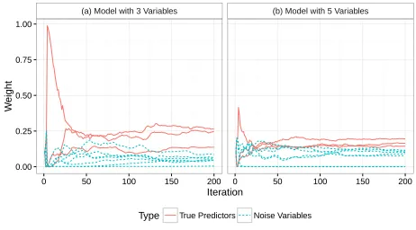
First, let’s see how ERASSEL performs with the simulated data and if the algorithm is able to pick the actual variables that are generating the process. So, for this simulated problem, we will run two scenarios, one where the number of variables in the models in the ensemble is exactly the number of variables of the true function, and another one where we will set the number of variables to a larger number, for this example, we will use five variables. This means that we should see ERASSEL assign higher weights to X1, X4 and X5 than the
(a) Model with 3 Variables (b) Model with 5 Variables
0.00 0.25 0.50 0.75 1.00
0 50 100 150 200 0 50 100 150 200
Iteration
W
eight
Type True Predictors Noise Variables
Figure 5.1: Variable Weight Path - Orthogonal Data
(a) Model with 3 Variables (b) Model with 5 Variables
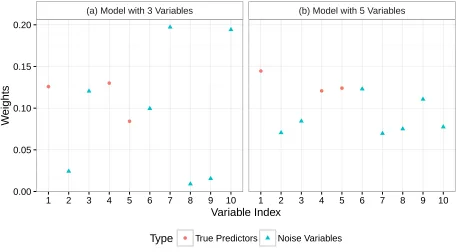
0.0 0.1 0.2
1 2 3 4 5 6 7 8 9 10 1 2 3 4 5 6 7 8 9 10
Variable Index
W
eights
Type True Predictors Noise Variables
[image:35.612.75.537.88.344.2] [image:35.612.79.538.418.671.2]As we can see, Figure 3 shows that in both cases, with three and five variables, X1, X4 and X5 were given the three highest weights. As mentioned in section 2.4, RASSEL assign a
priori weights to each feature, here in this weight based on the features correlation with the response variables. Let’s see how the fixed weights from RASSEL compare to ERASSEL’s dynamic approach.
0.0 0.1 0.2 0.3 0.4
1 2 3 4 5 6 7 8 9 10
Variable
W
eights
Method ERASSEL RASSEL
Figure 5.3: Final Variable Weight - Final Weights Comparison between ERASSEL and RASSEL
Figure 4 shows that for this simulation, these weights have the same pattern, with the important variables X1, X4 and X5 having the highest weights, in fact, they are even in the
same order relative to one another, i.e., in both algorithm X4 was assigned the highest
weights, followed by X5 then X1.
We have seen that ERASSEL can pick up the variables that are generating the response. Let’s see what happens when we have highly correlated data. In order to this, we will make
X7 a linear function of X1 and introduce some noise. This is the linear function we will use:
X7 = 2X1+η
where η∼N(0,1). Letρˆbe the correlation matrix of the simulated data obtained after performing this transformation on X7. As we can see the correlation between X1 and X7 is
[image:36.612.84.538.160.414.2]ˆ ρ=
1.00 0.45 −0.32 0.19 −0.35 −0.03 0.87 0.33 0.38 −0.09 0.45 1.00 0.29 −0.04 −0.06 −0.40 0.30 0.41 0.44 0.44
−0.32 0.29 1.00 0.30 −0.42 −0.38 −0.29 0.15 0.34 0.30
0.19 −0.04 0.30 1.00 −0.54 −0.06 0.35 −0.08 0.05 −0.50
−0.35 −0.06 −0.42 −0.54 1.00 −0.26 −0.34 0.02 −0.69 −0.17
−0.03 −0.40 −0.38 −0.06 −0.26 1.00 0.13 −0.38 0.25 0.05
0.87 0.30 −0.29 0.35 −0.34 0.13 1.00 0.13 0.41 −0.14 0.33 0.41 0.15 −0.08 0.02 −0.38 0.13 1.00 0.29 0.02 0.38 0.44 0.34 0.05 −0.69 0.25 0.41 0.29 1.00 0.67
−0.09 0.44 0.30 −0.50 −0.17 0.05 −0.14 0.02 0.67 1.00
Let’s see how this will affect ERASSEL.
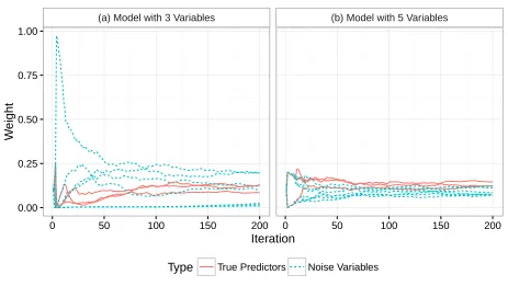
(a) Model with 3 Variables (b) Model with 5 Variables
0.00 0.25 0.50 0.75 1.00
0 50 100 150 200 0 50 100 150 200
Iteration
W
eight
Type True Predictors Noise Variables
Figure 5.4: Variable Weight Path - With Multicolinearity
[image:37.612.76.539.281.542.2](a) Model with 3 Variables (b) Model with 5 Variables
0.00 0.05 0.10 0.15 0.20
1 2 3 4 5 6 7 8 9 10 1 2 3 4 5 6 7 8 9 10
Variable Index
W
eights
Type True Predictors Noise Variables
Figure 5.5: Variable Weights - With Multicolinearity
5.2
Comparative Results
Now that we have seen how ERASEEL works, we will compare how the four algorithms described previously compare with one another. As mentioned before, we will compare their respective errors, and see which of the algorithms yields the best results.
5.3
Regression
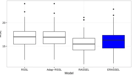
Let’s begin by comparing how they perform when aggregating regression models. We will begin by the simulated data with no correlation between variables, then we will move on to real data. We will begin by choosing the size of the subspace then proceed to fitting the models and calculating their errors, these last two steps will be done 50 times as mentioned before. Also as a reminder, the original dataset will be split into training, with 70% of the data and test containing the remaining 30%.
As defined in section 3.4, we will select the size of the subspace as the size that yields the smallest MSE by fitting RASSEL to sample of the training data. In Figure 7 we see that the error decreases until we reach 5 variables in the subspace, then it begins to increase again, so we will select 5 as the size for our models.
[image:38.612.79.536.76.328.2]13.5 14.0 14.5
1 2 3 4 5 6 7 8 9 10
Model Size
MSE
Figure 5.6: Best Model Size - Simulated Regression
15 20
RSSL Adap−RSSL RASSEL ERASSEL
Model
MSE
[image:39.612.80.535.89.344.2] [image:39.612.84.537.418.677.2]Model Mean Median Var
1 RSSL 17.00 16.99 5.73
2 Adap-RSSL 16.98 16.94 5.59
3 RASSEL 15.52 15.47 4.86
4 ERASSEL 16.17 16.30 6.11
Table 5.1: MSE Summary by Model - Simulated Regression Data
0.6 0.8 1.0 1.2
1 2 3 4 5 6 7 8 9 10 11 12 13
Model Size
MSE
Figure 5.8: Best Model Size - Boston Dataset
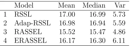
Figure 9 shows that it very hard to pick the size of the subspace, as every variable we add the prediction improves, but let’s pick 7 as the number of variable for our models, since it is a little over half of the total number of variable in the dataset.
Looking at 5.2 and Figure 10 we see that just as with the simulated data, the best ensemble algorithm is RASSEL, followed by ERASSEL. It is interesting to see that they all minuscule variance.
[image:40.612.200.414.70.146.2] [image:40.612.82.538.192.451.2]Model Mean Median Var
1 RSSL 0.69 0.69 0.01
2 Adap-RSSL 0.69 0.69 0.01
3 RASSEL 0.64 0.64 0.01
4 ERASSEL 0.67 0.67 0.01
Table 5.2: MSE Summary by Model - Boston Dataset
0.5 0.6 0.7 0.8 0.9
RSSL Adap−RSSL RASSEL ERASSEL
Model
MSE
Figure 5.9: Boxplot of Errors by Model - Boston Dataset
[image:41.612.80.537.183.444.2]0.01 0.02 0.03 0.04
1 2 3 4 5 6
Model Size
MSE
Figure 5.10: Best Model Size - Diamond Dataset
5 10 15 20
RSSL Adap−RSSL RASSEL ERASSEL
Model
MSE (x 1000)
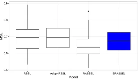
[image:42.612.79.536.89.343.2] [image:42.612.81.537.417.675.2]Model Mean Median Var
1 RSSL 8.88 7.92 7.69
2 Adap-RSSL 8.76 7.48 8.51
3 RASSEL 8.13 6.53 16.45
4 ERASSEL 8.74 7.57 8.42
Table 5.3: MSE( x 1000) Summary by Model - Diamonds Dataset
0.08 0.10 0.12 0.14
1 2 3 4 5 6 7 8 9 10 11 12 13 14 15
Model Size
MSE
Figure 5.12: Best Model Size - Car93 Dataset
Based on Figure 13 we picked seven as the number of variables in the model.
We can see that for this dataset RASSEL didn’t perform as well as before, in fact plain RSSL was the best algorithm. With this we have finished the experiments for regression, as we saw, mostly RASSEL performed slightly better than the others, but the differences in the results aren’t that significant as we can see the means are very close to each other;
[image:43.612.83.535.195.448.2]Model Mean Median Var
1 RSSL 57.29 57.16 344.15
2 Adap-RSSL 57.60 57.50 357.73
3 RASSEL 58.47 56.71 349.55
4 ERASSEL 57.79 59.17 347.89
Table 5.4: MSE( x 1000) Summary by Model - Cars93 Dataset
25 50 75 100 125
RSSL Adap−RSSL RASSEL ERASSEL
Model
MSE (x 1000)
Figure 5.13: Boxplot of Errors by Model - Boston Dataset
5.4
Classification
Now, let’s see how those algorithms compare when performing classification tasks. Just as we did for regression, let’s begin by looking at the results for the simulated data and then real data. We will also follow the same steps as we did for regression - choose the size of subspace, fit models and calculate the error.
It seems that after models of size seven the error stabilizes and does not decrease that much. So let’s use seven as the size of our models for this problem.
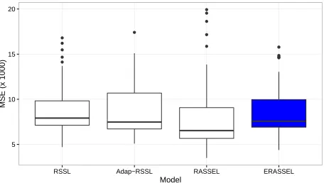
By looking at Figure 16 and Table 5.5 we can see that RSSL and RASSEL are performing better than the other two ensemble methods on the predicting the simulated data. Next, we can see how the methods compare with the real world data.
Based on Figure 17 it seems that 33 will be a good model size for the spam dataset.
The Spam dataset was exhaustively analyzed in Fokoué and Ly (2014), they found,
[image:44.612.79.536.183.445.2]0.2 0.3 0.4 0.5 0.6
1 2 3 4 5 6 7 8 9 10
Model Size
Error Rate
Figure 5.14: Best Model Size - Simulated Logistic Regression
15 20 25 30
RSSL Adap−RSSL RASSEL ERASSEL
model
Error
[image:45.612.79.537.88.346.2] [image:45.612.84.537.418.677.2]0.10 0.15 0.20 0.25
1 2 3 4 5 6 7 8 9 10 11 12 13 14 15 16 17 18 19 20 21 22 23 24 25 26 27 28 29 30 31 32 33 34 35 36 37 38 39 40 41 42 43 44 45 46 47 48 49 50 51 52 53 54 55 56 57
Model Size
Error Rate
Figure 5.16: Best Model Size - Spam Dataset
6 7 8 9
RSSL Adap−RSSL RASSEL ERASSEL
model
Error
[image:46.612.80.536.88.344.2] [image:46.612.84.537.418.676.2]Model Mean Median Var
1 RSSL 20.82 20.62 11.38
2 Adap-RSSL 21.29 21.01 11.90
3 RASSEL 21.29 21.01 11.90
4 ERASSEL 21.04 21.01 11.93
Table 5.5: Error Rate Summary by Model - Simulated Logistic Regression
Model Mean Median Var
1 RSSL 7.56 7.60 0.44
2 Adap-RSSL 7.42 7.46 0.36
3 RASSEL 7.42 7.46 0.36
4 ERASSEL 7.38 7.46 0.44
Table 5.6: Error Rate Summary by Model - Spam Data
3.6% error rate by using Ensembled Decision Trees. Here we have that ERASSEL had the smallest error rate out of the four methods compared, at 7.38%, RSSL was the one that had the worst median, the results are found in Table 5.6 and Figure 18.
Looking at Figure 19 we see that the minimum error occurs when we have seven variables in the model. Obviously, it wouldn’t make sense to use RSM if we used every variable in the dataset, so the next best value to select as the model size seems to be three variables, where it stabilizes.
Model Mean Median Var
1 RSSL 22.48 22.36 5.21
2 Adap-RSSL 22.65 22.98 5.31
3 RASSEL 22.65 22.98 5.31
4 ERASSEL 22.67 22.36 5.72
Table 5.7: Error Rate Summary by Model - Pima Data
0.24 0.26 0.28 0.30
1 2 3 4 5 6 7
Model Size
Error Rate
Figure 5.18: Best Model Size - Pima Dataset
20 25
RSSL Adap−RSSL RASSEL ERASSEL
model
Error
[image:48.612.80.535.89.343.2] [image:48.612.83.537.417.674.2]0.2 0.4 0.6
1 2 3 4 5 6 7 8 9 10 11 12 13 14 15 16 17 18 19 20 21 22 23 24 25 26 27 28 29 30 31 32 33
Model Size
Error Rate
Figure 5.20: Best Model Size - Ionosphere Dataset
Looking at Figure 21 it seems that after eleven variables in the model, there isn’t much change in the error.
Model Mean Median Var
1 RSSL 11.42 11.79 7.24
2 Adap-RSSL 11.06 10.38 6.83
3 RASSEL 11.06 10.38 6.83
4 ERASSEL 10.83 10.85 6.29
Table 5.8: Error Rate Summary by Model - Ionosphere Data
[image:49.612.79.538.74.336.2]10 15 20
RSSL Adap−RSSL RASSEL ERASSEL
model
Error
Figure 5.21: Boxplot of Errors by Model - Ionosphere Dataset
0.2 0.3 0.4 0.5 0.6
RSSL Adap−RSSL RASSEL ERASSEL
model
Error
[image:50.612.85.537.88.348.2] [image:50.612.86.537.418.676.2]Model Mean Median Var
1 RSSL 0.38 0.36 0.01
2 Adap-RSSL 0.39 0.40 0.01
3 RASSEL 0.39 0.40 0.01
4 ERASSEL 0.36 0.36 0.01
Table 5.9: Error Rate Summary by Model - Prostate Data
As we can see, ERASSEL seems to be doing a good job on this dataset; it has the smaller median and smaller variation than all other algorithms, plain RSSL also seems to be doing well. Adap-RSSL and RASSEL are doing performed extremely similar. This dataset
Chapter 6
Conclusion and Future Work
In this thesis, we have presented a new algorithm for ensemble learning, which is a common technique in Machine Learning, specially for when the task is mainly to make predictions. The focus of this new algorithm was Random Subspace learning, which focuses on selecting different subspaces of the feature space, and thus creating variation in the base learners. Random subspace learning is an important method for ensemble learning, as it allows for fitting model on conditions that might not be ideally for fitting common statistical models, namely when n≫p. This algorithm focuses assigning weights to variables in the feature space. The interesting aspect of different weighting schemes for random subspace learning is that important not to waste computing time by looking at variables that are not useful to predict our response.
The way this algorithm works is that as the ensemble grows, it update the variables weights based previous models of the ensemble to select the next subspace, that way giving more weight to variables that prove to be important in predicting the response and avoiding using variables that do not help on the prediction. This idea came from the much known evolution of species in the natural world, where good features survive throughout the environment and bad traits tend to die off, or least be less common. with that in mind, the algorithm was called Evolutionary Adaptive Random Subspace Learning.
We have shown that ERASSEL can be used for regression and classification tasks, the only adjustment needed is on how the updating of weight works, which have been presented in this work. The base learners used in order to perform the empirical test was GLM, which is widely applied in the statistical community and can be easily adapted to different situations, such as regression and classification. It is important to keep in mind that ERASSEL could be adapted to many other learners, such as classification and regression trees or SVM.
After looking how behind the curtains, we used simulated and real data for both regression and classification to compare it with plain RSSL, Adaptive RSSL, and RASSEL, which showed us that ERASSEl is comparable to algorithms already well established in the data mining community. Although, it was shown that RASSEL performs better than ERASSEL and the others for regression tasks. As for classification, ERASSEL was more comparable to RASSEL, and it perform very well on the dataset where we had more variables than
observations.
Appendix A
Selected R Code
################################################################################
# PACKAGES #
################################################################################ library(mlbench)
library(kernlab) library(datasets) library(sampling) library(MASS) library(ggplot2) library(reshape2) library(dplyr)
################################################################################
# FUNCTIONS #
# For Random Subspace Learning #
################################################################################
################################################################################ ############################### Regression ##################################### ################################################################################
##### RSSL #########
rssl.lm<-function(response,data,d,L){ n<-nrow(data)
p<-ncol(data)
for( i in 1:L){
sel.sub<-sample(c(1:p)[-resp.pos],d,replace = F) subs.data<-paste(names(data)[sel.sub],collapse = "+") form<-as.formula(paste0(response,"~",subs.data)) m<-lm(form,data)
mod.list<-c(mod.list,list(m)) }
return(mod.list) }
#### Adaptive RSSL uniform weight ####
rsslbag.lm<-function(response,data,d,L,size){ n<-nrow(data)
p<-ncol(data)
resp.pos<-which(names(data)==response) mod.list<-NULL
for( i in 1:L){
sel.obs<-sample(1:n,size,replace=T)
sel.sub<-sample(c(1:p)[-resp.pos],d,replace = F) subs.data<-paste(names(data)[sel.sub],collapse = "+") form<-as.formula(paste0(response,"~",subs.data)) m<-lm(form,data[sel.obs,])
mod.list<-c(mod.list,list(m)) }
return(mod.list) }
#### Adaptive RASSEL ####
rassel.lm<-function(response,data,d,L,size){ n<-nrow(data)
p<-ncol(data)
resp.pos<-which(names(data)==response) cor.resp<-cor(data)[,response][-resp.pos] weight.sel<-cor.resp^2/sum(cor.resp^2) mod.list<-NULL
for( i in 1:L){
sel.sub<-sample(c(1:p)[-resp.pos],d,replace = F,prob=weight.sel) subs.data<-paste(names(data)[sel.sub],collapse = "+")
form<-as.formula(paste0(response,"~",subs.data)) m<-lm(form,data[sel.obs,])
mod.list<-c(mod.list,list(m)) }
return(mod.list) }
####### Evolutionary RASSEL ########
erassel.lm<-function(response,da