Testing equality of two intercepts for the parallel regression model with non-sample prior information

Regression Model with Non-sample Prior Information

Budi Pratikno1 _{and Shahjahan Khan}2 1 _{Department of Mathematics and Natural Science}

Jenderal Soedirman University, Purwokerto, Jawa Tengah, Indonesia 2 _{School of Agricultural, Computational and Environmental Sciences}

Centre for Sustainable Catchments, University of Southern Queensland Toowoomba, Queensland, Australia

Email: b [email protected] and [email protected]

Abstract

This paper proposes tests for equality of intercepts of two simple regression models when non-sample prior information (NSPI) is available on the equality of two slopes. For three different scenarios on the values of the slope, namely (i) unknown (unspecified), (ii) known (specified), and (iii) suspected, we derive the unrestricted test (UT), restricted test (RT) and pre-test test (PTT) for testing equality of intercepts. The test statistics, their sampling distributions, and power functions of the tests are obtained. Comparison of power function and size of the tests reveal that the PTT has a reasonable dominance over the UT and RT.

Keywords and phrases: Linear regression; intercept and slope parameters; pre-test pre-test; non-sample prior information; and power function.

2010 Mathematics Subject Classification: Primary 62F03 and Secondary 62J05.

1

Introduction

Inferences about population parameters could be improved using non-sample prior information (NSPI) from trusted sources (cf Bancroft, 1944). Such information are usually available from previous studies or expert knowledge or experience of the researchers, and are unrelated to any sample data.

It is well known that, for any linear regression model, the inference on the intercept parameter depends on the value of the slope param-eter. Thus the non-sample prior information on the value of the slope parameter would directly affect the inference on the intercept parameter.

An appropriate statistical test on the suspected value of the slopes, after express-ing it in the form a null hypothesis, is useful to eliminate the uncertainty on this suspected information. Then the outcome of the preliminary test on the uncertain NSPI on the slopes is used in the hypothesis testing on the intercepts to improve the performance of the statistical test (cf. Khan and Saleh, 2001; Saleh, 2006, p. 55-58; Yunus and Khan, 2011a).

As an example, in any spotlight analysis the aim is to compare the mean re-sponses of the two categorical groups at specific values of the continuous covariate. Furthermore, we consider a response variable (η), a continuous covariate (χ) and a categorical explanatory variable (ζ) with two categories (eg treatment and control). If there is an association between χ and ζ, the least squares line of η on χ will be parallel with different intercepts for two different categories ofζ. However, the two fitted lines will not be parallel if there is no association between the two explanatory variables because of the presence of interaction. The scenario will be different if the two explanatory variables are associated and they also interact.

In any inference, estimation or test, on the equality of the two intercepts of the two regression lines of Y on X for two different categories of Z, the slope of the regression lines plays a key role. The test (also the estimation) of intercept is directly impacted by the values of the slope. Therefore, the type of NSPI on the value of the slopes will influence the inference on the intercepts.

The suspected NSPI on the slopes may be (i) unknown or unspecified if NSPI is not available, (ii) known or specified if the exact value is available from NSPI, and (iii) uncertain if the suspected value is unsure. For the three different scenarios, three different statistical tests, namely the (i) unrestricted test (UT), (ii) restricted test (RT) and (iii) pre-test test (PTT) are defined.

In the area of estimation with NSPI there has been a lot of work, notably Ban-croft (1944, 1964), Hand and BanBan-croft (1968), and Judge and Bock (1978) intro-duced a preliminary test estimation of parameters to estimate the parameters of a model with uncertain prior information. Khan (2000, 2003, 2005, 2008), Khan and Saleh (1997, 2001, 2005, 2008), Khan et al. (2002), Khan and Hoque (2003), Saleh (2006) and Yunus (2010) covered various work in the area of improved esti-mation using NSPI, but there is a very limited number of studies on the testing of parameters in the presence of uncertain NSPI. Although Tamura (1965), Saleh and Sen (1978, 1982), Yunus and Khan (2007, 2011a, 2011b), and Yunus (2010) used the NSPI for testing hypotheses using nonparametric methods, the problem has not been addressed in the parametric context.

equations, namely

y1j =θ1+β1x1j+e1j and y2j =θ2+β2x2j+e2j, j=1,2,· · · ,ni,

for the two data sets: y = [y′₁,y₂′]′ and x = [x′₁,x′₂]′ where y₁ = [y11,· · · , y1n1]

′

,

y₂ = [y21,· · ·, y2n2]

′

, x1 = [x11,· · · , x1n1]

′

and x2 = [x21,· · · , x2n2]

′

, we use an appropriate two-samplettest for testingH0:β1=β2 (parallelism). Thiststatistic is given as

t= βe1−βe2

S_(fβ

1−fβ2)

,

where βe1 and βe2 are estimate of the slopes β1 and β2 respectively, andS_(βf

1−fβ2) is

the standard error of the estimated difference between the two slopes (Kleinbaum et al., 2008, p. 223). The parallelism of the two regression equations above can be expressed as a single model in matrix form, that is,

y=XΦ+e,

where Φ = [θ1, θ2, β1, β2]

′

, X = [X1,X2]

′

with X1 = [1,0, x1,0]

′

and X2 = [0,1,0, x2]

′

ande= [e1, e2]

′

. The matrix form of the intercept and slope parameters can be written, respectively, asθ = [θ1, θ2]

′

and β= [β1, β2]

′

(cf Khan, 2006). For the model under study two independent bivariate samples are considered such that yij ∼ N(θi+βixij, σ2) for i = 1,2 and j = 1,· · · , ni. See Khan (2003, 2006, 2008) for details on parallel regression models and related analyses.

To explain the importance of testing the equality of the intercepts when the equality of slopes is uncertain, we consider the general form of the two parallel simple regression models (PRM) as follows

Yi =θi1ni+βixij+eij, i= 1,2, and j=1,2,· · · ,ni, (1.1)

where Yi = (Yi1,· · ·, Yini) ′

is a vector of ni observable random variables, 1ni = (1,· · ·,1)′ is an ni-tuple of 1′s, xij = (xi1,· · · , xini)′ is a vector of ni indepen-dent variables, θi and βi are unknown intercept and slope, respectively, and ei = (ei1,· · · , eini)′ is the vector of errors which are mutually independent and identically distributed as normal variable, that is, ei ∼ N(0, σ2Ini) where Ini is the identity matrix of orderni. Equation (1.1) represents two linear models with different inter-cept and slope parameters. Ifβ1 =β2 =β, then there are two parallel simple linear models when θ_i′s are different.

the power is preferred over any other tests. In reality, the size of a test is fixed, and then the choice of the best test is based on its maximum power.

This study considers testing the equality of the two intercepts when the equality of slopes is suspected. For which we focus on three different scenarios on the slope parameters, and define three different tests:

(i) for the UT, letϕU T be the test function andTU T be the test statistic for testing

H0 :θ=θ0 againstHa:θ>θ0 when β= (β1, , β2)

′

is unspecified,

(ii) for the RT, letϕRT be the test function andTRT is the test statistic for testing

H0 :θ=θ0 againstHa:θ>θ0 when β=β012 (fixed vector),

(iii) for the PTT, let ϕP T T be the test function and TP T T be the test statistic for testing H0 : θ = θ0 against Ha : θ > θ0 following a pre-test (PT) on the slope parameters. For the PT, let ϕP T be the test function for testing

H₀∗ :β = β01p (a suspected constant) against Ha∗ : β > β012 to remove the uncertainty. If theH₀∗ is rejected in the PT, then the UT is used to test the intercept, otherwise the RT is used to testH0. Thus, the PTT onH0 depends on the PT onH₀∗, and is a choice between the UT and RT.

The unrestricted maximum likelihood estimator or least square estimator of intercept and slope vectors,θ= (θ1, θ2)

′

and β= (β1, β2)

′

, are given as

e

θ =Y −Tβe and βe = (x

′

iyi)−(n1i)[1

′

ixi1

′

iyi] niQi

, (1.2)

whereθe= (θe1,θe2)

′

, βe = (βe1,βe2)

′

,T = Diag(x1,x2),niQi =x ′

ixi−(_ni1) [

1′_ixi ]

and

e

θi =Yi−βeixi fori= 1,2.

Furthermore, the likelihood ratio (LR) test statistic for testing H0 : θ = θ0 againstHa:θ>θ0 is given by

F = θe

′

H′D−₂₂1Hθe

s2 e

, (1.3)

where H = I2 − _nQ1 121

′

2D−221, D−221 = Diag(n1Q1,· · ·,n2Q2), nQ =

∑2

i=1niQi,

niQi=x ′

ixi−_ni1(1 ′

ixi)2 ands2e = (n−4)−1 ∑p

i=1(Y−θei1ni−βxe i) ′

(Y −θei1ni−βxe i) (Saleh, 2006, p. 14-15). UnderH0,F follows a centralF distribution with (1, n−4) degrees of freedom, and underHait follows a noncentralFdistribution with (1, n−4) degrees of freedom and noncentrality parameter∆2/2, where

∆2 = θ

′

H′D−₂₂1Hθ

σ2 =

(θ−θ0)′H′D₂₂−1H(θ−θ0)

σ2

= (θ−θ0)

′

D22(θ−θ0)

and D22 = H

′

D−₂₂1H. When the slopes (β) are equal to β012 (specified), the restricted maximum likelihood estimator of the intercept and slope vectors are given as

b

θ=θe+T Hβe and βb = 1k1

′ kD−

1 22βe

nQ . (1.5)

Section 2 provides the proposed three tests. Section 3 derives the distribution of the test statistics. The power function of the tests are obtained in Section 4. An illustrative example is given in Section 5. The comparison of the power of the tests and concluding remarks are provided in Sections 6 and 7.

2

The Proposed Tests

To test the equality of two intercepts when the equality of the slopes is suspected, we define three different test statistics as follows.

(i) For unspecified β , the test statistic of the UT for testing H0 :θ =θ0 against

Ha: θ>θ0, under H0, is given by

TU T = θe

′

H′D−₂₂1Hθe

s2_ut , (2.1)

where

s2_ut= (n−4)−1 2

∑

i=1

(Y −θei1ni−βxe i) ′

(Y −θei1ni−βxe i).

The TU T follows a central F distribution with (1, n−4) degrees of freedom (d.f.). UnderHa, it follows a noncentralF distribution with (1, n−4) d.f. and noncentrality parameter ∆2/2. Under the normal model we have

( e θ−θ e β−β

)

∼N4

[ (

0 0

)

, σ2

(

D11 −T D22

−T D22 D22

) ]

, (2.2)

whereD11=N−1+T D22T β and N= Diag(n1,· · · ,n2).

(ii) Forspecifiedvalue of the slopes,β=β012 (fixed value), the test statistic of the RT for testingH0 :θ=θ0 againstHa:θ>θ0 underH0, is given by

TRT = (bθ

′

H′D−₂₂1Hbθ) + (βe ′

H′D−₂₂1Hβe)

s2 rt

where

s2_rt= (n−2)−1 2

∑

i=1

(Y −θbi1ni−βxb i) ′

(Y −θbi1ni−βxb i) and βb =β012.

The TRT _{follows a central F distribution with (1, n −4) d.f.. Under H} a, it follows a noncentral F distribution with (1, n−4) d.f. and noncentrality parameter∆2/2. Again, note that

( b θ−θ b β−β

)

∼N4

[ ( T Hβ

0

)

, σ2

(

D∗₁₁ D∗₁₂ D∗₁₂ D22

) ]

, (2.4)

whereD∗₁₁=N−1+T121

′

2T β

nQ and D∗12=−nQ1 121 ′

2T.

(iii) When the value of the slope issuspectedto be β=β012 but unsure, a pre-test on the slope is required before testing the intercept. For the preliminary test (PT) ofH₀∗ :β=β01p againstHa∗:β> β012, the test statistic under the null hypothesis is defined as

TP T = βe

′

H′D−₂₂1Hβe

s2_ut , (2.5)

which follows a centralF distribution with (1, n−4) d.f.. UnderHa, it follows a noncentral F distribution with (1, n−4) d.f. and noncentrality parameter ∆2/2. Again, note that

( e

θ−β012

e β−βb

)

∼N4

[ (

(βf∗−β0)12

Hβ )

, σ2

(

121

′

2/nQ 0

0 HD22

) ]

,(2.6)

wherefβ∗12= 121

′

2D

−1

22β

nQ (cf. Saleh, 2006, p. 273).

Let us choose a positive number αj (0< αj < 1,for j = 1,2,3) and real value

Fν1,ν2,αj (with ν1 as the numerator d.f. andν2 as the denominator d.f.) such that

P(TU T > F1,n−4,α1 |θ =θ0

)

= α1, (2.7)

P(TRT > F1,n−4,α2 |θ =θ0

)

= α2, (2.8)

P(TP T > F1,n−4,α3 |β=β012

)

= α3. (2.9)

Now the test function for testingH0:θ =θ0 against Ha:θ >θ0 is defined by

Φ =

{

1, if(TPT ≤Fc,TRT>Fb

)

or(TPT>Fc,TUT>Fa

)

;

0, otherwise, (2.10)

3

Sampling Distribution of Test Statistics

To derive the power function of the UT, RT and PTT, the sampling distribution of the test statistics proposed in Section 2 are required. For the power function of the PTT the joint distribution of (TU T, TP T) and (TRT, TP T) is essential. Let{Nn}be a sequence of local alternative hypotheses defined as

Nn: (θ−θ0,β−β012) =

( λ1

√

n,

λ2

√

n

)

=λ, (3.1)

where λ is a vector of fixed real numbers and θ is the true value of the intercept. The local alternative is used only to compute the power of the tests for specific values of the parameters. UnderNn the value of (θ−θ0) is greater than zero and underH0 the value of (θ−θ0) is equal zero.

Following Yunus and Khan (2011b) and equation (2.1), we define the test statistic of the UT whenβ is unspecified, underNn, as

T₁U T = TU T −n

{

(θ−θ0)

′

H′D−₂₂1H(θ−θ0)

s2_ut

}

. (3.2)

TheT₁U T follows a noncentralF distribution with noncentrality parameter which is a function of (θ−θ0) and (1, n−4) d.f., under Nn.

From equation (2.3) underNn, (θ−θ0)>0 and (β−β012)>0, the test statistic of the RT becomes

T₂RT =TRT−n

{

(θ−θ0)

′

H′D−₂₂1H(θ−θ0) + (β−β012)

′

H′D−₂₂1H(β−β012)

s2_rt

}

.

(3.3) The T₂RT also follows a noncentral F distribution with a noncentrality parameter which is a function of (θ−θ0) and (1, n−4) d.f., under Nn. Similarly, from the equation (2.5) the test statistic of the PT is given by

T₃P T =TP T −n

{

(β−β012)

′

H′D−₂₂1H(β−β012)

s2_ut

}

. (3.4)

UnderHa, theT3P T follows a noncentralF distribution with a noncentrality param-eter which is a function of (β−β012) and (p−1, n−4) d.f..

From equations (2.1), (2.3) and (2.5) the TU T and TP T are correlated, and the

TRT and TP T are uncorrelated. The joint distribution of the TU T and TP T, that

is, ₍

TU T

TP T

)

, (3.5)

F distribution is found in Krishnaiah (1964), Amos and Bulgren (1972) and El-Bassiouny and Jones (2009). Later, Johnson et al. (1995, p. 325) described a relationship of the bivariate F distribution with the bivariate beta distribution. This is due to the fact that the pdf of the bivariate F distribution has the same form as the pdf of the beta distribution of the second kind.

4

Power Function and Size of Tests

The power function of the UT, RT and PTT are derived below. From equation (2.1) and (3.2), (2.3) and (3.3), and (2.5), (2.10) and (3.4), the power function of the UT, RT and PTT are given, respectively, as

(i) the power of the UT

πU T(λ) = P(TU T > Fα1,1,n−4 |Nn)

= 1−P

(

T₁U T ≤Fα1,1,n−4−

λ′₁H′D−₂₂1Hλ1

s2 ut

)

= 1−P

(

T₁U T ≤Fα1,1,n−4−

λ′₁D22λ1

s2 ut

)

= 1−P(T₁U T ≤Fα1,1,n−4−kutδ1

)

, (4.1)

whereδ1 =λ

′

1D22λ1 and kut = _s12

ut.

(ii) the power of the RT

πRT(λ) = P(TRT > Fα1,1,n−4|Nn

)

= P

(

T₂RT > Fα2,1,n−4−

(θ−θ0)

′

H′D−₂₂1H(θ−θ0)

s2_rt

)

= 1−P

(

T₂RT ≤Fα2,1,n−4−

(λ′₁H′D−₂₂1Hλ1) + (λ

′

2H

′

D−₂₂1Hλ2)

s2_rt

)

= 1−P(T₁RT ≤Fα1,1,n−4−krt(δ1+δ2)

)

, (4.2)

whereδ2 =λ

′

2D22λ2 and krt= _s12

rt .

The power function of the PT is

πP T(λ) = P(TP T > Fα3,1,n−4|Kn

)

= 1−P

(

T₃P T ≤Fα3,1,n−4−

λ′₂H′D−₂₂1Hλ2

s2_ut

)

= 1−P(T₃P T ≤Fα3,1,n−4−kutδ2

)

(iii) the power of the PTT

πP T T(λ) = P(TP T < Fα3,1,n−4, T

RT _{> F}

α2,1,n−4

)

+P(TP T ≥Fα3,1,n−4, T

U T _{> F}

α1,1,n−4

)

= (1−πP T)πRT +d1r(a, b), (4.4)

whered1r(a, b) is bivariateF probability integral defined as

d1r(a, b) = ∫ _∝

a ∫ _∝

b

f(FP T, FU T)dFP TdFU T

= 1−

∫ a

0

∫ b

0

f(FP T, FU T)dFP TdFU T, (4.5)

where

a=Fα3,1,n−4−

λ′₂H′D−₂₂1Hλ2 (s2

e

=Fα3,1,n−4−k1δ2

and

b=Fα1,1,n−4−

(θ−θ0)

′

H′D−₂₂1H(θ−θ0)

s2 e

=Fα1,1,n−4−k1δ1.

The integral∫₀a∫₀bf(FP T, FU T)dFP TdFU T in equation (4.5) is the cdf of the correlated bivariate noncentral F distribution of the UT and PT. Following Yunus and Khan (2011c), we define the pdf and cdf of the bivariate noncentral

F (BNCF) distribution, respectively, as

f(y1, y2) =

(_m

n

)m[₍₁−_ρ2₎m+2n

Γ(n/2)

] _∞

∑

j=0 ∞ ∑

r1=0

∞ ∑

r2=0

[

ρ2j

(_m

n

)2j

Γ(m/2 +j)

]

×

[(

e−θ1/2_(θ

1/2)r1

r1!

) ( ₍

m n

)r1

Γ(m/2 +j+r1)

) (

ym/2+j+r1−1

1

)]

×

[(

e−θ2/2_(θ

2/2)r2

r2!

) ( ₍

m n

)r2

Γ(m/2 +j+r2)

) (

ym/2+j+r2−1

2

)]

× Γ(qrj) [

(1−ρ2) +m

ny1+ m

ny2

]₋(qrj)

,and (4.6)

F(a, b) =P(Y1< a, Y2 < b) =

∫ a

0

∫ b

0

f(y1, y2)dy1dy2, (4.7)

wheremis the numerator and nis the denominator degrees of freedom of the

From equation (4.4), it is clear that the cdf of the BNCF distribution is involved in the expression of the power function of the PTT. Using equation (4.7), we evaluate the cdf of the BNCF distribution and use it in the calculation of the power function of the PTT. The relevant R codes are written, and the R package is used for the computation of the power and size and other graphical analyses.

Furthermore, the size of the UT, RT and PTT are given, respectively, as

(i) the size of the UT

αU T = P(TU T > Fα1,1,n−4 |H0 :θ=θ0

)

= 1−P(TU T ≤Fα1,1,n−4 |H0 :θ=θ0

)

= 1−P(T₁U T ≤Fα1,1,n−4

)

, (4.8)

(ii) the size of the RT

αRT = P(TRT > Fα2,1,n−4|H0 :θ=θ0

)

= 1−P(TRT ≤Fα2,1,n−4 |H0 :θ=θ0

)

= 1−P(T₂RT ≤Fα2,1,n−4−krtδ2

)

. (4.9)

The size of the PT is given by

αP T(λ) = P(TP T > Fα3,1,n−4|H0

)

= 1−P(T₃P T ≤Fα3,1,n−4

)

. (4.10)

(iii) The size of the PTT

αP T T = P(TP T ≤a, TRT > d|H0

)

+P(TP T > a, TU T > h|H0

)

= P(TP T < Fα3,1,n−4

)

P(TRT > Fα2,1,n−4

)

+d1r(a, h)

= (1−αP T)αRT +d1r(a, h), (4.11)

whereh=Fα1,1,n−4.

5

A Simulation Example

For a simulation example we generated random data using R package (2013). Each of the two independent samples (xij, i = 1,2, j = 1,· · ·, ni) were generated from the uniform distribution between 0 and 1. The errors (ei, i = 1,2) are generated from the normal distribution with µ = 0 and σ2 _{= 1. In each case n}

i =n = 100 random variates were generated. The dependent variable (y1j) was computed from the equation y1j = θ01+β11x1j +e1 for θ01 = 3 and β11 = 2. Similarly, define

The graphs for the power function of the three tests are produced using the formulas in equations (4.1), (4.2) and (4.4). The graphs for the size of the three tests are produced using the formulas in equations (4.8), (4.9) and (4.11). The graphs of the power and size of the tests are presented in the Figures 1 and 2.

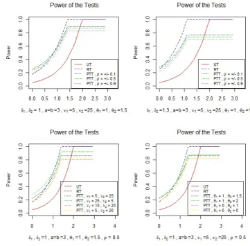
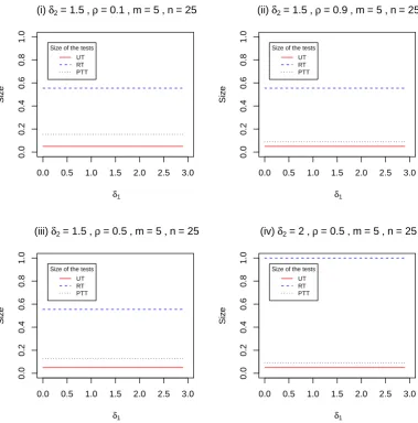
Figure 1: The power function of the UT, RT and PTT againstδ1 for some selected

0.0 0.5 1.0 1.5 2.0 2.5 3.0

0.0

0.2

0.4

0.6

0.8

1.0

(i) δ₂= 1.5, ρ = 0.1,m= 5,n= 25

δ1

Siz

e

Size of the tests UT RT PTT

0.0 0.5 1.0 1.5 2.0 2.5 3.0

0.0

0.2

0.4

0.6

0.8

1.0

(ii) δ₂= 1.5, ρ = 0.9,m= 5,n= 25

δ1

Siz

e

Size of the tests UT RT PTT

0.0 0.5 1.0 1.5 2.0 2.5 3.0

0.0

0.2

0.4

0.6

0.8

1.0

(iii) δ2= 1.5, ρ = 0.5,m= 5,n= 25

δ1

Siz

e

Size of the tests UT RT PTT

0.0 0.5 1.0 1.5 2.0 2.5 3.0

0.0

0.2

0.4

0.6

0.8

1.0

(iv) δ2= 2, ρ = 0.5,m= 5,n= 25

δ1

Siz

e

Size of the tests UT RT PTT

6

Analyses of power and size

From Figure 1, as well as from equation (4.1), it is evident that the power of the UT does not depend onδ2 and ρ, but it increases as the value of δ1 increases. The form of the power curve of the UT is concave, starting from a very small value of near zero (whenδ1 is also near 0), it approaches 1 asδ1 grows larger. The power of the UT increases rapidly as the value ofδ1 becomes larger. The minimum power of the UT is approximately 0.05 forδ1= 0.

The shape of the power curve of the RT is also concave for all values ofδ1andδ2. The power of the RT increases as the values ofδ1 and/orδ2 increase (see graphs in Figure 1(i) and 1(ii), and equation (4.2)). Moreover, the power of the RT is always larger than that of the UT for all values of δ1 and/or δ2. The minimum power of the RT is approximately 0.2 forδ1= 0 and δ2= 0. The maximum power of the RT is 1 for reasonably larger values of δ1. The power of the RT reaches 1 much faster than that of the UT asδ1 increases.

The power of the PTT depends on the values of δ1,δ2 and ρ (see Figure 1 and equation (4.4)). Like the power of the RT, the power of the PTT increases as the values ofδ1 increase. Moreover, the power of the PTT is always larger than that of the UT and RT for the values ofδ1 from around 0.7 to 1.5. The minimum power of the PTT is around 0.18 forδ1 = 0 (see Figure 1(i)), and it decreases as the value of

δ2 becomes larger. The gap between the power curves of the RT and PTT is much less than that between the UT and RT and/or UT and PTT. The power curve of the PTT tends to lie between the power curves of the UT and RT. However, the power of the PTT is identical for fixed value ofρ, regardless of its sign.

Figure 2 and equation (4.8) show that the size of the UT does not depend on

δ2. It is a constant and remains unchanged for all values of δ1 and δ2. The size of the RT increases as the value ofδ2increases (see equation (4.7)). Moreover, the size of the RT is always larger than that of the UT. The size of the UT and RT do not depend onρ.

The size of the PTT is closer to that of the UT for larger values ofδ2>2. The difference (or gap) between the size of the RT and PTT increases significantly as the value ofδ2 and ρ increases. The size of the UT is αU T = 0.05 for all values of

δ1 and δ2. For all values of δ1 and δ2, the size of the RT is larger than that of the UT,αRT > αU T. For all the values ofρ,αP T T ≤αRT. Thus, the size of the RT is always larger than that of the UT and PTT.

7

Concluding Remarks

For smaller values of δ1 (see Figure 1) the PTT has higher power than the UT and RT. But for larger values of δ1 the RT has higher power than the PTT and UT. Thus when the NSPI is reasonably accurate (that isδ1 is small) the PTT over performs the UT and RT with higher power.

Since the size of the RT is the highest, and the PTT has larger size than UT, in terms of the size the UT is the best among the three tests. However, the UT performs the worst in terms of the power. Thus the PTT ensures higher power than the UT and lower size than the RT, and hence a better choice, especially when the NSPI on the slope parameters is reasonably accurate to be close to the true values. The size of the PTT goes down as either the correlation coefficient (ρ) becomes larger (see graphs (i)-(ii) in Figure 2) or the value ofδ2increases (see graphs (iii)-(iv) in Figure 2).

References

[1] Amos, D. E. and Bulgren, W. G. (1972). Computation of a multivariate F

distribution. Journal of Mathematics of Computation,26, 255-264.

[2] Bancroft, T. A. (1944). On biases in estimation due to the use of the preliminary tests of singnificance.Annals of Mathematical Statistics,15, 190-204.

[3] Bancroft, T. A. (1964). Analysis and inference for incompletely specified models involving the use of the preliminary test(s) of singnificance.Biometrics,20(3), 427-442.

[4] El-Bassiouny, A. H. and Jones, M. C. (2009). A bivariateF distribution with marginals on arbitrary numerator and denominator degrees of freedom, and related bivariate beta andtdistributions.Statistical Methods and Applications, 18(4), 465-481.

[5] Han, C. P. and Bancroft, T. A. (1968). On pooling means when variance is unknown. Journal of American Statistical Association,63, 1333-1342.

[6] Johnson, N. L., Kotz, S. and Balakrishnan, N. (1995). Continuous univariate distributions, Vol. 2, 2nd Edition. John Wiley and Sons, Inc., New York.

[7] Judge, G. G. and Bock, M. E. (1978). The Statistical Implications of Pre-test and Stein-rule Estimators in Econoetrics. North-Holland, New York.

[8] Khan, S. (2000). Improved estimation of the mean vector for Student-t model, Communications in Statistics-Theory and Methods, 29(3), 507-527.

[9] Khan, S. (2003). Estimation of the Parameters of two Parallel Regression Lines Under Uncertain Prior Information. Biometrical Journal,44, 73-90.

[10] Khan, S. (2005). Estimation of parameters of the multivariate regression model with uncertain prior information and Student-t errors. Journal of Statistical Research,39(2), 79-94.

[11] Khan, S. (2006). Shrinkage estimation of the slope parameters of two parallel regression lines under uncertain prior information. Journal of Model Assisted and Applications,1, 195-207.

[12] Khan, S. (2008). Shrinkage estimators of intercept parameters of two simple regression models with suspected equal slopes. Communications in Statistics -Theory and Methods,37, 247-260.

[13] Khan, S. and Saleh, A. K. Md. E. (1997). Shrinkage pre-test estimator of the intercept parameter for a regression model with multivariate Student-t errors. Biometrical Journal,39, 1-17.

[15] Khan, S., Hoque, Z. and Saleh, A. K. Md. E. (2002). Estimation of the slope parameter for linear regression model with uncertain prior information,Journal of Statistical Research,36(1), 55-73.

[16] Khan, S. and Hoque, Z. (2003). Preliminary test estimators for the multivariate normal mean based on the modified W, LR and LM tests.Journal of Statistical Research, Vol 37, 43-55.

[17] Khan, S. and Saleh, A. K. Md. E. (2005). Estimation of intercept parameter for linear regression with uncertain non-sample prior information. Statistical Papers. 46, 379-394.

[18] Khan, S. and Saleh, A. K. Md. E. (2008). Estimation of slope for linear regres-sion model with uncertain prior information and Student-terror. Communica-tions in Statistics-Theory and Methods,37(16), 2564-2581.

[19] Kleinbaum, D. G., Kupper, L. L., Nizam, A. and Muller, K. E. (2008). Applied regression analysis and other multivariable methods. Duxbury, USA.

[20] Krishnaiah, P. R. (1964). On the simultaneous anova and manova tests. Part of PhD thesis, University of Minnesota.

[21] R Core Team (2013). R: A language and environment for statistical computing. R Foundation for Statistical Computing, Vienna, Austria. URL http://www.R-project.org/.

[22] Saleh, A. K. Md. E. (2006). Theory of preliminary test and Stein-type estima-tion with applicaestima-tions. John Wiley and Sons, Inc., New Jersey.

[23] Saleh, A. K. Md. E. and Sen, P. K. (1978). Nonparametric estimation of location parameter after a preliminary test on regression. Annals of Statistics,6, 154-168.

[24] Saleh, A. K. Md. E. and Sen, P. K. (1982). Shrinkage least squares estima-tion in a general multivariate linear model. Procedings of the Fifth Pannonian Symposium on Mathematical Statistics, 307-325.

[25] Schuurmann, F. J., Krishnaiah, P. R. and Chattopadhyay, A. K. (1975). Table for a multivariateF distribution.The Indian Journal of Statistics37, 308-331.

[26] Tamura, R. (1965). Nonparametric inferences with a preliminary test. Bull. Math. Stat. 11, 38-61.

[27] Yunus, R. M. (2010). Increasing power of M-test through pre-testing. Unpub-lished PhD Thesis, University of Southern Queensland, Australia.

[29] Yunus, R. M. and Khan, S. (2011a). Increasing power of the test through pre-test - a robust method.Communications in Statistics-Theory and Methods,40, 581-597.

[30] Yunus, R. M. and Khan, S. (2011b). M-tests for multivariate regression model. Journal of Nonparamatric Statistics,23, 201-218.