Spatial and environmental processes show temporal variation in the structuring of waterbird metacommunities

the structuring of waterbird metacommunities

Dominic A. W. Henry1,_{† and Graeme S. Cumming}1,2

1_{Percy FitzPatrick Institute of African Ornithology, DST/NRF Centre of Excellence, University of Cape Town, Rondebosch, Cape Town} 7701 South Africa

2_{ARC Centre of Excellence for Coral Reef Studies, James Cook University, Townsville, Queensland 4811 Australia}

Citation: Henry, D. A. W., and G. S. Cumming. 2016. Spatial and environmental processes show temporal variation in the structuring of waterbird metacommunities. Ecosphere 7(10):e01451. 10.1002/ecs2.1451

Abstract. Metacommunity theory provides a framework for assessing the role of spatial and environmental processes in structuring ecological communities and places emphasis on the role of dispersal. Four metacommunity perspectives have been proposed: species-sorting, patch dynamics, mass effects, and a neutral model. Metacommunity analysis decomposes the variance in communities into regional and local dynamics and ascribes it to one of these perspectives, although they are not always mutually exclusive. Although birds are a well- studied taxon, consensus around processes structuring freshwater avian metacommunities is lacking and few studies have repeated samples through time. We used variance partitioning to analyze waterbird community data collected over seven sampling periods at 60 wetland sites in KwaZulu- Natal, South Africa, to distinguish the processes driving beta- diversity and identify which metacommunity perspective(s) best explained these patterns. We addressed two focal questions: (1) how do environmental, spatial, and spatially structured environmental components contribute to variance in the waterbird community; and (2) given a significant contribution, which environmental variables were most important in explaining metacommunity structure? We also investigated the role of temporal variation in community processes by comparing results across sampling periods. The underlying landscape was characterized by four groups of environmental variables: vegetation structure, water quality, rainfall, and land cover. Moran’s eigenvector maps were used to generate a set of multiscale spatial predictor variables. Our results showed that the spatially structured environmental component was dominant through the sampling periods. Purely spatial and environmental components contributed a significant proportion of variance, but their magnitudes showed considerable temporal variation. Environmental processes were more pronounced in winter periods while purely spatial processes were augmented in the summer months. Our results suggest that species-sorting is the primary structuring forces in waterbird communities. The presence of spatial effects, especially in summer, does however suggest that species-sorting does not operate in isolation. Future efforts also need to address the causes and consequences of temporal variation in metacommunity processes.

Key words: metacommunity; Moran’s eigenvector maps; neutral dynamics; spatial pattern; species-sorting; temporal variation; variance partitioning; waterbirds.

Received 5 October 2015; revised 4 April 2016; accepted 26 May 2016. Corresponding Editor: C. Lepczyk.

Copyright: © 2016 Henry and Cumming. This is an open access article under the terms of the Creative Commons Attribution License, which permits use, distribution and reproduction in any medium, provided the original work is properly cited.

† E-mail: [email protected]

I

A central goal in ecology is to understand the processes that control the organization of commu-nities through space and time. The role of spatial

manner, the advancement of our understanding of metapopulation processes has been driven for-ward by incorporating ideas of dispersal and its role in maintaining connectivity between isolated populations (Hanski 1998, 1999).

The metacommunity perspective (Leibold et al. 2004) provides a productive avenue for dis-entangling the importance of various multiscale mechanisms operating on communities. A meta-community is a set of local communities that are linked, via dispersal, by an assemblage of poten-tially interacting species (Wilson 1992). There are four perspectives (species-sorting, mass effects, patch dynamics, and the neutral model) that form the basis of metacommunity theory. These four perspectives have traditionally been consid-ered separate “paradigms,” but it has recently been acknowledged that these are not as discrete as previously thought, and that metacommuni-ties are shaped by a combination of processes (Logue et al. 2011). For example, Winegardner et al. (2012) proposed that mass effects and patch dynamics are actually special cases of the species- sorting paradigm. As an alternative, the metacommunity framework can be seen as a continuum along which the species- sorting and neutral models are different endpoints of a set of processes that act on community structure. Viewing communities in this way does, however, pose challenges for empirical studies that seek to test the relative importance of the processes defined by the four perspectives.

Each metacommunity perspective advocates a different set of mechanisms by which natu-ral communities are, and have been, shaped (Leibold et al. 2004). A fundamental principle common to all of these perspectives is the ability of organisms to exhibit movement, either within or between local communities. These movements can be a response to competition, tracking of environmental change, or other dynamics which lead to either immigration into a habitat patch or emigration from a habitat patch (Leibold et al. 2004, Holyoak et al. 2005). Different perspec-tives also hold different assumptions about the relative importance of local- scale environmental conditions and spatial processes that operate at broader scales (Leibold et al. 2004).

The species- sorting perspective suggests that community composition is driven by environmen-tal characteristics and gradients while the neutral

model (Hubbell 2001) assumes that species are not fundamentally different and community composi-tion is thus determined by dispersal and spatially random events. Following this, the neutral model suggests that community dissimilarity should increase as a function of geographical distance. The mass- effect perspectives emphasize the role of both local and regional processes on community structure (i.e., a combination of both environmen-tal conditions and dispersal among sites). It shares similarities with the species- sorting model, but its predominance is filtered by independent dispersal processes (Leibold et al. 2004). The patch dynam-ics perspective, which shares characteristdynam-ics with the neutral model, assumes a high similarity in the quality of habitat patches and so all patches have an equal probability of hosting populations. In this model, community structure is driven by competition–colonization trade- offs (Leibold et al. 2004). Patch occupation may be determined by the interaction between dominant species that are superior competitors (with low dispersal abil-ity) and species which are poor competitors (with higher dispersal and colonization ability).

for thinking about slower dynamics in more sta-ble communities, metacommunity analysis offers a potentially useful approach to understanding the intersection of spatial and temporal dynamics.

Avian metacommunities provide an ideal study system because birds generally have high disper-sal capacity and are often sensitive to environ-mental change. In addition, there have been very few avian metacommunity studies—in a review of 158 data sets used for the purpose of space– environment variance partitioning (Cottenie 2005), only 3% of studies related to birds. Findings in avian studies have also supported varied meta-community paradigms; Meynard and Quinn (2008), Gianuca et al. (2013), and Özkan et al. (2013) showed that environmental variables were the predominant drivers of community structure (although at different scales) for their bird com-munities, while Driscoll and Lindenmayer (2009) found little consistent support for any of the metacommunity theories. Additionally, there is a paucity of studies which use long- term data sets to explicitly evaluate the role of temporal varia-tion in metacommunity processes.

The objective of this analysis was to assess the relative roles and importance of spatial and envi-ronmental components in structuring a waterbird metacommunity. More specifically, we aimed to distinguish the processes driving beta- diversity across network of wetlands and identify which metacommunity perspectives best explained these patterns (e.g., neutral vs. species-sorting). We addressed two primary questions: (1) What are the relative contributions of purely spatial, purely environmental, and spatially structured environmental fractions to the total explained variance of the beta- diversity of the waterbird community and how much variation in the waterbird communities can be attributed to sto-chastic variation? and (2) if purely environmen-tal explains a significant proportion of variance in the communities, which environmental vari-ables were most important in contributing to this explained variance? The analysis was then extended to investigate the role of temporal vari-ation in community structuring processes. Each sampling period was analyzed to address our two focal questions, after which comparisons were made between findings from different sam-pling periods to test whether metacommunity processes were temporally stable.

M

Analytical approach

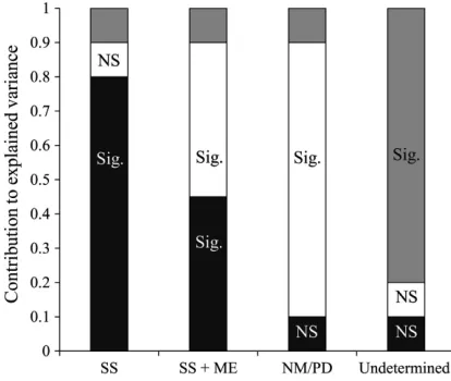
A primary aim when analyzing beta- diversity is to discriminate between sources of variation and model the relevant sources separately (Legendre et al. 2005). Variance partitioning has become a widely used and powerful approach to disentan-gle the relative roles of local environmental char-acteristics and spatial charchar-acteristics of observed beta- diversity within a study system (Legendre et al. 2005, Logue et al. 2011). Variance partition-ing then allows for decomposition of beta- diversity into three causal fractional components (Legendre et al. 2005, Peres- Neto et al. 2006): (1) purely spatial (PS), (2) purely environmental (PE), and (3) spatially structured environmental (SSE). Investigating the predominance of each of these components can then be used as a means to inform our understanding of the metacommunity processes underlying the observed beta- diversity patterns. We used variance partitioning methods to address our primary questions, and Fig. 1

provides a visual illustration of how the signifi-cance and relative contribution of variance of each component indicates a specific metacommunity process.

Study area

The study was undertaken in the northern coastal plain of KwaZulu- Natal Province, South Africa. The plain extends 170 km from the town of St Lucia in the south to the Mozambique bor-der in the north. The western and eastern bound-aries were defined by the Lebombo Mountain range and the Indian Ocean, respectively, a dis-tance of approximately 75 km. The study area is roughly 9900 km2 _{and falls within the}

Maputa-land Centre of Endemism, which is characterized by high floral and faunal diversity. The climate is subtropical with wet, hot summers, and mild winters. Annual rainfall, which is highly vari-able, ranges from 600 mm in the west to 1000 mm in the east and falls primarily in the summer months.

Accessible sampling sites were chosen to max-imize coverage over a diversity of wetlands resulting in 60 point locations incorporating 14 individual wetlands (Fig. 2). Sites were grouped according to wetland clusters. Wetlands cov-ered a wide range of hydrology, chemistry, and vegetation types including estuarine systems, freshwater endorheic lakes, a large man- made dam, floodplains, and swamps, and nutrient- rich pans. Many of the wetlands fall within national protected conservation areas, although the level of protection varies (notably, in certain wetlands protection only extends up to the high water mark, which allows people access to shore-line vegetation resources). Several wetlands are rAMSAr and Important Bird Area (IBA) sites. For full details of study area and wetland clus-ters, see Appendix S1.

Waterbird community surveys

Standardized bimonthly point counts at 60 sites across the study area were carried out from

April 2012 to June 2013. This resulted in seven sampling replicates for each of the 60 sites. All counts were carried out within the first 10 days of each sampling month. Sites were sampled in the same order throughout the majority of sampling periods. Counting commenced after a 10- min habituation period following arrival at a site in order to minimize the effect of observer distur-bance. Counts lasted 30 min and all birds were counted within a semicircle along the shoreline of 150 m radius. The distance was measured using a laser range finder. All birds were assigned to a category of either foraging, non- foraging (e.g., roosting), or flying over. Birds recorded as flying over the count site were excluded from further analysis.

Birds that are not strictly ecologically depend ent on wetlands (e.g., passerines such as sparrows that are also common in terres-trial habitats) and birds recorded in less than 10% of counts were excluded from the analy-sis. Subsequently, the analysis included 53 spe-cies from the following 15 families: Anatidae (ducks and geese), Anhingidae (darters), Ardeidae (herons and egrets), Burhinidae (thick knees), Charadriidae (plovers and lapwings), Jacanidae (jacanas), Laridae (gulls and terns), Pelecanidae (pelicans), Phalacrocoracidae (cor-morants), Phoenicopteridae (flamingos), Podi-cipedidae (grebes), rallidae (crakes and rails), recurvirostridae (stilts and avocets), Scolopacidae (sandpipers), and Threskiornithidae (ibises and

spoonbills). See Appendix S2: Table S1 for a list of waterbird species included in the analysis.

Environmental predictors

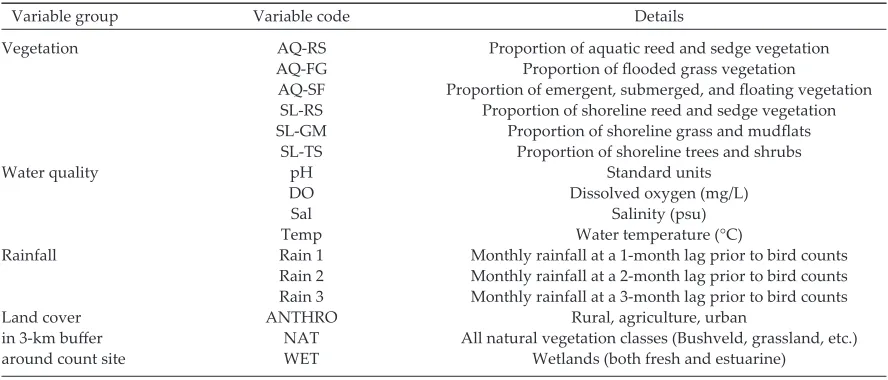
Four groups of environmental variables were measured at each site during each sampling period. These were vegetation structure (shore-line and aquatic), water quality, rainfall (at three monthly lag periods), and proportion of three land cover classes in a 3- km buffer surrounding each sampling site. For a summary of derivation and abbreviation for each variable, see Table 1.

Vegetation sampling

Vegetation structure was assessed within the count area after bird counts were completed. Vegetation structure comprised of two compo-nents: aquatic and shoreline. Aquatic vegetation cover was visually estimated by dividing the count area into four equal areas and recording the proportion of different classes (to the closest 5%) of vegetation for each segment. Three aquatic vegetation (AQ) classes were defined: (1) aquatic reeds and sedges (AQ- rS), (2) flooded grass (AQ- FG), and (3) emergent vegetation (soft stemmed plants), submerged vegetation and floating vege-tation (AQ- SF). Segments devoid of vegevege-tation were designated as open water. The total of each of these classes summed to 100%. In a similar manner, shoreline vegetation was visually esti-mated by dividing the 150 m shoreline into four segments and recording structure while walking

Table 1. Abbreviations, units, and derivations of environmental variables measured at each sampling site.

Variable group Variable code Details

Vegetation AQ- rS Proportion of aquatic reed and sedge vegetation AQ- FG Proportion of flooded grass vegetation

AQ- SF Proportion of emergent, submerged, and floating vegetation SL- rS Proportion of shoreline reed and sedge vegetation SL- GM Proportion of shoreline grass and mudflats

SL- TS Proportion of shoreline trees and shrubs

Water quality pH Standard units

DO Dissolved oxygen (mg/L)

Sal Salinity (psu)

Temp Water temperature (°C)

rainfall rain 1 Monthly rainfall at a 1- month lag prior to bird counts rain 2 Monthly rainfall at a 2- month lag prior to bird counts rain 3 Monthly rainfall at a 3- month lag prior to bird counts

Land cover ANTHrO rural, agriculture, urban

in 3- km buffer NAT All natural vegetation classes (Bushveld, grassland, etc.)

the length of the transect. Proportion of vegeta-tion was recorded within 5 m of the water’s edge. Three shoreline vegetation (SL) categories were defined: (1) shoreline reeds and sedges (SL–rS), (2) shoreline grass and mudflats (SL–GM), and (3) trees and shrubs (SL–TS). Segments which contained only rocky structure were designated as open shoreline. For a summary of vegetation structure variables across clusters, see Appendix S3: Table S1.

Water quality measurements

Water quality measurements were taken at each count site throughout the study period using a HI9828 multiparameter probe (Hanna Instruments, Cape Town, South Africa). The meter was calibrated before the start of each sam-pling period. It provided measures of pH (stan-dard units), dissolved oxygen (DO, mg/L), salinity (Sal, psu), and water temperature (Temp, °C). The probe was held about 10 cm under the surface, and five readings from each site were taken. Values for water quality variables were subsequently averaged before inclusion into the analysis. See Appendix S3: Table S2 for a sum-mary of water quality variables for each cluster. Standard deviation measures in the Mtubatuba cluster were not calculated due to the absence of water quality measurement at two of the three sites.

Rainfall

Three measures of monthly rainfall were used in this analysis. rainfall variables were calcu-lated as the total monthly rainfall in the preced-ing month (rain 1), two (rain 2), and three (rain 3) months prior to the month in which bird counts were conducted (e.g., values for sampling in April 2012: rain 1 = sum of rainfall in March 2012; rain 2 = sum of rainfall in February 2012; rain 3 = sum of rainfall in January 2012). rainfall readings were obtained from measurement sta-tions as close as possible to count sites were used. rainfall data were provided by the South African Weather Service (SAWS, www.weathersa.co.za). In the case where SAWS stations were not in close proximity to a site, or where data were missing, data were provided by Ezemvelo KZN Wildlife. See Appendix S3: Table S3 for a sum-mary of rainfall variables across sampling clusters.

Land cover

Land cover data were extracted from the 20 × 20 m resolution 2008 KwaZulu- Natal Land Cover Dataset (Ezemvelo KZN Wildlife 2011). The data were derived from SPOT5 multispectral imagery. A total of 1001 map accuracy reference points were used for groundtruthing, which resulted in 78.92% classification accuracy. Each pixel in the data set corresponds to one of 47 classes. We combined the aggregated classes to form three groups of land cover: (1) rural, agri-culture, degraded, and anthropogenically modi-fied (ANTHrO); (2) all natural vegetation (NATu); and (3) estuarine and freshwater wet-lands (WET). The proportion of these land cover classes was measured within a 3- km buffer sur-rounding each count site. Data were extracted and processed in ArcGIS version 10 (ESrI GIS software, redlands, California, uSA, www.esri. com). See Appendix S3: Table S4 for summary across clusters.

Spatial predictors

We used distance- based Moran’s eigenvector maps, MEMs (Dray et al. 2006, 2012), represent-ing spatial structures at multiple scales, to gener-ate spatial predictor variables across our network of study wetlands. MEMs are a generalized form of older methods known as principle coordinates of neighborhood matrices, PCNM (Borcard and Legendre 2002). A data- driven approach (Dray et al. 2006) was applied to community data from each sampling period independently to generate MEMs each sampling period. For a full descrip-tion of the data- driven approach to selecting MEMs, see Appendix S4.

Statistical analyses

by the spatial and environmental matrices using the adjusted R- squared (R2

adj) in rDA. The

signif-icance of the unique fraction of R2

adj (while

con-straining other fractions) for each predictor matrix as well as their combined fractions was tested for significance using Monte Carlo permu-tation tests (n = 999). Before implementing the variance partitioning, we used forward stepwise selection with a double- stopping criterion (Blanchet et al. 2008) to identify significant spa-tial and environmental variables, and included only these variables in the variance partitioning analysis as recommended by Peres- Neto and Legendre (2010). The waterbird community data matrices were Hellinger- transformed prior to inclusion in the analysis (Legendre and Gallagher 2001).

In order to address our second question, we used the R2

adj value of environmental variables

retained by the forward selection procedure to assess the relative contribution of each envi-ronmental variable to the purely envienvi-ronmental component of the variance partitioning output. All analyses were run in the r statistical software (r Core Team 2013). The spatial predictors were created using functions within the spacemaker package (Dray 2013), the stepwise selection procedure was run using the packfor package (Dray et al. 2013), and the variance partitioning was carried out using the varpart function in the vegan package (Oksanen et al. 2013).

r

Spatial weighting matrices and MEMs

Following the data- driven approach to select-ing the most suitable spatial model for each

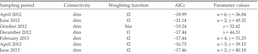
sampling period, the best spatial weighting matrix (i.e., the model with the lowest AICc) was created using the distance criterion (dnn) con-nectivity matrix (Table 2). The corresponding weighting functions selected changed through the sampling periods and included the binary weighting, linear weighting f1, and concave- down weighting f2. The full modeling outputs for spatial weighting matrices selection of each sampling period are presented in Appendix S5: Tables S1–S7. Following the selection of the most suitable spatial weighting matrices, MEM eigen-vectors were created for each sampling period. using the spatial data from April 2012 as an example (Appendix S6: Fig. S1), shows how the MEM1 corresponds to broadscale spatial pat-terns, while MEM8 shows a correspondence to fine- scale spatial patterns.

Variance partitioning

The total variance in the waterbird community explained by both spatial and environmental matrices ranged from 15.4 to 24.7% across differ-ent sampling periods (Table 3). The explained variance was significant (P < 0.05) throughout all sampling periods. Interestingly, the lower and upper bounds of this explained variance occurred in June 2013 and June 2012 sampling periods, respectively, suggesting marked differences in explanatory power of spatial and environmental variables between years. The purely environ-mental fraction of explained variance ranged from 3.0 (October 2012) to 9.5% (April 2013) and all fractions were highly significant (P < 0.05) after partialling out the effect of the spatial vari-ables (Table 3). The lowest purely environmental fractions occurred during the summer months

Table 2. results of the spatial model with the highest support, for each sampling period, following the data- driven approach for selecting the appropriate spatial weighting matrix.

Sampling period Connectivity Weighting function AICc Parameter values

April 2012 dnn f2 −18.99 α = 6; γ = 36.84

June 2012 dnn f2 −21.14 α = 2; γ = 45.32

October 2012 dnn bin −19.24 γ = 32.42

December 2012 dnn f1 −17.44 γ = 44.31

February 2013 dnn f2 −17.44 α = 4; γ = 31.25

April 2013 dnn f2 −16.75 α = 3; γ = 39.15

June 2013 dnn f2 −17.46 α = 2; γ = 40.18

(3.0, 3.6, and 4.6%). The purely spatial fraction of explained variance ranged from 0.9 (April 2013) to 7.9% (October 2012) and all fractions, except that of the April 2013 sampling period, were sig-nificant after partialling out the effect of environ-mental variables. The spatially structured environmental fraction (i.e., shared fraction between spatial and environmental variables) ranged from 6.1 (June 2013) to 12.8% (June 2012). As was the case for total explained variance, the upper and lower bounds of the SSE fraction occurred in the June months of the study period (Table 3).

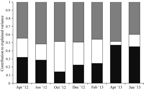
The contribution made by the SSE component to total explained variance remained fairly stable

throughout the sampling periods (range: 40–52%, Fig. 3). The PS and PE, however, showed greater differences in the magnitude of their contribu-tion throughout the sampling periods (PS range: 4–37%, PE range: 14–47%, Fig. 3). The April 2013 sampling period was unique in having the lowest PS fraction and highest PE fraction (Fig. 3).

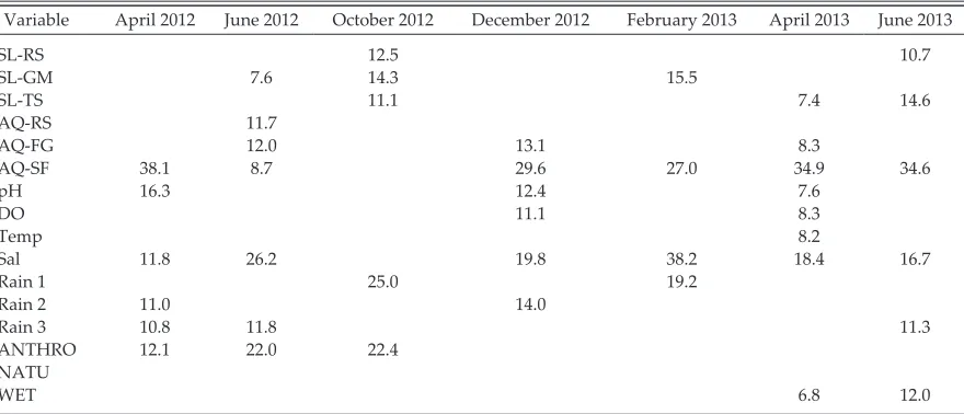
For each sampling period, several environmen-tal variables (range: 4–7) were retained after the stepwise selection procedure and were combined to represent the purely environmental component of the variance partitioning analysis (Table 4). The relative contribution to variance (measured by R2

adj) for environmental variables ranged from

6.8 to 38.2% (Table 4). For individual variables,

Table 3. Summary of the variance partitioning analyses for the waterbird metacommunity showing the per-centage of variance contributed by each component (each row is a sampling period).

Sampling period PE F df PS F df SSE Total F df

April 2012 5.6 1.61* 6, 48 4.1 1.52* 5, 48 7.8 17.5 2.14* 11, 48

June 2012 7.1 1.66* 7, 42 4.9 1.45* 7, 42 12.8 24.7 2.31* 14, 42

October 2012 3.0 1.32* 6, 44 7.9 1.59* 9, 44 10.3 21.2 2.06* 15, 44

December 2012 3.6 1.37* 6, 47 4.5 1.46* 6, 47 7.9 15.9 1.93* 12, 47

February 2013 4.6 1.74* 4, 48 5.6 1.62* 6, 48 8.6 18.8 2.34* 10, 48

April 2013 9.5 1.81* 8, 46 0.9 1.12NS _{5, 48 9.8 20.3 2.15* 13, 48}

June 2013 6.9 1.73* 6, 48 2.3 1.29* 5, 48 6.1 15.4 1.97* 11, 48

Notes: Significance of a fraction, after partialling out other effects, is shown beside the fraction value. PE, pure environmental fraction; PS, pure spatial fraction; SSE, spatially structured environmental fraction (i.e., shared spatial and environmental frac-tion); NS, non- significant fraction.

*Significant fraction (cutoff value P < 0.05).

salinity and the proportion of emergent, floating, and surface aquatic vegetation were consistently retained in all but one sampling period (October 2012). All other variables were retained in at least one sampling period model expect for propor-tion of natural vegetapropor-tion cover in the buffer sur-rounding sampling sites (Table 4).

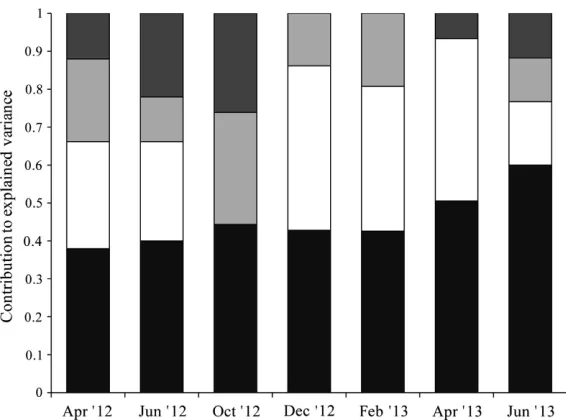
Vegetation structure consistently contrib-uted the highest proportion of variance to the purely environmental component across all sampling periods and ranged between 38.1 and 60% (Fig. 4). Water quality explained the next highest proportions of variance in all sampling periods except for in October 2012, where it did not contribute at all. The contribution from rain-fall variables varied substantially throughout the study period ranging between 0 and 25%. Land cover variables were only retained in four of the seven sampling periods and displayed a lower contribution of variance ranging from 0 to 22.4% (Fig. 4). In general, water quality was more important in the winter months while the effect of land cover was more prominent in the summer months.

d

We used the metacommunity framework to investigate the processes structuring beta- diversity of waterbird communities across a

network of wetland sites. The results of the vari-ance partitioning procedure showed that in gen-eral, all three components (PE, PS, and SSE) contributed significantly to the overall explained variance in waterbird communities, although the relative importance of each changed through the sampling periods. The SSE fraction, which is the shared fraction between space–environment variables, was the dominant (contributing on average 47% to explained variance) and most sta-ble component across all but one sampling period (June 2013). The relative contribution of PE and PS fractions changed through the sampling peri-ods. The PE fraction was consistently larger in winter months (April–September), while PS frac-tion was consistently larger in the summer months (October–March). Overall, the majority of variance explained by the various components included environmental variables. This provides support that species-sorting is the primary pro-cess structuring the waterbird metacommunity. The presence of a significant purely spatial effect, however, especially during the summer months, indicates that neutral and dispersal dynamics do indeed play a role in metacommunity structure. This result is surprising, given that waterbirds are highly mobile and that our study system lacked any significant barriers to dispersal.

Guidelines for metacommunity analysis have been proposed by Cottenie (2005), who conducted

Table 4. relative contribution (percentage of total) of variance, measured by R2

adj, of each individual

environ-mental variable in the pure environenviron-mental component of the variance partitioning.

Variable April 2012 June 2012 October 2012 December 2012 February 2013 April 2013 June 2013

SL- rS 12.5 10.7

SL- GM 7.6 14.3 15.5

SL- TS 11.1 7.4 14.6

AQ- rS 11.7

AQ- FG 12.0 13.1 8.3

AQ- SF 38.1 8.7 29.6 27.0 34.9 34.6

pH 16.3 12.4 7.6

DO 11.1 8.3

Temp 8.2

Sal 11.8 26.2 19.8 38.2 18.4 16.7

rain 1 25.0 19.2

rain 2 11.0 14.0

rain 3 10.8 11.8 11.3

ANTHrO 12.1 22.0 22.4

NATu

WET 6.8 12.0

a meta- analysis of the role of space and environ-ment characteristics in metacommunity studies. He compiled 158 data sets across multiple taxa which incorporated various scales of analysis and dispersal modes (Cottenie 2005). Variance partitioning was subsequently used to assign a metacommunity process driving the dynamics of each data set. Cottenie (2005) reasoned that when the total explained variance in beta- diversity is decomposed into a significant PE fraction and a non- significant PS fraction, the metacommunity is driven by species- sorting mechanisms. In this scenario, differences in communities relate to the presence of environmental gradients and the ability of species to exhibit a movement response in order to track these gradients. When the vari-ance is decomposed into both significant PE and PS fractions, then species- sorting and mass- effect processes will operate. Cottenie (2005) and Leibold et al. (2004) pointed out that the patch dynamic perspective incorporates a spatial com-ponent generated by immigration and emigra-tion dispersal events, in which species face a competition–dispersal trade- off (i.e., individuals can avoid competitive exclusion by immigrating into areas where they are good competitors). This pattern is therefore the result of a purely spatial

signal which is independent of environmental conditions (Cottenie 2005). In a system that is completely devoid of a significant PE component and only consists of a PS component, neutral model processes (Hubbell 2001) will operate such that because species and habitat are assumed to be similar, only dispersal processes will generate spatial patterns (Cottenie 2005).

Following this reasoning, our results suggest that species-sorting was the dominant process operating on the waterbird metacommunity in the April 2013 sampling period, while a combination of species- sorting and dispersal processes (incor-porated into mass effects) was dominant through-out the rest of the study period. In accordance with our findings, the results of Cottenie’s (2005) meta- analysis revealed that species-sorting was a domi-nant mechanism operating across a wide range of taxa and ecological systems. This result does not, however, negate spatial dispersal processes which also play a role. Indeed, the next most prevalent metacommunity type stemmed from a combina-tion of species-sorting and mass effects, which is what our results suggest through the majority of our sampling periods. Interestingly, the large SSE fraction in our study opposed the findings of Cottenie (2005), in which this component ranked

Fig. 4. The relative contribution of variance (measured by R2

adj) by each group of environmental variables in

lowest in explaining community variation. The SSE fraction is caused by induced spatial depen-dence which strengthens the importance of envi-ronmental component. The large contribution of the SSE fraction in our study does, however, restrict the ability to make conclusions about metacommunity processes with absolute cer-tainty. This discrepancy between our findings and those of Cottenie (2005) could be due to three lim-iting factors of the meta- analysis. First, Cottenie (2005) used third- order polynomials of geograph-ical coordinates to model the spatial component, which have been shown to be inferior to the newer MEM methods (Dray et al. 2006, 2012) that are able to model spatial variation at multiple scales. This could possibly have lead to a failure to ade-quately detect spatial patterns and hence down-play the role of spatial processes. Second, the data were only obtained from studies conducted in northern temperate regions. While we cannot be sure that these processes do not differ across ecosystems, the origin of the data may limit the ability to make general inferences for processes operating in tropical regions, such as our study site. Third, very few of the study systems included birds as the focal study organisms (the majority of studies focussed on macroinvertebrates and zooplankton). However, findings of other studies of avian metacommunities generally do support species- sorting mechanisms as a dominant force (Barbaro et al. 2007, Meynard and Quinn 2008, Sattler et al. 2010, Gianuca et al. 2013, Özkan et al. 2013, Bonthoux and Balent 2015), although some studies do report either a lack of stable metacom-munity processes (Driscoll and Lindenmayer 2009) or evidence of neutral dynamics (White and Hurlbert 2010, Meynard et al. 2011).

The variation in the prominence of PE (winter) and PS (summer) indicated that seasonal dynam-ics of both species and the landscape need to be understood in order to gain a deeper understand-ing of the temporally stable components structur-ing metacommunities. The change in importance of variance partitioning components could be due to two factors. First, the majority of precipitation occurs in the summer months which coincide with the breeding period of resident waterbirds (Hockey et al. 2005). This causes a change in the type and configuration of resources; in addition to permanent waterbodies, smaller ephemeral wetlands may form part of the landscape. These

productive habitats are often used by breeding waterbirds. Assuming that the availability of wet-lands is limiting, a greater PS weighting might be related to the dispersal of waterbirds which are seeking out suitable breeding habitats and territo-ries. Competition for these high- quality ephemeral habitats might strengthen the effect of interspe-cific competition which would, in turn, alter local population dynamics (Holyoak et al. 2005, Gotelli et al. 2010). Second, the concurrent influx of non- breeding migrant waterbirds during summer may also serve to amplify this spatial signal. Significant numbers of Palearctic migrants arrive in the aus-tral summer and integrate across a semiarid land-scape in which wetlands are patchy and dynamic. This increase in abundance may strengthen com-petitive forces, as resident species who are seek-ing out high- quality habitat necessary to meet the requirements of breeding come into contact with migrant species. Spatial processes which empha-size dispersal and colonization– competitive abil-ity may therefore play a more prominent role during these periods and reduce the variation attributed to purely environmental factors. In a temporal study on the metacommunity dynamics of stream fishes in Hungary, Eros et al. (2012) also found substantial variation in the relative contri-bution of PS, PE, and SSE to total explained vari-ance. This pattern could be attributed to changes in hydrology and water chemistry, which can act at fine temporal scales in river systems.

incorporate temporal patterns (e.g., extension of eigenvector methods, such as MEMs, to analyze multivariate time- series data).

In addressing the second question, our results showed that vegetation structure variables (espe-cially aquatic surface and emergent vegetation) contributed the largest amount of variance to the portion of purely environmental component. This contribution was relatively stable through sampling periods. Water quality variables were the next most important explanatory variables, particularly salinity. Apart from vegetation struc-ture, the contribution from the remaining three environmental variable groups showed marked variation through sampling periods. It is reason-able to expect the observed variation for rainfall and water quality, both of which can be driven by dynamics operating at fine temporal scales. It was, therefore, surprising that land cover (in which measurements did not change throughout the sampling period) showed a similar dynamic. Aquatic vegetation structure and salinity played important roles because of their ability to dis-criminate between wetlands with opposing char-acteristics and waterbird assemblages. These results reinforce the importance of aquatic mac-rophytes and water quality as drivers of habitat use by waterbirds (Balcombe et al. 2005, russell et al. 2009, Terörde and Turpie 2013).

There are inherent limitations in our study that bear mentioning. First, the potential weakness of using variance partitioning to detect and differ-entiate between metacommunity processes has been pointed out (Smith and Lundholm 2010). Second, Chang et al. (2013) showed that the conclusions drawn about metacommunities can depend heavily on the choice of environmental variables included in the analysis. The presence of a high PS, as found in our study, may be the result of unmeasured spatially structured envi-ronmental variables. However, the relationships between variables included in this analysis and waterbirds are well established—for example, for water quality (Halse et al. 1993, Ashkenazi 2001, Kalejta- Summers et al. 2001, Cumming et al. 2013), vegetation structure (Murkin et al. 1997, raeside et al. 2007, russell et al. 2009), and rainfall (roshier et al. 2002, 2008, Kingsford et al. 2010). While it is nearly impossible to include all environmental variables relevant in the ecological niche of a study organism, the choice of variables

here is appropriate for addressing metacommu-nity hypotheses. The total explained variance in our sampling periods was moderate; these values were on par with, and in some instances higher, than those in other similar studies (Sattler et al. 2010). unexplained variation could be attributed to stochastic processes (e.g., the effect of anthro-pogenic disturbance at a particular site) influ-encing our study system, but despite the high variance in spatiotemporal dynamics of wetlands in the southern African landscape coupled with the high mobility of waterbirds, this value was not excessively high.

Given the relatively low number of studies explicitly addressing metacommunity processes in wetland bird communities, this study makes an important contribution to understanding how assemblages are structured across a large network of wetlands. Species- sorting and mass- effect dynamics appear to be the dominant and most important drivers of community structure in waterbirds. Our findings regarding the rele-vance of spatial components do however suggest that species- sorting dynamics do not operate in isolation. Our results also highlight the utility of analyzing metacommunity dynamics in multiple sampling periods and have shown the relative importance of spatial and environmental pro-cesses can vary significantly through time. Future research should focus on unraveling how envi-ronmental change and social dynamics contrib-ute to temporal variance in community patterns.

A

This research was supported by a GAINS (Global Avian Influenza Network for Surveillance) subcon-tract from uSAID, via the Wildlife Conservation Society, to GC. Additional funding was provided by the DST/NrF Centre of Excellence at the Percy FitzPatrick Institute, an NrF Incentive Grant to GC, and the university of Cape Town. We would like to thank David Nkosi, Chevonne reynolds, and Justin Henry for their help in conducting bird and vegetation surveys. Thank you to the staff at Ezemvelo KZN Wildlife and iSiMangaliso Wetland Park for assistance with field site access and logistics.

l

c

Balcombe, C. K., J. T. Anderson, r. H. Fortney, and W. S. Kordek. 2005. Vegetation, invertebrate, and wildlife community rankings and habitat analysis of mitigation wetlands in West Virginia. Wetlands Ecology and Management 13:517–530.

Barbaro, L., J.-P. rossi, F. Vetillard, J. Nezan, and H. Jactel. 2007. The spatial distribution of birds and carabid beetles in pine plantation forests: the role of landscape composition and structure. Journal of Biogeography 34:652–664.

Blanchet, F. G., P. Legendre, and D. Borcard. 2008. For-ward selection of explanatory variables. Ecology 89:2623–2632.

Bonthoux, S., and G. Balent. 2015. Bird metacommu-nity processes remain constant after 25 years of landscape changes. Ecological Complexity 21: 39–43.

Borcard, D., and P. Legendre. 2002. All- scale spatial analysis of ecological data by means of principal coordinates of neighbour matrices. Ecological Modelling 153:51–68.

Borcard, D., P. Legendre, and P. Drapeau. 1992. Partial-ling out the spatial component of ecological varia-tion. Ecology 73:1045–1055.

Chang, L. W., D. Zelený, C. F. Li, S. T. Chiu, and C. F. Hsieh. 2013. Better environmental data may reverse conclusions about niche- and dispersal- based processes in community assembly. Ecology 94:2145–2151.

Cottenie, K. 2005. Integrating environmental and spa-tial processes in ecological community dynamics. Ecology Letters 8:1175–1182.

Cumming, G. S., M. Ndlovu, G. L. Mutumi, and P. A. r. Hockey. 2013. responses of an African wading bird community to resource pulses are related to foraging guild and food- web position. Freshwater Biology 58:79–87.

Dray, S. 2013. spacemaker: Spatial modelling. r pack-age version 0.0-5/r113. https://r-forge.r-project.org/ r/?group_id=195

Dray, S., P. Legendre, and F. G. Blanchet. 2013. packfor: forward selection with permutation (Canoco p.46). r package version 0.0-8/r109. https://r-forge.r-proj ect.org/r/?group_id=195

Dray, S., P. Legendre, and P. r. Peres-Neto. 2006. Spa-tial modelling: a comprehensive framework for principal coordinate analysis of neighbour matri-ces (PCNM). Ecological Modelling 196:483–493. Dray, S., r. Pélissier, and P. Couteron. 2012.

Commu-nity ecology in the age of multivariate multiscale spatial analysis. Ecological Monographs 82:257– 275.

Driscoll, D. A., and D. B. Lindenmayer. 2009. Empirical tests of metacommunity theory using an isolation gradient. Ecological Monographs 79:485–501.

Eros, T., P. Sály, P. Takács, A. Specziár, and P. Bíró. 2012. Temporal variability in the spatial and environ-mental determinants of functional metacommu-nity organization: stream fish in a human- modified landscape. Freshwater Biology 57:1914–1928. Ezemvelo KZN Wildlife. 2011. KwaZulu-Natal Land

Cover 2008 V1.1. unpublished GIS Coverage (Clp_ KZN_2008_LC_V1_1_grid_w31.zip), Biodiversity Conservation Planning Division, Ezemvelo KZN Wildlife, Cascades, Pietermaritzburg, South Africa. Gianuca, A. T., V. A. G. Bastazini, r. A. Dias, and M. I.

M. Hernández. 2013. Independent and shared effects of environmental features and space driv-ing avian community beta diversity across a coastal gradient in Southern Brazil. Austral Ecol-ogy 38:864–873.

Gotelli, N. J., G. r. Graves, and C. rahbek. 2010. Mac-roecological signals of species interactions in the Danish avifauna. Proceedings of the National Academy of Sciences of the united States of Amer-ica 107:5030–5035.

Halse, S. A., M. r. Williams, r. P. Jaensch, and J. A. Lane. 1993. Wetland characteristics and waterbird use of wetlands in south- western Australia. Wild-life research 201:103–125.

Hanski, I. 1998. Metapopulation dynamics. Nature 396:41–49.

Hanski, I. A. 1999. Metapopulation ecology. Oxford university Press, Oxford, uK.

Hockey, P. A. r., W. r. J. Dean, and P. ryan, editors. 2005. roberts birds of Southern Africa. Seventh edition. Trustees of the John Voelcker Bird Book Fund, Cape Town, South Africa.

Holyoak, M., M. Leibold, and r. Holt. 2005. Metamunities: spatial dynamics and ecological com-munities. university of Chicago Press, Chicago, Illinois, uSA.

Houlahan, J. E., et al. 2007. Compensatory dynamics are rare in natural ecological communities. Pro-ceedings of the National Academy of Sciences of the united States of America 104:3273–3277. Hubbell, S. 2001. The unified neutral theory of

biodi-versity and biogeography. Princeton unibiodi-versity Press, Princeton, New Jersey, uSA.

Kalejta-Summers, B., M. McCarthy, and L. G. under-hill. 2001. Long- term trends, seasonal abundance and energy consumption of waterbirds at Strand-fontein, Western Cape, South Africa, 1953–1993. Ostrich 72:80–95.

Kingsford, r., D. roshier, and J. Porter. 2010. Aus-tralian waterbirds: time and space travellers in dynamic desert landscapes. Marine and Fresh-water research 61:875–884.

variation of community composition data. Ecologi-cal Monographs 75:435–450.

Legendre, P., and E. D. Gallagher. 2001. Ecologically meaningful transformations for ordination of spe-cies data. Oecologia 129:271–280.

Legendre, P., and O. Gauthier. 2014. Statistical meth-ods for temporal and space–time analysis of com-munity composition data. Proceedings of the royal Society B 281:20132728.

Leibold, M. A., et al. 2004. The metacommunity concept: a framework for multi- scale community ecology. Ecology Letters 7:601–613.

Levin, S. A. 1992. The problem of pattern and scale in ecology: the robert H. MacArthur award lecture. Ecology 73:1943–1967.

Logue, J. B., N. Mouquet, H. Peter, and H. Hillebrand. 2011. Empirical approaches to metacommunities: a review and comparison with theory. Trends in Ecology & Evolution 26:482–491.

MacArthur, r. H., and E. O. Wilson. 1967. The theory of island biogeography. Princeton university Press, Princeton, New Jersey, uSA.

Meynard, C. N., V. Devictor, D. Mouillot, W. Thuiller, F. Jiguet, and N. Mouquet. 2011. Beyond tax-onomic diversity patterns: How do α, β and γ

components of bird functional and phylogenetic diversity respond to environmental gradients across France? Global Ecology and Biogeography 20:893–903.

Meynard, C. N., and J. F. Quinn. 2008. Bird metacom-munities in temperate South American forest: veg-etation structure, area, and climate effects. Ecology 89:981–990.

Murkin, H. r., E. J. Murkin, and J. P. Ball. 1997. Avian habitat selection and prairie wetland dynamics: a 10- year experiment. Ecological Applications 7:1144–1159.

Oksanen, J., et al. 2013. vegan: community ecology pack-age. r package version 2.0-9. https://cran.r-project. org/web/packages/vegan/index.html

Özkan, K., J. C. Svenning, and E. Jeppesen. 2013. Envi-ronmental species sorting dominates forest- bird community assembly across scales. Journal of Animal Ecology 82:266–274.

Peres-Neto, P. r., and P. Legendre. 2010. Estimating and controlling for spatial structure in the study of ecological communities. Global Ecology and Biogeography 19:174–184.

Peres-Neto, P. r., P. Legendre, S. Dray, and D. Borcard. 2006. Variation partitioning of species data matrices: estimation and comparison of fractions. Ecology 87:2614–2625.

r Core Team. 2013. r: a language and environment for statistical computing. r Foundation for Statistical Computing, Vienna, Austria. http://www.r-project. org/

raeside, A. A., S. A. Petrie, and T. D. Nudds. 2007. Waterfowl abundance and diversity in relation to season, wetland characteristics and land- use in semi- arid South Africa. African Zoology 42:80–90. roshier, D. A., A. I. robertson, and r. T. Kingsford.

2002. responses of waterbirds to flooding in an arid region of Australia and implications for con-servation. Biological Conservation 106:399–411. roshier, D. A., V. A. Doerr, and E. D. Doerr. 2008.

Ani-mal movement in dynamic landscapes: interaction between behavioural strategies and resource distri-butions. Oecologia 156:465–477.

russell, I. A., r. M. randall, B. M. randall, and N. Hane-kom. 2009. relationships between the biomass of waterfowl and submerged macrophytes in a South African estuarine lake system. Ostrich 80:35–41. Sattler, A. T., D. Borcard, r. Arlettaz, F. Bontadina,

P. Legendre, and M. K. Obrist. 2010. Spider, bee, and bird communities in cities are shaped by envi-ronmental control and high stochasticity. Ecology 91:3343–3353.

Smith, T. W., and J. T. Lundholm. 2010. Variation parti-tioning as a tool to distinguish between niche and neutral processes. Ecography 33:648–655.

Terörde, A. I., and J. K. Turpie. 2013. Influence of hab-itat structure and mouth dynamics on avifauna of intermittently- open estuaries: a study of four small South African estuaries. Estuarine, Coastal and Shelf Science 125:10–19.

White, E. P., and A. H. Hurlbert. 2010. The combined influence of the local environment and regional enrichment on bird species richness. American Naturalist 175:E35–E43.

Wilson, D. S. 1992. Complex interactions in metacom-munities, with implications for biodiversity and higher levels of selection. Ecology 73:1984–2000. Winegardner, A. K., B. K. Jones, I. S. y. Ng, T. Siqueira,

and K. Cottenie. 2012. The terminology of meta-community ecology. Trends in Ecology & Evolu-tion 27:253–254.

s

I