Reducing Latencies in Earthquake Early Warning

(1)

Thesis by

Lucy Yin

In Partial Fulfillment of the Requirements for the degree of

Doctor of Philosophy

CALIFORNIA INSTITUTE OF TECHNOLOGY

Pasadena, California

2018

(2)

Lucy Yin

(3)

To my father and Wentao

(4)

ACKNOWLEDGEMENTS

The memorable years at Caltech have forever changed my life in numerous ways. The pursuit of my PhD degree was only possible with the support and assistance from the Caltech faculty, scientists, friends, and family. There are too many people to thank.

First and foremost, I would like to acknowledge my advisor Professor Tom Heaton. I am very grateful for his help throughout the time at Caltech. Working with him has been a great privilege and also very enjoyable. His inspiring ideas always guide me to think outside of box and be a creative innovator. What I learned from him is far beyond the knowledge of engineering seismology. In addition to his academic guidance, he has supported me during the emotionally tough times and gave me moral support. He is not only my academic advisor at Caltech; he is also my advisor in life.

I want to express my sincere gratitude to my thesis advising committee, Prof Domniki Asimaki, Prof Jean-Paul Ampuero, Prof Yisong Yue, and Dr Morgan Page, for the time they dedicated to my thesis and research progress. I learned so much from them, from seismology to applied mathematics, to statistics, and to computer science. I would also like to thank Prof Jim Mori and Prof Masumi Yamada for their hospitality during my visit to Kyoto University. Not only did I enjoy participating in the English seismology seminars, but also I will never forget the memories of Gion Matsuri, hanabi, and mushi atsui weather. I am grateful to have worked with all the researchers and scientists from the EEW group, especially my collaborators Dr Men-Andrin Meier and Dr Jennifer Andrews. I thank them for their insights during our discussions and the effort and time put into our manuscripts.

(5)

Karakus, Dr. Stephen Wu, Dr Ming Hei Cheng, and Dr Ramses Mourhatch, who taught me the survival strategies through PhD.

My heartfelt gratitude goes to my parents, Dr. John Jiahong Yin and Mrs. Ellen Guirong Tang, who support me with their unconditional love. Ever since I can remember, my father always inspired me to pursue my dreams in the academic path. And for my mom, I hope that she could see my accomplishment from heaven, and keep watching over me as my guardian angel. Lastly, I would like to thank Dr. Wentao Huang for always being on my side during the journey at Caltech. I am forever grateful for his love, patience, understanding and encouragement helping me going through the ups and downs. I look forward to the next adventurous chapter of our lives together away from Caltech.

I would also like to acknowledge the financial support from the Natural Science and Engineering Research Council of Canada (NSERC) through their postgraduate doctoral and master’s scholarships (PGS), and the Gordon and Betty Moore Foundation.

(6)

ABSTRACT

Existing Earthquake Early Warning (EEW) algorithms use waveform analysis for earthquake detections, estimation of source parameters (i.e., magnitude and hypocenter location), and prediction of peak ground motions at sites near the source. The latency of warning delivery due to data collection significantly restricts the usefulness of the system, especially for users in the vicinity of the earthquake source, as the warning may not arrive before the strong shaking. This presentation discusses several methods to reduce the warning latency, while maintaining reliability and robustness, so that the warning time can be maximized for users to take appropriate actions to reduce causalities and economic losses.

Firstly, we incorporated the seismicity forecast information from Epidemic-Type Aftershock Sequence (ETAS) model into EEW as prior information, under the Bayesian probabilistic inference framework. Similar to human’s decision-making process, the Bayesian approach updates the probability of the estimations as more information becomes available. This allows us to reduce the required time for reliable earthquake signal detection from at least 3 seconds to 0.5 second. Furthermore, the initial error of hypocenter location estimation is reduced by 58%. The performance of the algorithm is further improved during aftershock sequences and swarm earthquakes.

(7)

(8)

PUBLISHED CONTENT AND CONTRIBUTIONS

Yin, L., M. Meier, and T. Heaton (2017), “Making earthquake early warning faster and more accurate using ETAS seismicity models as a Bayesian prior”, 16th world Conference on Earthquake Engineering proceeding, N 2850

Yin, L., J. Andrews, and T. Heaton, “Rapid Earthquake Discrimination for Earthquake Early Warning: A Bayesian Probabilistic Approach using Three-Component Single Station Waveforms and Seismicity Forecast”, The Bulletin of the Seismological Society of America (under review)

(9)

LIST OF ILLUSTRATIONS AND/OR TABLES

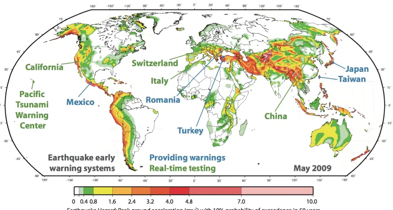
Figure 1.1 Seismic hazard map and countries where EEW is in operation or being tested under development by May 2009 (Allen, Gasparini, et al. 2009) ... 5

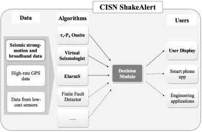
Figure 1.2 Framework of CISN ShakeAlert. The bold modules with solid lines are the existing system that is currently running. The dashed lines show components under development. (Bose, Allen, et al. 2014) ... 8

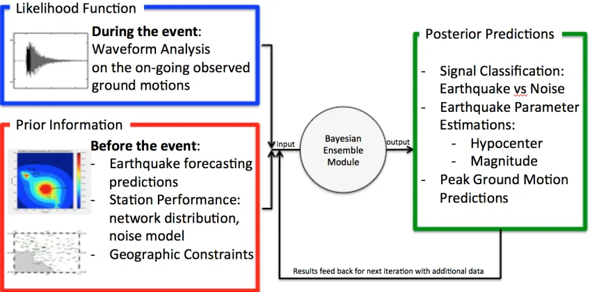
Figure 1.3 Flow Chart of Bayesian framework in EEW ... 9

Figure 2.1 Time frame of various earthquake information products ... 14

Figure 2.2 Four simulation results of the Northridge aftershock for a 24-hour period of January 18 -19, 1994 calculated by Felzer ETAS model ... 19

Figure 2.3 Average result of the Felzer ETAS model simulation after 50 runs ... 20

Figure 2.4 Average result of the Felzer ETAS model simulation after 500 runs ... 20

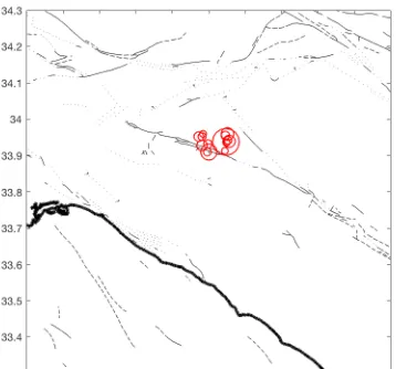
Figure 2.5 Modified ETAS forecast map for Chino Hills earthquake sequence on 29 July 2008 ... 24

Figure 2.6 Observed seismicity of Chino Hills earthquake sequence on 29 July 2008. The size of the red circle scale with observed magnitude of the earthquake records. ... 24

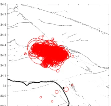
Figure 2.7 Modified ETAS forecast map for Northridge earthquake sequence on 17 April 1994 ... 25

(14)

Figure 2.9 Modified ETAS forecast map for Cucapah El Mayor Sequence on 9 April 201026

Figure 2.10 Observed seismicity of Cucapah El Mayor Sequence on 9 April 2010. The size of the red circle scale with observed magnitude of the earthquake records ... 26

Figure 2.11 Modified ETAS forecast map for a seismic dormant region during 13 May 2015 ... 27

Figure 2.12 Observed seismicity of a seismic dormant region during 13 May 2015. The size of the red circle scale with observed magnitude of the earthquake records. ... 27

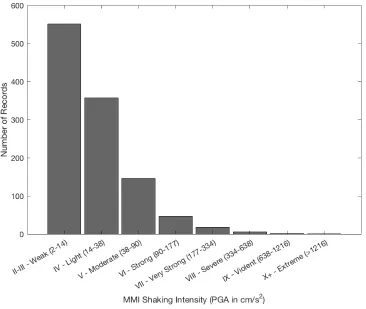
Figure 3.1 MMI shaking intensity distributions of the 1,128 earthquake records collected for the study ... 32

Figure 3.2 Maximum ground motion amplitude distributions collected for every half-second window within the initial 3.0s after the trigger time of all 2,481 three-component records used for this study. The labeled earthquake data are earthquake records with PGA greater than 2cm/s2; noise data are false triggers including calibration pulses, jumps in electric current, glitches induced by machinery, and ambient noise; the teleseism data include 353 records from 14 teleseismic events. The lines are the fitted Gaussian distributions to earthquake (solid), noise (dash) and teleseism (dot dash) data. The notations are A=acceleration, V=velocity, Z=vertical, H=horizontal. ... 35

Figure 3.3 First and updated predictions at the initial 3 sec of the p-wave arrival ... 38

(15)

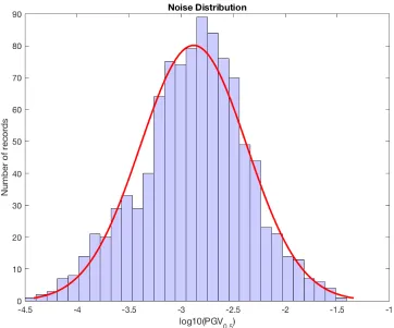
Figure 3.5 Histogram of the vertical log10(PGV) at the 0.5s after trigger from the 1000

noise data randomly sampled from 100 most noisiest stations across the network during 2015 ... 53

Figure 3.6 Visual explanation of two-tailed p-value computation under Normal Distribution55

Figure 3.7 Seismicity rate calculation in a flow chart ... 57

Figure 3.8 Source to station Distance Calculation based on the initial p-wave amplitude observed at the station ... 58

Figure 3.9 Magnitude calculation at the sources based on the initial p-wave amplitude observed at the station ... 59

Figure 3.10 Seismicity rate calculation obtained from the ETAS model ... 59

Figure 3.11 Comparison of the predictive results from waveform analysis, Bayesian model with simple prior, and Bayesian model with modified prior at 0.5sec after station trigger. ... 62

Figure 3.12 Comparison of the predictive results from waveform analysis, Bayesian model with simple prior, and Bayesian model with modified prior at 1.5sec after station trigger. ... 62

Figure 3.13 Comparison of the predictive results from waveform analysis, Bayesian model with simple prior, and Bayesian model with modified prior at 3.0 sec after station trigger. ... 63

(16)

Figure 3.15 Precision rate (%) for waveform analysis, Bayesian model with simple prior, and Bayesian model with modified prior as a function of time. ... 65

Figure 3.16 Flow chart of the proposed signal discrimination process for real-time implementation ... 66

Figure 3.17 MMI Shaking Intensity for the missed earthquake events at a) 0.5 s and b) 3.0 s after triggered time ... 68

Figure 3.18 τc-Pd plot of all earthquake and non-earthquake (noise and teleseism) data in our data set using a 3.0 s window following the P-wave trigger for measurement. The solid line and dashed line are the decision boundaries of the parameter Q=1 and Q=0.5, respectively. The color intensity of the earthquake data represents the PGA observed ... 70

Figure 3.19 initial 3.0 sec vertical acceleration waveform and prediction results for stations CI.CFS and CI.NEN during ambient noise false triggers on 24 March 2015 ... 73

Figure 3.20 Map of M3.7 Chino Hill Aftershock: hypocenter in the yellow star and locations of CI.OLI and CI.LBW1 in red triangles ... 74

Figure 3.21 initial 3.0 sec vertical acceleration waveform and prediction results for stations CI.OLI and CI.LBW1 during M3.7 Chino Hill aftershock on 27 July 2008 ... 75

Figure 3.22 Map of M 4.7 Los Angeles earthquake: hypocenter in the yellow star and locations of CI.WNS and CI.MIS in red triangles ... 76

(17)

Figure 3.24 Initial 3.0 sec vertical acceleration waveform and prediction results for stations CI.SMR and CI.SMW during M7.8 Japan Teleseismic earthquake on 30 May 2015.79

Figure 4.1 Catalog location of the 506 target M4.0+ earthquakes in Southern California from 1990 to 2015. Including 2009 Lone Pine M5.2 Earthquake in red star and 2008 Chino Hills M5.4 Earthquake in yellow star. ... 87

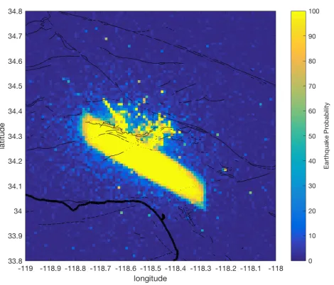
Figure 4.2 Seismicity Forecast Map for Lone Pine M 5.2 Earthquake. It was produced immediately after the first station trigger at CI.CGO. The intersection of the two blue lines is the catalog location ... 89

Figure 4.3 Probabilistic location estimation map of the M5.2 Lone Pine Earthquake at various times after the first station trigger. a) c) and e) are results of Gutenberg Algorithm at 0.5 sec, 5.5 sec, and 10.5 sec after the first trigger, respectively. b) d) and f) are posterior results of Gutenberg Algorithm with Prior at 0.5 sec, 5.5 sec, and 10.5 sec after the first trigger, respectively. The intersection of the two blue lines is the catalog location. ... 90

Figure 4.4 M5.2 Lone Pine Earthquake location error as a function of time after the origin time. The blue and red lines are the location error results of the Gutenberg Algorithm, and the Gutenberg Algorithm with ETAS Prior, respectively. ... 91

Figure 4.5 Seismicity Forecast Map for Chino Hills M 5.4 Earthquake. It was produced immediately after the first station trigger at CI.CHN. The intersection of the two blue lines is the catalog location ... 93

(18)

and 1.5 sec after the first trigger, respectively. The intersection of the two blue lines is the catalog location. ... 94

Figure 4.7 M5.4 Chino Hills Earthquake location error as a function of time after the origin time. The blue and red lines are the location error results of the GbA and GbA with ETAS Prior, respectively. ... 95

Figure 4.8 Location Error as a function of time after first trigger for 506 M4+ earthquakes in Southern California 1990-2015 a) likelihood performance: GA results b) posterior performance: GA with Prior results. The errors are specified at the 25th, 50th, 75th, and 95th percentile ... 97

Figure 5.1 A 2-dimensional KD tree example: a) visual distribution of the database in feature dimensions, b) tree structure of the database. A database of 10 earthquake records (A - J) is organized using KD tree data structure (grey lines are the branches of the tree). As a new waveform is recorded, the target record (yellow star) only needs to visit 5 of the data points (red points) to find the record with the most similar record with respect to the select features: initial 3 sec velocity and acceleration of the p-wave. In the KD tree method, only the data points with branches that intersect the hypersphere (shaded circle) are possible candidates; being closer than the current nearest node, other nodes (blue points) can be ignored. As a comparison, the linear sequential search requires going through all 10 records, which doubles the computation effort. ... 108

(19)

Figure 5.3 Ground motion residuals for the 500-validation dataset with different database sizes. Peak Ground Velocity residuals are given in absolute ground motion units. The lines show the percentile according to the legend. The 50th percentile is the average residual error; the 100th and 0th percentiles indicate the maximum and minimum errors respectively. ... 112

Figure 5.4 Ground motion residuals for the 500-validation dataset with different database sizes. Peak Ground Displacement residuals are given in absolute ground motion units. The lines show the percentile according to the legend. The 50th percentile is the average residual error; the 100th and 0th percentiles indicate the maximum and minimum errors respectively. ... 113

Figure 5.5 Source parameter residual for the 500-validation dataset with different database size. Magnitude residuals are given in absolute units. The lines show the percentile according to the legend. The 50th percentile is the average residual error; the 100th and 0th percentiles indicate the maximum error and minimum error respectively. 114

Figure 5.6 Source parameter residual for the 500-validation dataset with different database size. Hypocenter distance residuals are given in absolute units. The lines show the percentile according to the legend. The 50th_{percentile is the average residual error;}

the 100th_{and 0}th_{percentiles indicate the maximum error and minimum error}

respectively. ... 115

Figure 5.7 CPU searching time for different database sizes using linear sequential search and KD tree search. The implementation is in Matlab. ... 117

(20)

Figure 6.1 Noise amplitude records from a few selected Community Seismic Network stations (provided by the CISN research group) ... 126

Table 2.1 EEW decision-making scenarios under Bayesian framework ... 16

Table 3.1 The teleseism events obtained in this study. Strong-motion sensors in Southern California record all these events. ... 34

Table 3.2 Coefficient parameters calculated using the MLE method, as well as accuracy and precision measures for all candidate models. ... 40

Table 3.3 Waveform Analysis mode performance at time increments: 0.5s, 1.0s, 1.5s, 2.0s, 2.5s, 3.0s after the triggered time at the station ... 41

Table 3.4 Model performance of the Bayesain model with a simple prior at time increments: 0.5s, 1.0s, 1.5s, 2.0s, 2.5s, 3.0s after the triggered time at the station .. 48

Table 3.5 Model performance of the Bayesian model with a modified prior at time increments: 0.5 s, 1.0 s, 1.5 s, 2.0 s, 2.5s, 3.0 s after the triggered time at the station61

Table 3.6 Cross-validation confusion matrix ... 67

Table 3.7 Comparison results of the proposed method with τc-Pd method. ... 71

(21)

(22)

C h a p t e r 1

Introduction

1.1

Motivation

An earthquake is a natural disaster that develops over a very short time frame; the time interval between the initial of rupture to the end of damaging ground motion arriving at a site could be from the order of seconds to a minute. However, the aftermath damage that an earthquake brings could be permanent and significant. Scientists, the government and the private sector have put in tons of effort in mitigating earthquake losses. Although earthquake prediction is a challenging task, the development of Earthquake Early Warning (EEW) systems has progressed rapidly over the past few decades (Allen, Gasparini, et al. 2009).

The advancement of Earthquake Early Warning systems has been driven by the growth of information technology and the increase of awareness of seismic hazard. The goal of Earthquake Early Warning is to provide alerts to the community about the incoming ground shaking and take appropriate actions to save lives and reduce losses. Strauss and Allen 2016 have estimated that EEW could decrease the number of injuries during an earthquake by more than 50%, and reduce millions of dollars in economic savings from fire damage, semiconductor plant danger, and train collisions, with statistically three lives rescued annually. The obvious benefits of the application have brought the attention of researchers worldwide to develop and implement EEW systems.

(23)

in the final updates (unfortunately, sometimes come after the arrival of the strongest shaking), the uncertainties in the earliest alerts could be largely due to the lack of available ground motion data (Bose, Allen, et al. 2014). In principal, there is a trade-off between accuracy and time: as more data is collected from the observation of the on-going earthquake with the progress of time, the analysis can produce more accurate estimations. However, warnings would be delayed if significant time was necessary for data collection. The earliest alerts are the most critical outcomes of the system because the strongest shaking is generally experienced near the earthquake hypocenter where the propagated seismic waves arrive earliest. To overcome the challenge of latency and accurate predictions, in this thesis we propose several methodologies to maximize warning time (for earliest alerts) while guaranteeing a robust accuracy level of the messages.

The latency for warning times in EEW,∆𝑡_!"#$%&', is defined as:

∆𝑡_!"#$%&' = ∆𝑡_!"#"+∆𝑡_!"#+∆𝑡_!"#$% [1.1]

where ∆𝑡!"#" is the time necessary to collect sufficient ground motion stream data, ∆𝑡!"#is

the time needed to estimate parameters about the earthquake (such as magnitude, location or predicted ground motion), and ∆𝑡_!"#$% is the time required to transmit the alert information to the community. Since ∆𝑡_!"#$% highly depends on the hardware device and the allowable bandwidth of information transmission, it is out of the research scope for seismologists. In fact, ∆𝑡!"#$% can be minimized to the order of fraction of seconds

(24)

minimize ∆𝑡_!"#", I propose to incorporate prior information data, so that additional data can be collected simultaneously. As data from various independent sources are obtained in parallel, required observations can be gathered with less time. Chapters 2 through 4 of the thesis focus on the formulation and collection of prior information from earthquake forecasting; and then apply the Bayesian probabilistic approach to combine the seismic knowledge from different sources under an ensemble model to provide final predictions. To reduce ∆𝑡_!"#, I present a data structure organization method, multidimensional binary search (KD Tree) to efficiently query desired estimations in order in Chapter 5.

From hardware deployment to algorithm development, from decision making to public education, EEW involves contributions among different scientific and engineering communities. As an earthquake engineer, my goal is to reduce the damage brought by disasters to the minimum through the efforts to develop intelligent algorithms. Only by improving the accuracy and speed of the future alert, can the system reach its full potential in performance.

1.2 Background on Earthquake Early Warning System (EEW)

1.2.1 EEW concept and development

(25)

delivered immediately after detecting the first earthquake signals at a seismic station. The speed of the more damaging S-waves from earthquakes is about 3.5km/s, whereas electrically transmitted signals from the seismic network sensors travel at about 3.0x105km/s. As the seismic waves propagate, the seismometers observe more streams of the real-time ground motion data. As a result, the real-time analysis of the earthquake parameters becomes more precise. The characterized information on the event is then delivered to the users of EEW. The warning time, as defined by the duration between the EEW alert received by the user and the arrival of strong shaking at the user’s site, needs to be sufficient to respond with appropriate actions. In general, the warning time increases as the latency time decreases. In addition to the scientific effort to reduce the warning latency, many inevitable geological factors that could dominate the latency include the distance between the site and the hypocenter, depth of the earthquake source, and soil properties, etc.

(26)

consequences in the societal adoption of EEW. It is critical for scientists and engineers to collaborate in developing robust and reliable EEW systems that provide timely alerts with guaranteed accuracy.

1.2.2 Overview of earthquake early warning systems around the world

Although the concept of earthquake early warning has been around for awhile (since (Cooper 1868)), the implementation of the systems has been achieved only over the past few decades with the development of necessary instruments, computational power, and network communications. EEW systems have been in operation in several regions around the world (Normile 2004). Figure 1.1 shows a seismic hazard map and countries where EEW is in operation or being tested (Allen, Gasparini, et al. 2009).

[image:26.612.134.530.415.627.2]

(27)

Japan has implemented one of the first applications of EEW. In the late 1960s, the Japan Railway (JR) has started monitoring ground shaking by deploying seismometers near their Bullet Train, also named as Shikansen, train tracks. The power of the Bullet Train is automatically shut off if the ground shaking intensity achieves a threshold of 40 gals. (Nakamura and Tucker 1988). The system was upgraded to the Urgent Earthquake Detection and Alarm System (UrEDAS) in the 1980s. Additional seismometers are deployed along the costal lines to provide more warning time for the trains (Nakamura 1984). The system worked well during the Niigata Chuestu earthquake in 2004, applying brakes to the Bullet Train within 3 sec after the detection of p-wave arrival (Nakamura, et al. 2006). Currently, the Japan Meteorological Agency is able to broadcast national wide public warnings of on-going earthquakes by television, cellphone, and other means of telecommunications (Doi 2003).

The Seismic Alert System (SAS) for Mexico City was established after the 1985 Michoaca earthquake (J. Espinosa-Aranda, et al. 1995). The SAS was the first public warning system in the world. Seismometers are deployed along the coastal line, located about 300km southwest of Mexico City, to detect subduction earthquake. The system is effective because the subduction zone is a few hundreds of kilometers away from Mexico City, so warnings can be provided to the city about 60 sec prior to the arrival of the damaging seismic waves (Lee and Espinosa-Aranda 2003) (J. Espinosa-Aranda, et al. 1996). Due to the high population density and soft soil properties of Mexico City, the SAS system provides very useful information for the departments in charge of emergency services.

(28)

estimate the earthquake magnitude (Wu, et al. 2006). Studies have shown that the system could provide 20 s of warning time to Taipei if the 1999 Chi-chi earthquake reoccurs (Wu and Kanamori 2005).

(29)

Figure 1.2 Framework of CISN ShakeAlert. The bold modules with solid lines are the existing system that is currently running. The dashed lines show components under development. (Bose, Allen, et al. 2014)

[image:29.612.131.524.137.394.2]

(30)

1.2.3 Bayes’ Theorem for EEW

[image:30.612.114.538.426.636.2]

Bayesian Probabilistic approach to Earthquake Early Warning was first introduced in the Virtual Seismologist method (Cua 2005). The application of Bayes’ theorem the probability of source characterization at any given time of the on-going earthquake, is a combination results from prior information and contributions from the available ground motion observations. The main differentiation of the Bayesian approach from other EEW algorithms is the exploitation of knowledge from previous experience or judgments that are not generally incorporated in automated decision-making process. A flow chart of Bayesian approach for EEW is shown in Figure 1.3. This methodology mimics the human ability to process many types of information simultaneously, combining the analyzed results to make a final decision at the end, and updating the decision over time as additional information is collected.

(31)

The inspiration of such a decision making process in earthquake early warning comes from human beings’ judgments on weather. For example, if a person needs to decide on bringing an umbrella outside, one would look at the weather forecast information and check if there are water drops outside the window. During this process, the person’s brain is performing a Bayesian calculation: the weather forecast information provides a prior information of how probable the region is going to rain in general, and the actual observation water drop is a likelihood collection of the rain probability. The goal of my thesis is to apply a similar approach of this elegant concept to earthquake early warning, so information from multiple heterogeneous sources can be processed in parallel to make fast and reliable decisions.

The prior information in earthquake early warning systems includes recent seismicity rates, distribution of seismometer network, health status of the stations, and regional seismic hazard risk, etc. For example, earthquakes tend to be active near geologic faults, so for long-term predictions, the probability of earthquake occurrence is higher near the recognized faults. Also, earthquakes tend to cluster in space and time, forming a foreshock-mainshock-aftershock sequence, so recent seismic activities are good indications of near future seismicity. In Chapter 2 of this thesis, I present a detailed formulation of an earthquake forecasting model.

The general Bayes’ theorem for EEW can be expressed as a product of the prior probability density function, 𝑃 𝐴 , multiplied by the likelihood probability density function, 𝑃 𝐵 𝐴 ,

and normalized by the evidence function, 𝑃 𝐵 , shown as the follows:

𝑃 𝐴 𝐵 =𝑃 𝐵 𝐴 𝑃(𝐴)

𝑃(𝐵)

∝𝑃 𝐵 𝐴 𝑃(𝐴)

(32)

where 𝐴 is the parameter we are interested in estimate (in EEW, this includes signal discrimination of earthquake source vs. noise source, regression estimation of source parameters such as magnitude and hypocenter location, prediction of peak ground motion intensities at users’ sites, etc.), and 𝐵 is the given incoming observations (in EEW, this includes on-going ground motion observation data, such as time-series data of waveforms, GPS displacement, etc.). 𝑃 𝐴 𝐵 is the posterior probability density function, meaning the probability of A given the observation data B. The evidence function 𝑃 𝐵 is the probability of the observation data that is independent of the estimating parameter 𝐴. This term is normalization constant, which does not affect the estimation of the parameter 𝐴, so the posterior function is proportional to the product of the likelihood function and the prior function.

Depending on the prediction task, the Bayesian framework can be applied to different estimating parameter and the predictive term 𝐴 is replaced with the parameter of interest. In the earthquake detection problem, Eq [1.2] becomes:

𝑃 𝑌 =𝐸𝑞 𝑆(𝑡) ∝𝑃 𝑆 𝑡 𝑌= 𝐸𝑞 𝑃(𝑌=𝐸𝑞) [1.3]

where 𝑌 =𝐸𝑞 is estimating the signal source being an earthquake event, and 𝑆 𝑡 is the avalaible ground motion observation at time 𝑡.

Similarly, in estimating the hypocenter location, the Eq [1.2] becomes:

𝑃 𝐿𝑎𝑡,𝐿𝑜𝑛 𝑆(𝑡) ∝𝑃 𝑆 𝑡 𝐿𝑎𝑡,𝐿𝑜𝑛 𝑃(𝐿𝑎𝑡,𝐿𝑜𝑛) [1.4]

where (𝐿𝑎𝑡,𝐿𝑜𝑛) is estimating the coordinate location of the earthquake source, and 𝑆 𝑡

(33)

Although the framework for different tasks is similar, the detailed constructions for the predictive functions vary dramatically. In Chapter 3 and 4 of this thesis, I present detailed approaches in answering both of the questions.

1.3 Research goal and Thesis plan

In order to construct an early warning system with faster initial alerts while maintaining the accuracy of the predictive information, we introduce methodologies from the seismology domain knowledge and computer science techniques to incorporate additional useful predictive information and efficiently organize large seismic database, respectively. The objectives of this thesis include:

- Reduce latency time for first early warning alert

- Improve accuracy of the earthquake parameter estimations - Minimize process delays of large databases

(34)

C h a p t e r 2

Earthquake Forecasting Methods

2.1

Background on Foreshock

-

Mainshock

-

Aftershock Sequences

Many seismologists have observed the temporal and spatial clustering properties of earthquakes (Kagan and Jackson 1991) (M. Bouchon, et al. 2013) (Gerstenberger, et al. 2005). This clustering pattern is often referred as foreshock – mainshock – aftershock sequences. The term “aftershock” is often defined as a series of smaller earthquakes following a “mainshock”, which is an earthquake with larger magnitude. “Foreshock” is the smaller earthquakes that occurred prior to the mainshock in time. Of course, sometimes the predefined mainshock could produce aftershocks for years and the aftershocks produced may be larger than the mainshock (Lomnitz 1966), while other times, not all premonitory events are observed prior to large earthquakes (Abercrombie and Mori 1996). In addition, another type of seismic activity with location clustering pattern is the swarm earthquake (Shearer 2012), which occurs repeatitively over time at the same location.

(35)

Although the science behind earthquake formulation is complex and controversial, most scientists agree on the clustering properties of earthquake occurrences. No matter what the true explanation is behind the science of earthquake sequences, one conclusion is indisputable: the recent seismicity is a good indication of seismic activities of the near future.

2.2

Earthquake Forecasting and Earthquake Early Warning

As proposed in the Bayesian approach to earthquake early warning system, prior information can be incorporated to provide faster and more accurate warnings. Earthquake early warning, earthquake forecasting, and seismic hazard maps all provide a forecast of future earthquake occurrences, evaluated for different time frames. Figure 2.1 shows the relative time frame for the three earthquake information products.

Figure 2.1 Time frame of various earthquake information products

(36)

make automated decisions and take immediate action to avoid losses from the disaster, as shown in Chapter 1. The conventional concept of EEW is to send out warnings after detecting an initial seismic wave, so the analysis sorely depends on the observation of the on-going earthquake and not previously observed seismicity.

Earthquake forecasting tends to predict regional seismicity activities in the near future based on the recent seismicity. In this model, the recent change in seismicity is the major influence of model predictions. Scientists often use the forecasting models to predict aftershock patterns of a particular seismic sequence. However, they can be applied for any region or time of interest in general. This model is often created for the prediction range of the next few hours to months.

Lastly, seismic hazard maps are intended to provide insight to the general public and guidance in development. The input of this model is based on the long-term historical seismic occurrence that has lasted for years. The information provided from hazard maps is essential in creating and updating seismic designs provisions of building codes and facilitate government on urban planning. In general, the seismic hazard maps forecast the regional hazard level for the next few years to decades.

(37)

Warning in Southern California 2009)), and this process is repeated for every earthquake event. However, in the cases when we are expecting high seismicity, such as during aftershock sequences or swarm earthquakes, it is unnecessary to redundantly wait until the end of the data collection process to send out the alert because the new trigger is probably due to another aftershock earthquake in the sequence.

In such cases, the alerts can arrive much faster to the users near the source to mitigate potential dangers from the disaster. Table 2.1 shows the decision-making scenarios under Bayesian inference, where immediate decisions can be made when consistent predictions from waveform analysis and seismic forecast are observed. The earthquake forecasting models can provide the expected seismicity information necessary in the early warning system. Of course, the large earthquakes do not always occur when the expected seismicity is high; waiting is still required to collect additional data in these cases.

High earthquake probability from waveform analysis

Low earthquake probability from waveform analysis

High earthquake probability

from seismic forecast Send alert immediately

Wait for additional waveform analysis

Low earthquake probability from seismic forecast

Wait for additional

waveform analysis No alert immediately

(38)

Since EEW system aims to provide information to all earthquakes causing ground motions that could be dangerous, alerts should be issued faster for all earthquakes during the entire sequence including aftershocks, and not only emphasize the system performance during a large magnitude mainshock. During aftershocks, the repetitive ground shaking continuously deteriorates already weakened infrastructure components. Additional natural disasters, such as landslides and tsunami, can also be triggered from aftershocks as a consequence. The seismic damage can be even more significant if the aftershocks occur close to a populated urban area. The benefits of a rapid and reliable EEW system during the aftershocks of a large earthquake are equally (or more, in some cases) important than the mainshock, as rescue and repair personals are continuously working in then already damaged and fragile epicentral region (Bakun, et al. 1994). For example, over 200 aftershocks occurred after the single mainshock during the Northridge earthquake sequence. There is also a chance that what seemed like a recent mainshock turns out to be foreshock activity of another large event (Reasenberg and Jones, Earthquake Hazard After a Mainshock in California 1989), like the 1992 M6.5 Big Bear Earthquake occurring three hours after the M7.3 Landers Earthquake. If the prior information can assist in sending out faster alerts for all the aftershock events, then system performance would be improved for over 99% of all events.

2.3

General Epidemic-Type Aftershock Sequence (ETAS) model

(39)

from other aftershock simulation methods. These secondary aftershocks are true observations in the real earthquake sequences (Felzer, Becker, et al. 2002). This statistical method quantitatively describes the clustering property in earthquake sequence processes and the generated earthquakes that have the probability of generating secondary earthquakes. The construction of the model suggests that the distribution of aftershocks follows the Omori’s Law in time (Utsu 1961), Gutenberg-Richter relationship in magnitude (Gutenberg and Richter 1944) and mainshock-aftershock distance relationships.

Taking the ETAS simulation created by Felzer (K. Felzer, Stochastic ETAS aftershock simulator 2007) as an example, the magnitude and location of the aftershocks are sampled from the distributions, and the primary aftershocks are fed back into the model to produce the secondary aftershocks; this process repeats. The generated aftershocks that match the time period and region of interested are selected to create a report of aftershock catalog. Every run of the simulation will produce different results due to the randomness of the sampling procedure. The maximum likelihood estimation (MLE) of aftershock locations can be calculated by running the simulation hundreds or thousands of times and taking the average results of all the simulations.

(40)

[image:40.612.127.518.121.472.2]

Figure 2.2 Four simulation results of the Northridge aftershock for a 24-hour period of January 18 -19, 1994 calculated by Felzer ETAS model

(41)

[image:41.612.207.442.142.343.2]

Figure 2.3 Average result of the Felzer ETAS model simulation after 50 runs

[image:41.612.207.441.433.634.2]

(42)

We can run the simulation repetitively and then get an average result for the earthquake-forecasting map. However, the computational delay introduced is not tolerable for real-time seismicity application of Earthquake Early Warning system. For example, a 50-run takes about 1 min on Matlab platform; the 500-run takes about 5 minutes. Started with the fundamental concept of ETAS simulation by (K. Felzer, Stochastic ETAS aftershock simulator 2007), I created an ETAS forecasting model that produces a MLE of earthquake forecasting map with a single run of negligible computational delay time about a single second. The real-time ETAS model can be incorporated into EEW upon the instantaneous requirements.

2.4 Modified

Epidemic

-

Type Aftershock Sequence (ETAS) model

The forecast earthquake probability calculated using an ETAS seismicity model is based on the premise that the location of future earthquakes is significantly influenced by the accumulation of previously observed earthquakes. The concept of the ETAS seismicity model has been well established in the earthquake-forecasting field and the forecasting results have been validated through many earthquake sequences (Y. Ogata 1998) (K. Felzer 2009). The future earthquake occurrence process is modeled as a nonhomogeneous Poisson process in time; the probability of one or more earthquakes occurring above 𝑀!"# at

location 𝑙𝑎𝑡,𝑙𝑜𝑛 within the time range Δ𝑡_is:

𝑝𝑟𝑜𝑏!"#$ 𝑙𝑎𝑡,𝑙𝑜𝑛 = 1−𝑒𝑥𝑝 𝜆 𝑡,𝑙𝑎𝑡,𝑙𝑜𝑛 𝑑𝑡

!!∆!

!

(43)

where 𝜆 𝑡,𝑙𝑎𝑡,𝑙𝑜𝑛 is the forecast rate of earthquake at current time t and location (lat, lon). It is composed of the long-term background seismicity 𝜇 𝑙𝑎𝑡,𝑙𝑜𝑛 _{and the short-term}

observed seismicity.

𝜆 𝑡,𝑙𝑎𝑡,𝑙𝑜𝑛 = 𝜇 𝑙𝑎𝑡,𝑙𝑜𝑛 + 𝜆_! 𝑡,𝑙𝑎𝑡,𝑙𝑜𝑛

! [2.2]

I model earthquake sequences following Omori’s Law in time (Utsu 1961), Gutenberg-Richter's relationship in magnitude (Gutenberg and Richter 1944) and Felzer and Brodsky's relation (Felzer and Brodsky 2006) in space. The short-term seismicity rate caused by each of the historical earthquakes in the catalogue is first calculated as a function of a distance from the hypocenter source,𝜆_! 𝑡,𝑟 , and then mapped to latitude and longitude,

𝜆_! 𝑡,𝑙𝑎𝑡,𝑙𝑜𝑛 , using a numerical transformation based on the distance-to-location mapping

on the earth surface. The formulation for the seismicity rate by 𝑗th earthquake at the current time 𝑡 and distance 𝑟 km is:

𝜆! 𝑡,𝑟 =

𝐾_!10! !!!!!"#

𝑡−𝑡_!+𝑐 !𝑟! [2.3]

where 𝐾_! =0.008,𝛼 =1,𝑐 =0.095,𝑝 =1.34,𝑛 = 1.37are ETAS model parameters of California obtained from (K. Felzer 2009) and 𝑙𝑎𝑡_!,𝑙𝑜𝑛_!,𝑀_! are source parameters of the

𝑗th earthquake from the observed seismicity catalog. 𝑀_!"# is the minimum magnitude of the forecast earthquakes. In the application of this proposed method to EEW, I assume that the EEW system has the access to the seismicity catalog record that continuously updates with time. As time passes, all the newly occurred events should automatically concluded in the catalog for the forecasting of future events.

(44)

(45)

[image:45.612.234.413.426.593.2]

Figure 2.5 Modified ETAS forecast map for Chino Hills earthquake sequence on 29 July 2008

Figure 2.6 Observed seismicity of Chino Hills earthquake sequence on 29 July 2008. The size of the red circle scale with

(46)

[image:46.612.234.414.424.595.2]

Figure 2.7 Modified ETAS forecast map for Northridge earthquake sequence on 17 April 1994

Figure 2.8 Observed seismicity of Northridge earthquake sequence on 17 April 1994. The size of the red circle scale with

(47)

Figure 2.9 Modified ETAS forecast map for Cucapah El Mayor Sequence on 9 April 2010

Figure 2.10 Observed seismicity of Cucapah El Mayor Sequence on 9 April 2010. The size of the red circle scale with observed

(48)

Figure 2.11 Modified ETAS forecast map for a seismic dormant region during 13 May 2015

Figure 2.12 Observed seismicity of a seismic dormant region during 13 May 2015. The size of the red circle scale with

(49)

2.5 Summary

This chapter discusses the earthquake clustering properties in time and space, forming foreshock-mainshock-aftershock sequences. Furthermore, I presented methods to forecast near future earthquakes, especially the Epidemic-type Aftershock Sequence (ETAS) model. ETAS model predicts future seismicity based on statistical models of aftershock relationships. The seismic forecasting information brings significant insights to early warning systems. Despite the size of the earthquakes, most of the seismicity activities we observe are aftershocks of a sequence. Therefore, the previously observed earthquakes are good indications of near future events. I implemented an ETAS forecast model that provides real-time solution while maintaining the accuracy.

(50)

C h a p t e r 3

3. ETAS Prior application one: Rapid Earthquake

Discrimination

3.1 Introduction

Due to the rapid advancement of digital seismic networks, Earthquake Early Warning (EEW) systems are currently able to analyze the real-time ground motion information and have the potential to provide warnings to potential users before strong shaking begins (Heaton 1985) (Allen and Kanamori 2003). We desire these EEW systems to provide both reliable and fast alerts, however, the goals of accuracy and speed are often in conflict with each other. Since the arrival of the destructive S-wave follows closely after the arrival of the P-wave in the epicentral region, processing delays must be minimized if we hope to provide warnings of the potentially damaging S-waves near an earthquake’s epicenter.

(51)

by an earthquake source, and different criteria have been imposed to filter out the non-earthquake triggers: the single-station Onsite algorithm collects and analyzes a fixed window of 3s before declaring an event (Bose, Hauksson, et al., A Trigger Criterion for Improved Real-Time Performance of Onsite Earthquake Early Warning in Southern California 2009); network-based algorithms require a minimum number of triggered stations for warning confirmation (e.g. Elarms-2 requires 4 stations for California (Kuyuk and Allen 2014), and Presto requires 3-5 stations for Southern Italy (Satriano, et al. 2011)). These methods can introduce a significant delay, especially in regions with low station density.

In this chapter, three predictive models are presented to identify earthquake source signals. First, a waveform analysis model uses a logistic regression method to predict the probability of incoming signals being generated by earthquake or non-earthquake sources. Then, two Bayesian models are presented that employ earthquake forecasting results (from Chapter 2) in addition to the waveform analysis model. One model uses the peak ETAS probability of the region as the Bayesian prior, and the other uses a derived earthquake probability from the ETAS model and noise distribution as the Bayesian prior.

3.2 Method and Data

(52)

performed to demonstrate the robustness of the model in future predictions; 3) the proposed method is compared with the existing 𝜏_!-𝑃_! method to assess speed and accuracy gains; and 4) we demonstrate the application of the method in several test cases: an earthquake mainshock, an aftershock, an ambient noise false trigger, and a teleseismic event.

3.2.1 Data

We collected three component strong-motion waveforms from local crustal earthquake and non-earthquake records in the southern California region to train the prediction model to identify earthquake signals. The non-earthquake records include ambient noise signals and teleseismic events that were detected by STA-LTA-type triggering at single seismic stations. All the strong-motion traces, 2,481 three-component records in total, are downloaded from the Southern California Earthquake Data Center. The station trigger times are provided by the Onsite algorithm (Kanamori 2005) (Y. Wu, et al. 2007) and are calculated using the modified characteristic function developed by R. Allen, 1978.

(53)

2010), the M5.4 La Habra (28 March 2014) and the M5.4 Borrego Springs (7 July 2010) earthquakes. The majority of the records in the study created weak to light shaking. Although these records are minor concerns for the purpose of large earthquakes or human sensitivity, it is necessary to include them for a complete description of the statistical population of observations of an EEW system, since low PGA values are more often recorded due to the natural distribution of earthquake occurrence and ground motion attenuation with distance. A better identification of the low PGA earthquake records improves the overall performance of the earthquake detection.

[image:53.612.137.503.328.637.2]

(54)

The data set of non-earthquake records consists of, 1000 noise and 353 teleseismic records. The noise signals include calibration pulses, jumps in electric current, glitches induced by machinery, ambient noise, etc. Since the total number of false triggers is on the scale of millions per year, the noise records were uniformly sampled from the top 100 noisiest stations in the CI network during 2015 (as observed by the Onsite algorithm STA-LTA triggering) to capture the general characteristics of noise disturbances most likely to mistakenly trigger the seismic network. The teleseism data set comprises records from 14 teleseismic events that triggered the Southern California seismic stations between 2008 and 2015. Table 3.1 shows the list of teleseismic events obtained in this study.

Time Region Latitude Longitude Depth (km) Magnitude

2008-02-21 Nevada,USA 41.15 -114.87 6.7 6.0

2010-02-27 Offshore

Bio-Bio, Chile

-35.9 -72.73 35 8.8

2010-08-18 Mariana Islands 12.2 141.51 10 6.3

2011-03-11 Tohoku, Japan 38.30 142.37 30 9.0

2012-04-12 Gulf of

California

28.79 -113.14 10.3 6.9

2012-08-14 Sea of Okhotsk 49.78 145.13 625.9 7.7

2012-12-14 Offshore Baja

California

31.09 -119.66 13 6.3

2013-02-06 Solomon

Islands

-10.80 165.114 24 8.0

2013-05-24 Sea of Okhotsk 54.89 153.22 598.1 8.3

2014-03-05 Vanuate -14.42 169.54 648 6.3

2014-04-01 Iquique, Chile -19.6 70.77 25 8.2

2014-06-23 Raoul Island, New Zealand

-29.98 177.73 20 6.9

2014-06-29 New Mexico,

USA

32.582 -109.17 6.4 5.3

2014-06-29 Samoa Islands -14.9 -175.4 10 6.5

(55)

Japan

Table 3.1 The teleseism events obtained in this study. Strong-motion sensors in Southern California record all these events.

3.2.2 Data Processing and Feature Extraction

For each baseline-corrected record, the acceleration and velocity in the vertical and horizontal directions are processed. The acceleration records are directly obtained after removal of the trend and bias of the raw data; the velocity records are obtained by integrating the acceleration data in the time domain, and then applying a fourth-order causal Butterworth high pass filter with a corner frequency of 0.075Hz. This filter is applied recursively in the time domain, so the processed time is negligible. The horizontal records are calculated using the square root of the sum of the squares of the two horizontal components.

(56)

sophisticated Bayesian model selection methods can be also applied to extract the useful features; this is beyond the scope of this study.

These features of the ith record at the kth half-second time window after the triggered time

are combined into a vector

𝑋!,! = [1,𝑙𝑜𝑔!" 𝑍𝑎!,! ,𝑙𝑜𝑔!" 𝐻𝑎!,! ,𝑙𝑜𝑔!" 𝑍𝑣!,! ,𝑙𝑜𝑔!" 𝐻𝑣!,! ] , where 𝐻 and 𝑍

denote horizontal and vertical component, and 𝐴 and 𝑉 denote acceleration and velocity, respectively. We also label ith record 𝑌𝑖 =1 or 𝑌𝑖= −1 for earthquake and non-earthquake records, respectively. Note both noise and teleseismic records are considered as non-earthquake records.

(57)

including calibration pulses, jumps in electric current, glitches induced by machinery, and ambient noise; the teleseism data include 353 records from 14 teleseismic events. The lines are the fitted Gaussian distributions to earthquake (solid), noise (dash) and teleseism (dot dash) data. The notations are A=acceleration, V=velocity, Z=vertical, H=horizontal.

3

.3

Waveform

A

nalysis

In waveform analysis, the goal is to predict the probability of the observed signal being caused by an earthquake source given only the available waveform information,

𝑝𝑟𝑜𝑏 𝑌!|𝑋!,!!:!! . We defined the classification result for station 𝑖 as 𝑌! =1 as an

earthquake record and 𝑌_! = −1 as a non-earthquake record.𝑋_!,!_!_:!_! is the waveform input

of station 𝑖 recorded during time 𝑡_!to 𝑡_!. In general, 𝑡_!is the p-wave arrival time at the station; this is when the model starts to record the ground motion data for the predictions.

By assuming that the observed data 𝑋_!_,_!_!:!!follows an independent and identically

distributed random variable, the Bayesian equation can be written as:

𝑝𝑟𝑜𝑏 𝑌! =1|𝑋!,!!:!! ∝ 𝑝𝑟𝑜𝑏 𝑌! = 1|𝑋!,!!

!

!!!

[3.1]

(58)

𝑝r𝑜𝑏 𝑌_! = 1|𝑋_!_,_!_! =𝜙 𝑋_! = 1

1+𝑒!! !!,!_! [3.2]

where

𝑓 𝑋_!_,_!_! =𝑐_!𝑥_!_!_,_!_!+𝑐_!𝑥_!_!_,!_!+⋯+𝑐_!𝑥_!",_!_! = 𝜃_!𝑥_!",!_! = 𝜃∙𝑋_!!_,_!_!

!

!!!

[3.3]

𝑥_!"_,_!_! is the 𝑗th measurement of log of the ground motion during the kth half-second time

window after triggered time at the 𝑖th station, 𝑚is the total number of measurements, and

𝜃! is the 𝑗th model parameter. Let 𝑋!,!! = 𝑥!",!!,𝑥!!,!!,𝑥!!,!!,…,𝑥!",!! , and 𝜃 = 𝑐!,𝑐!,…,𝑐! . The model parameters are determined from the training data set described

earlier. In our study, we focus on four measurements of ground motion: vertical acceleration, horizontal acceleration, vertical velocity, and horizontal velocity. The best combination of features is chosen for 𝑋_!_,!_!are based on the performance of model selection,

details in the following section. According to this convention, as 𝑓 𝑋_!,_!_! deviates further

from 0 in the positive direction; the signal is more likely to be cause by an EEW-relevant earthquake source. The predicted probability of Eq[3.2] approaches one indicates that the event is very likely to be caused by an earthquake source; it also implies that the probability of detecting a non-earthquake source approaches zero, and vice versa in the opposite direction as 𝑓 𝑋_! deviates from 0 to the negative direction.

(59)

Figure 3.3 First and updated predictions at the initial 3 sec of the p-wave arrival

3.3.1 Determination of the Model Parameters

Although the framework of the model is determined, the appropriate model parameters 𝜃 in the predictive formula from Eq[3.3] need to be specified to be useful to make predictions. To focus attention on the parameters of the likelihood function, we apply the Maximum Likelihood Estimation (MLE) method to determine the coefficients of the logistic regression that classifies earthquake and non-earthquake data. Classification methods such as Fisher’s linear discriminant analysis (LDA) and the Least Squares estimates are alternative approaches to obtain the model coefficients. However, unlike the MLE method, these classification models do not provide a probabilistic interpretation to its predictive classes, which makes it challenging to measure the degree of uncertainties.

The MLE method can be interpreted as searching for an estimation of 𝜃 that best fit of the training data we collected. Assuming that all 𝐷_!" are sampled independently and identically

Pick time

First

(60)

from the distribution, the optimal model parameters 𝜃 conditioned on the data 𝐷_!" =

𝑋!,!!,𝑌!,!! : 𝑖=1…𝑚,𝑘= 1…𝑛 can be expressed as:

𝜃 =𝑎𝑟𝑔𝑚𝑎𝑥 𝑝𝑟𝑜𝑏 𝐷_!"|𝜃 = 𝑎𝑟𝑔𝑚𝑎𝑥 𝑝𝑟𝑜𝑏 𝐷_!"|𝜃 ! !!! ! !!! [3.4] where

𝑝𝑟𝑜𝑏 𝐷!"|𝜃 =

1

1+𝑒!!!! !!,!_!|! [3.5]

where 𝑚 =2481 is the total number of waveform records in the training, including earthquake, noise, and teleseism; 𝑛 = 6 is the number of half-second windows in the initial 3.0 sec after triggered time.

3.3.2 Model Selection

Applying the MLE method, we determined the model parameter coefficients for all 15 combinations of the four ground motion features using the training dataset. Table 3.2 demonstrates the model parameters and performance of all the candidate models. We focus on two performance measures for the model selection given the following definitions:

• True Positives (TP): true predicted earthquake data • True Negatives (TN): true predicted non-earthquake data

• False Positives (FP): false predicted earthquake data, also referred to as false alerts

• False Negatives (FN): false predicted non-earthquake data, also referred to as missed events

(61)

𝑃𝑟𝑒𝑐𝑖𝑠𝑖𝑜𝑛 % = 𝑇𝑃

𝑇𝑃+𝐹𝑃 [3.6]

at 0.5 sec after the trigger. A higher precision rate indicates a lower false alerts rate. This avoids modifications or cancelations of events that could potentially confuse the system and users. Secondly, we evaluate the final accuracy rate, defined as:

𝐴𝑐𝑐𝑢𝑟𝑎𝑐𝑦 % = 𝑇𝑃+𝑇𝑁

𝑇𝑃+𝑇𝑁+𝐹𝑃+𝐹𝑁 [3.7]

at the end of 3.0 sec. This measure is the representation of the final and overall performance of the predictions after all the prediction updates. As indicated in Table 3.2, model 1 satisfies both of the requirements, which demonstrates constancy in the highest accuracy and precision in both initial and final predictions.

Model Model Parameters Initial Prediction - 0.5 s after TT

Final Prediction – 3.0 s after TT

c0 log10(Za) log10(Ha) log10(Zv) log10(Hv) Accuracy

(%) Precision (%) Accuracy (%) Precision (%) 1 6.884 4.8665 -2.2965 0.2497 2.5895 89.24 90.88 97.70 96.85 2 8.0876 - 1.8542 3.3586 -0.086 87.26 90.28 97.38 96.34 3 6.7442 2.7436 - 1.6677 0.9254 88.27 89.74 97.46 96.34 4 10.183 - - 3.1113 1.645 88.19 91.30 96.37 94.51 5 6.7889 5.0952 -2.4736 - 2.7924 89.24 90.73 97.70 96.85 6 7.1637 - 1.8846 - 2.6002 80.94 86.43 96.01 93.94 7 5.4392 3.516 - - 1.7861 86.38 87.76 97.26 95.85 8 9.3083 - - - 4.1202 82.22 89.08 95.41 93.33 9 5.9532 3.1927 -0.2574 2.2888 - 88.03 88.58 97.30 96.33 10 8.1628 - 1.8177 3.3123 - 87.22 90.19 97.42 96.42 11 6.0643 2.9228 - 2.3139 - 88.07 88.73 97.26 96.17 12 9.1132 - - 4.4027 - 87.71 88.57 95.49 93.27 13 1.7111 5.3014 -0.3945 - - 85.33 84.85 96.49 95.38 14 2.3296 - 3.7818 - - 76.99 79.85 93.23 91.59 15 1.8063 4.9229 - - - 86.17 85.12 96.41 95.06

Table 3.2 Coefficient parameters calculated using the MLE method, as well as accuracy and precision measures for all candidate models.

(62)

𝑝r𝑜𝑏 𝑌_! = 1|𝑋_!,_!_! =𝜙 𝑋_! = 1 1+𝑒!! !!,!!

[3.8]

where

𝑓 𝑋_!_,_!_! = 6.884+4.8665∗log10 Za −2.2965∗log10 Ha +0.2497

∗log10 Zv +2.5895log10(Hv) [3.9]

3.3.4 Model Performance

Through the model selection process, we chose model 1, by the combining of all 4 features, based on the performance measures. In order to demonstrate the time-accuracy of the model we performed, we evaluate the likelihood and posterior predictions at every time increments (0.5s window collected ended at 0.5s, 1.0s, 1.5s, 2.0s, 2.5s, 3.0s after the pick time at the station) on the entire dataset.

Available Data Predicted class True Classes Precision Accuracy Earthquake Non-Earthquake

0.5s Earthquake 957 96 90.9% 89.2% Non-Earthquake 171 1257

(63)

Table 3.3 shows the confusion matrix for the classification of earthquake versus non-earthquake records based waveform analysis. The decision boundary is set at 50%, and infers if the data is classified as an earthquake event if the predictive probability reaches above 50%; otherwise it is classified as a non-earthquake event. A summary of the results will be presented at a later section for comparison.

3

.4

B

ayesian Approach

(Cua 2005) and (Cua and Heaton, The Virtual Seismologist (VS) method: A Bayesian approach to earthquake early warning 2007) proposed that EEW could be made faster and more reliable by employing prior information in a Bayesian framework to estimate likely data interpretations. They suggested that seismicity information could be involved. In this paper, we show how this can be accomplished in the existing system. We propose a Bayesian probabilistic approach to rapidly identify earthquake source signals as quickly as 0.5 sec after the detection of a P-wave at a single station, and update the results every 0.5 sec up to 3.0 sec. This method analyzes both the waveform and the seismicity forecast information in parallel, and then combines the probabilistic results through a Bayesian framework. The idea is simple: triggers at a seismic station are more likely to have been caused by local earthquakes when 1) strong tremors are observed in the high frequency components of the ground motion and 2) recent seismic activities have been recorded in the proximity of the station.

(64)

analysis ignores the fact that seismic risks vary consistently with time and location. Adding the seismic forecast information distinguishes the proposed method from any other current EEW detection/classification algorithm. As shown in Chapter 2.1, many studies have shown that seismic activity clusters in time and space, such as foreshock-mainshock- aftershock sequences and swarms earthquakes.

We apply a real-time Epidemic-Type Aftershock Sequences (ETAS) statistical model to forecast near-future seismicity rate as a function of location. This forecast is based on the spatial and temporal clustering properties of the recent earthquakes. For large earthquakes in California, roughly 40% of mainshocks have recorded foreshocks (Abercrombie and Mori 1996), and the forecast results demonstrate promising performance during seismicity sequences, such as all aftershocks and mainshocks following foreshocks. In these cases, the earthquake detection algorithm becomes extremely fast. Of course, not all strong earthquakes are preceded by foreshocks. For the cases without foreshock activity, the ETAS prior is non-informative on the solution due to the probabilistic formulation; the system proceeds just the way it does without any prior information. As sufficient waveform information is available with time, the posterior prediction is dominated by the observation. Combining the heterogeneous data sources using a Bayesian framework thereby improves rapidity and reduces uncertainty to detect of earthquake sources.

Using Bayesian framework, the algorithm aims to provide the probability that a station has been triggered by EEW-relevant earthquake source. Given the observed ground motion at

𝑖th station immediately following detecting an event, the Bayes’ theorem can be expressed as:

𝑝𝑟𝑜𝑏 𝑌_! =1|𝑋_!,_!!_:!_! ∝𝑝𝑟𝑜𝑏 𝑋_!,_!_!_:_!_!|𝑌_! =1 𝑝𝑟𝑜𝑏 𝑌_! =1 [3.10] where 𝑌! is the classification result at 𝑖th station, 𝑋!,!!:!" =[𝑋!,!!,…,𝑋!,!!] is a vector of the

(65)

after the triggered time, the detailed definition is explained in the 3.2.1 Data section. The posterior probability, 𝑝𝑟𝑜𝑏 𝑌_! = 1|𝑋_!,!_!_:!_! , is the predictive probability of the observed

signal being caused by an earthquake source given the available ground motions. The

likelihood function, 𝑝𝑟𝑜𝑏 𝑋_!,!!:!!|𝑌_! = 1 , describes the predictive probability that the

trigger at the 𝑖th station is due to an earthquake source based on the characteristic similarity of the historical data, also referred to as the training set. The prior information, 𝑝𝑟𝑜𝑏 𝑌_! =

1 , describes the relative probability in earthquake occurrence that may be helpful to identify EEW-relevant earthquake triggers.

By assuming that the observed data 𝑋_!_,!_!_:!_!follows independent and identically distributed

random variable, the Bayesian equation can be written as:

𝑝𝑟𝑜𝑏 𝑌_! =1|𝑋_!_,_!_!_:_!" ∝ 𝑝𝑟𝑜𝑏 𝑋_!_,_!"|𝑌_! =1 𝑝𝑟𝑜𝑏 𝑌_! =1

!

!!!

[3.11]

3.4.1 Bayesian approach with a Simple Prior

Likelihood Function

The definition of the likelihood function is given the signal source (e.g.𝑌! = 1 as earthquake source or 𝑌_! =−1 as non-earthquake source), that is the probability of

recording the available waveform information 𝑝𝑟𝑜𝑏 𝑋_!,!"|𝑌_! . In other words, the

predictions are made sorely based on the observed ground motions from the waveforms, and the waveform analysis model trained in the previous section can be directly applied.

(66)

𝑝r𝑜𝑏 𝑋_!_,_!_!|𝑌_! = 1 =𝜙 𝑋_! = 1

1+𝑒!! !!,!_! [3.12]

where

𝑓 𝑋_!,_!_! =6.884+4.8665∗log10 Za −2.2965∗log10 Ha +0.2497