University of Southern Queensland
Faculty of Health, Engineering and Sciences
DEM Generation and Hydrologic Modelling
using LiDAR Data
A dissertation submitted by Glen Robert Kilpatrick In fulfilment of the requirements of
Courses ENG4111 and ENG4112 Research Project Towards the degree of
Bachelor of Spatial Science (Surveying) Submitted:
Abstract
Communities and governments in flood prone areas around the globe seek to prevent the disastrous effects of major floods. There are plenty of examples of such events in the 21st century occurring around the globe. A particular event of significance to southeast Queensland is the floods of December 2010 and January 2011 which did much damage to communities in affected regions of the state. Airborne LiDAR has provided a sophisticated method of capturing data for digital elevation models (DEM) which provides a basis for flood flow and inundation predictions to inform the design of future developments and mitigation measures to reduce the consequences of major floods. This dissertation investigated the use of Airborne LiDAR for hydrologic modelling, the accuracy of LiDAR data, its use as a tool for terrain change analysis and its effectiveness for basic flood extent modelling. LiDAR data captured in 2010 and 2012 covering the East Creek catchment in Toowoomba was obtained for this project. Hydrologic models were created and results were compared between the 2010 and 2012 LiDAR datasets. It was found that hydrologic flow lines and watershed boundaries varied on side streams. This variation was also found to be less in undeveloped areas than in developed areas. A conventional field survey was carried out over a small area on East Creek to validate the LiDAR datasets and it was found that both LiDAR datasets were within the specified accuracies overall, though there was a tendency to overestimate elevations in areas covered by vegetation. The datasets and validation analysis were used to search for terrain changes between the periods of data capture and several areas of definite probable terrain change were found. The results highlighted the potential of LiDAR data for this application.
Limitations of Use
University of Southern Queensland
Faculty of Health, Engineering and Sciences
ENG4111/ENG4112 Research Project
Limitations of Use
The Council of the University of Southern Queensland, its Faculty of Health, Engineering & Sciences, and the staff of the University of Southern Queensland, do not accept any responsibility for the truth, accuracy or completeness of material contained within or associated with this dissertation.
Persons using all or any part of this material do so at their own risk, and not at the risk of the Council of the University of Southern Queensland, its Faculty of Health, Engineering & Sciences or the staff of the University of Southern Queensland.
Certification
University of Southern Queensland
Faculty of Health, Engineering and Sciences
ENG4111/ENG4112 Research Project
Certification of Dissertation
I certify that the ideas, designs and experimental work, results, analyses and conclusions set out in this dissertation are entirely my own effort, except where otherwise indicated and acknowledged.
I further certify that the work is original and has not been previously submitted for assessment in any other course or institution, except where specifically stated.
Glen Robert Kilpatrick Student number: 0050102572
Acknowledgements
I acknowledge my supervisor for this dissertation, Dr Xiaoye Liu, whose expertise on this subject, assistance with obtaining necessary LiDAR datasets, perspective on dissertation tasks and time management advice was vital for the successful completion of this dissertation.
Table of Contents
Abstract ... i
Limitations of Use ... ii
Certification... iii
Acknowledgements ... iv
List of Figures ... viii
List of Tables... xiii
Chapter One - Introduction ... 1
1.1 Background ... 1
1.2 Aim and Objectives ... 3
1.3 Expected Benefits ... 3
1.4 Dissertation Outline ... 4
Chapter Two - Literature Review ... 5
2.1 Introduction ... 5
2.2 History of Airborne LiDAR ... 5
2.3 Current LiDAR Systems ... 6
2.3.1 Trimble AX80 ... 6
2.3.2 Leica ALS80 ... 7
2.3.3 Optech Galaxy ... 8
2.4 Components and Principles of LiDAR Systems ... 9
2.4.1 Laser Scanner ... 9
2.4.2 GPS System ... 10
2.4.3 Inertial Measurement Unit ... 10
2.4.4 Derivation of Point Data ... 10
2.5 LiDAR Data and DEM ... 12
2.5.1 LiDAR Data File Formats ... 12
2.5.2 LiDAR Data Accuracy ... 12
2.5.4 DEM Interpolation ... 14
2.5.5 DEM Filtering to Remove Non-Ground Points ... 14
2.6 Application of LiDAR Systems. ... 16
2.6.1 LiDAR for Hydrologic Modelling ... 16
2.6.2 LiDAR for Hydraulic Modelling ... 18
2.7 Conclusion ... 21
Chapter Three - Methodology ... 22
3.1 Introduction ... 22
3.2 Study Area - East Creek in Toowoomba ... 22
3.3 Data Acquisition ... 26
3.3.1 LiDAR Datasets ... 26
3.3.2 Conventional Field Survey for LiDAR Data Validation... 28
3.4 Hydrologic Analysis ... 35
3.5 LiDAR Data Validation ... 36
3.5.1 Reduction of Conventional Field Survey Data ... 36
3.5.2 Modelling and Analysis ... 37
3.6 Flood Zone Delineation ... 38
3.7 Conclusions ... 42
Chapter 4 - Results and Discussion ... 44
4.1 Introduction ... 44
4.2 Hydrologic Analysis ... 44
4.2.1 Hydrologic Stream and Watershed Variation ... 50
4.2.2 Discussion ... 53
4.3 LiDAR Data Validation ... 54
4.3.1 Comparison of Raster DEMs over East Creek Catchment Area... 54
4.3.2 Nominal Accuracies of LiDAR and Field Survey Data ... 59
4.3.3 TIN DEM Comparison Analysis ... 60
4.4 Terrain Change Analysis ... 74
4.5 Flood Surface Extent Analysis ... 80
4.5.1 Introduction ... 80
4.5.2 Outputs ... 80
4.6 Conclusion ... 82
Chapter Five - Conclusion ... 84
5.1 Introduction ... 84
5.2 Conclusions ... 84
5.3 Further Research and Recommendations ... 85
References ... 86
Appendices ... 92
Appendix A Project Specifications ... 92
Appendix B Consequential Effects, Resource Analysis and Project Timeline. ... 94
B.1 Consequential Effects... 94
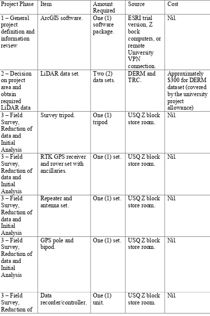
B.2 Resource Requirements ... 95
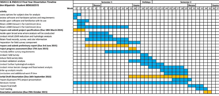
B.3 Project Timeline ... 97
Appendix C Risk Assessments ... 98
C.1 Risk Assessment for Project Success ... 98
C.2 Risk Assessment for Practical Project Activities ... 99
Appendix D Photos ... 103
D.1 Photos of East Creek ... 103
D.2 Photos of Field Survey ... 108
Appendix E Additional ArcMap Outputs ... 113
Appendix F Static Survey Data ... 123
F.1 Adjustment Report ... 123
List of Figures
Figure 2.1 Trimble AX80 airborne LiDAR system (Trimble AX80 Airborne LiDAR
Solution 2014) ... 7
Figure 2.2 Components of the Leica ALS80 airborne laser scanner (Leica ALS80 airborne laser scanners 2014) ... 8
Figure 2.3 Components of the Optech Galaxy (Optech Galaxy airborne LiDAR system 2015) ... 8
Figure 2.4 Scanning mechanisms from top left, clockwise: Oscillating Mirror, Palmer Scan, Fibre Scan, Rotating Polygon (Wehr & Lohr 1999) ... 9
Figure 2.5 Typical processing steps for laser scanner data (Wehr & Lohr 1999). ... 11
Figure 3.1 Toowoomba in South East Queensland (South East Queensland 2015) ... 23
Figure 3.2 1850 Map of Drayton Swamp - East and West Creeks can be recognised (Toowoomba 'where the water sits down' 2015) ... 23
Figure 3.3 Map of Toowoomba and creek systems (TRC 2015a) ... 25
Figure 3.4 Location of East Creek catchment in relation to the other branches of the Gowrie Creek catchment in the area of Toowoomba, Southeast Queensland (Liu, Zhang & McDougall 2011) ... 25
Figure 3.5 Extent of tiles used for East Creek catchment analysis (DNRM 2012) ... 27
Figure 3.6 Extent of tile data on satellite image (Google 2013) ... 28
Figure 3.7 Area for conventional ground survey on East Creek (Google 2013) ... 29
Figure 3.8 Extents of static network (Google 2013) ... 31
Figure 3.9 Static network in Toowoomba (Google 2013) ... 31
Figure 3.10 Adjustment network on the small study area for survey including RTK measurements (Google 2013) ... 32
Figure 3.11 Land cover types ... 34
Figure 3.12 Reduced detail survey data in ArcMap ... 36
Figure 3.13 High Flood Hazard Overlay used to generate flood level surface (TRC 2015b) ... 40
Figure 3.14 Conventional survey data with profile lines and TIN DEM used for flood surface delineation ... 41
Figure 3.15 Flood extents from 2010 LiDAR dataset ... 42
Figure 4.2 Hydrological node and link schema diagrams of East Creek catchment
generated from 2010 and 2012 LiDAR data... 48
Figure 4.3 Hydrological drain lines and catchments for East Creek derived from 2010 and 2012 LiDAR data using 25 000 m drain line catchment area threshold. ... 49
Figure 4.4 Variation in derived hydrological drain lines for 2010 (blue) and 2012 (orange) LiDAR raster DEMs – three areas of particular interest are noted ... 50
Figure 4.5 Variations of hydrologic outputs across area 1 (Google 2013) ... 51
Figure 4.6 Variations of hydrologic outputs across area 2 (Google 2013) ... 52
Figure 4.7 Variations of hydrologic outputs across area 3 (Google 2013) ... 52
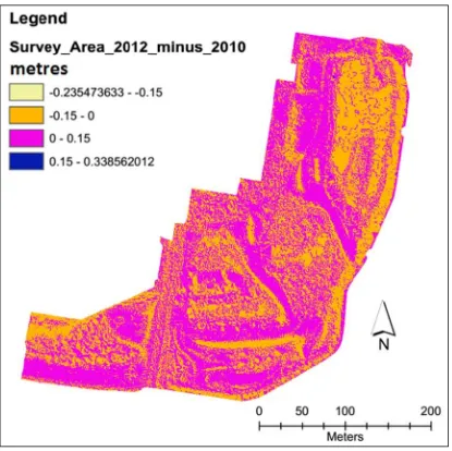
Figure 4.8 Difference raster generated by subtracting 2010 LiDAR data 5 m raster DEM from the 2012 LiDAR data 5 m raster DEM over the LiDAR data tiles covering East Creek catchment area of Toowoomba. Values are metres of difference. ... 55
Figure 4.9 Differences between 2010 and 2012 LiDAR raster DEMs for identified areas 1 and 2... 57
Figure 4.10 Differences between 2010 and 2012 LiDAR raster DEMs for identified areas 3 and 4... 57
Figure 4.11 Differences between 2010 and 2012 LiDAR raster DEMs for identified area 5 ... 58
Figure 4.12 TINs generated from 2010 and 2012 LiDAR and 2015 field survey datasets. ... 60
Figure 4.13 Distribution of sample points and land cover types over small subject area, note location of sample point effected by earthworks. ... 61
Figure 4.14 Histograms showing the distribution of errors between survey data and 2010 and 2012 LiDAR data TIN for the sample points lying within the Long Grass, Short Grass and Bitumen land cover types (See Appendix E for full size graphs). ... 65
Figure 4.15 Histograms showing the distribution of errors between survey data and 2010 and 2012 LiDAR data TINs for the sample points lying within Water Reeds and Trees land cover types and the total set of sample points (See Appendix E for full size graphs). ... 66
Figure 4.16 0.5 m resolution raster DEMs generated from datasets to the extents of the small survey area. ... 68
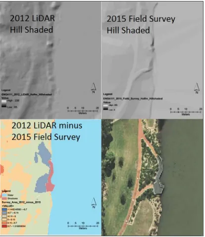
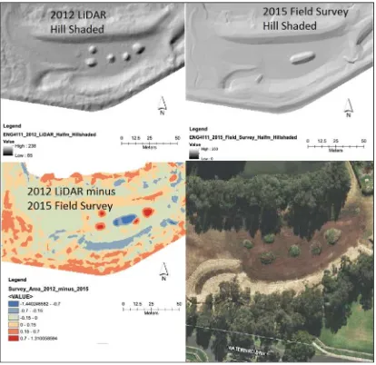
Figure 4.17 Difference raster generated by subtracting the conventional field survey 0.5 m resolution raster DEM from the 2010 LiDAR data 0.5 m resolution raster DEM. ... 69
Figure 4.18 Difference raster generated by subtracting the conventional field survey 0.5 m resolution raster DEM from the 2012 LiDAR data 0.5 m resolution raster DEM. ... 70
Figure 4.20 Difference raster generated by subtracting the 2010 LiDAR data raster from
the 2012 LiDAR data raster, created using different colour symbology ... 72
Figure 4.21 Google Earth satellite images over and around the bicentennial waterbird habitat showing changes over time (Google 2013). ... 75
Figure 4.22 Areas, in the area covered by conventional survey, with excessive residuals show potential instances of terrain change. This difference raster is the same as Fig. 4.18 (2012 LiDAR raster DEM minus conventional field survey raster DEM). ... 76
Figure 4.23 Potential terrain changes on northern side of lake on northern side of 9.2 ha surveyed area (TRC 2015b). ... 77
Figure 4.24 Potential terrain changes on western side of lake on northern side of 9.2 ha surveyed area (TRC 2015b) ... 78
Figure 4.25 Potential terrain changes on western side on south eastern side of 9.2 ha surveyed area (TRC 2015b) ... 79
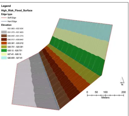
Figure 4.26 Flood surface TIN created from the four cross sections. ... 81
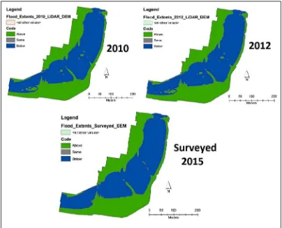
Figure 4.27 Flood surface extents applied to the three TIN DEMs over the 9.2 ha study area ... 82
Figure B.1 Dissertation planning schedule ... 97
Figure D.1 Facing southwest from Mackenzie Street upstream along East Creek ... 103
Figure D.2 Facing northeast into Bicentennial Waterbird Habitat ... 103
Figure D.3 Facing northwest towards Mackenzie Street form Bicentennial Waterbird Habitat... 104
Figure D.4 Facing south in the Toowoomba Bicentennial Waterbird Habitat ... 104
Figure D.5 Facing east over lake in Bicentennial Waterbird Habitat ... 105
Figure D.6 Facing north over lake in Bicentennial Waterbird Habitat onto Alderley St ... 105
Figure D.7 Tree cover beside water on eastern side of field surveyed area ... 106
Figure D.8 Facing west across Garnett Lehmann Park detention basin ... 106
Figure D.9 Facing north downstream from Garnett Lehmann Park detention basin .... 107
Figure D.10 Trimble R8 receiver set up over PSM 178770 at Horner’s Reserve in Centenary Heights for static observations ... 108
Figure D.11 Receiver setup over PSM 178772 to log data for static survey ... 108
Figure D. 12 Antenna height measurement - here measurements were made to centre of bumper (the black line around the middle of the receiver) ... 109
Figure D.13 Trimble R8 RTK GNSS equipment used to take RTK control observations on control marks within the survey site ... 109
Figure D.15 Trimble S6 robotic total station set up beside culvert in Bicentennial
Waterbird Habitat ... 110
Figure D.16 Facing east from target set up backsight to Trimble S6 Robotic Total Station in the background ... 111
Figure D.17 Besides back site setup on station 104 facing south ... 111
Figure D. 18 Surveying Swamp Area in Bicentennial Waterbird Habitat ... 112
Figure E. 1 Longitudinal profile of East Creek (Liu, Zhang & McDougall 2011) ... 113
Figure E. 2 Profiles of longest flow lines (LFL) based upon 2010 and 2012 LiDAR 5 m raster DEMs for East Creek ... 114
Figure E.3 Histogram showing the distribution of residuals when comparing 2010 LiDAR data TIN to conventional field survey sample points over entire area ... 115
Figure E.4 Histogram showing the distribution of residuals when comparing 2010 LiDAR data TIN to conventional field survey sample points over bitumen and concrete. ... 115
Figure E. 5 Histogram showing the distribution of residuals when comparing 2010 LiDAR data TIN to conventional field survey sample points over short grass. .. 116
Figure E. 6 Histogram showing the distribution of residuals when comparing 2010 LiDAR data TIN to conventional field survey sample points over long grass and shrubs. ... 116
Figure E. 7 Histogram showing the distribution of residuals when comparing 2010 LiDAR data TIN to conventional field survey sample points over trees. ... 117
Figure E. 8 Histogram showing the distribution of residuals when comparing 2010 LiDAR data TIN to conventional field survey sample points over water reeds. . 117
Figure E. 9 Histogram showing the distribution of residuals when comparing 2012 LiDAR data TIN to conventional field survey sample points over entire area. .. 118
Figure E. 10 Histogram showing the distribution of residuals when comparing 2012 LiDAR data TIN to conventional field survey sample points over bitumen and concrete ... 118
Figure E. 11 Histogram showing the distribution of residuals when comparing 2012 LiDAR data TIN to conventional field survey sample points over short grass. .. 119
Figure E. 12 Histogram showing the distribution of residuals when comparing 2012 LiDAR data TIN to conventional field survey sample points over long grass and shrubs. ... 119
Figure E. 13 Histogram showing the distribution of residuals when comparing 2012 LiDAR data TIN to conventional field survey sample points over trees. ... 120
Figure E. 14 Histogram showing the distribution of residuals when comparing 2012 LiDAR data TIN to conventional field survey sample points over water reeds. . 120
List of Tables
Table 3.1 LiDAR metadata for 2010 LiDAR dataset collected by Schlencker Mapping Pty Ltd (Schlencker Mapping, cited in Burke, 2013, p.17) ... 26 Table 3.2 Results from adjustment of control marks in TBC ... 33 Table 4.1 Hydrologic analysis results of East Creek based upon 5 m resolution raster DEMs which were generated from 2010 and 2012 LiDAR data... 45 Table 4.2 Statistics of the difference raster generated by subtracting 2010 LiDAR data 5 m raster DEM from the 2012 LiDAR data 5 m raster DEM ... 56 Table 4.3 2010 LiDAR data compared against field survey by comparing interpolated Z values of 2010 LiDAR data TIN with field survey sample point Z values ... 61 Table 4.4 2012 LiDAR data compared against field survey by comparing interpolated Z values of 2012 LiDAR data TIN with field survey sample point Z values ... 62 Table 4.5 Effect of earthworks changes on error statistics. ... 64 Table 4.6 Statistics from 0.5 m resolution difference raster - 0.5 m resolution DEM from 2010 LiDAR data minus 0.5 m resolution raster DEM from conventional field survey data raster. ... 73 Table 4.7 Statistics from the 0.5 m resolution difference raster - 0.5 m resolution DEM from 2012 LiDAR data minus 0.5 m resolution raster DEM from conventional field survey data raster. ... 73 Table 4.8 Statistics from the 0.5 m resolution difference raster – 0.5 m resolution DEM
Chapter One - Introduction
1.1
Background
The reported number of disastrous floods and storms has tripled over the last three decades (Klemas 2015). It is considered that even small changes in climate conditions can lead to large increases in flood magnitude (Knox 1993). Floods can destroy buildings, roads and bridges, rip out trees, devastate agricultural crops, cause mud slides and threaten human lives. In fact, in the United States, floods kill more people than any other weather – related disaster events (Klemas 2015).
In late 2007, major floods struck western, central and eastern Africa. 1.5 million people were affected in 18 countries, hundreds of thousands were displaced and nearly 300 people were killed (Smith 2007). In 2008 flooding in northern India effected 394 square miles and 2.1 million people, and killed more than 2 000 (Timmons & Kumar 2008). A major flood event struck China in summer 2010 where 230 million people were affected in ten provinces with 4 300 dead or missing and 15 million people were evacuated. Twenty-five rivers set record high levels (Hays 2013). Whilst many other major floods of a large scale have occurred across the globe over the last decade, this gives an indication of the challenges faced by both peoples and governments in coping with these events.
The flooding in Queensland from December 2010 to January 2011 is of particular significance for this dissertation. This began with significant rains in September 2010. Cyclone Tasha crossed the far North Queensland coast on December 24 2010 bringing heavy and substantial rainfall. 200 000 people were affected by this event state-wide with an estimated economic loss of $2.38 billion and 35 confirmed deaths.
The flash flooding in Toowoomba on January 10 2011 is directly related to this dissertation and provides a detailed example of major flash flooding. The Bureau of Meteorology (BOM) record station in Middle Ridge, Toowoomba, recorded a total of 452.6 mm for December 2010. In January 2011, 140.2 mm was recorded leading up to January 10, with a total for the month of 434.6 mm (BOM 2011).
between 1:30 pm and 2:15 pm (The nature and causes of flooding in Toowoomba 10
January 2011 2011)
Flood level data was recorded by the Cranley stream gauge which is on Gowrie Creek, several kilometres downstream of the junction between East and West Creeks. The peak according to the gauge was 3.67 m. However there is a suspected malfunction in the erratic trace of flood gauge levels from 2:00 pm – 4:00 pm that day. The flooding between 1:30 pm and 2:45 pm was rated as severe flash flooding and in some areas, the flooding exceeded the Q100 for the catchments (The nature and causes of flooding in Toowoomba
10 January 2011 2011), which is the instantaneous flow from a particular watershed that
would only be exceeded every 100 years on average (Tolland, Cathcart & Russell 1998). The bridges lower down along the catchments of East, West and Gowrie Creeks were inundated and damaged. The rapidness of the flooding caught motorists off guard and consequently cars were stranded or swept away, some getting “wrapped” around bridge pillars by the supreme force of the floodwaters. A woman and her teenage son lost their lives in the event.
In the aftermath of such floods, authorities have a significant task in responding to the damage and undertaking future mitigation activities. After the December 2010 and January 2011 Queensland Floods, the Queensland Government set up the Queensland Floods Commission of Inquiry (QFCI) to investigate the sequence of events and an interim report (Interim Report 2011) and final report (Final Report 2012) were prepared. This also covered future flood mapping and mitigation.
1.2
Aim and Objectives
The aim of this research project is to use LiDAR data to perform hydrologic analysis of a catchment area and to assess the usefulness and reliability of LiDAR data for hydrologic analysis and other related applications.
To achieve this aim, the following objectives have been set for this project:
Review existing literature on airborne LiDAR data and its application to hydrologic and hydraulic modelling
Obtain LiDAR data for a suitable catchment area
Undertake a conventional field survey of a small portion of this catchment area to validate the LiDAR data.
Prepare hydrologic models of the catchment area based on the LiDAR data
Model the comparison of conventional field survey data with LiDAR data
Use data comparison analysis to detect terrain changes
Model flood extents for a flood surface using the field survey and LiDAR data
Based upon results of the above tasks, assess the reliability and usefulness of LiDAR data for these tasks.
Make recommendations for further research to enhance the progress of these findings and to subsequently develop the future use of LiDAR data for hydrologic and hydraulic applications.
1.3
Expected Benefits
1.4
Dissertation Outline
This dissertation contains five main chapters.
Chapter One - Introductionprovides the background for this research project. The aims and objectives for the project are listed and the expected benefits are summarised. The structure and content of this dissertation is outlined.
In Chapter Two - Literature Review, the current literature and other appropriate works in the field are reviewed to establish the current progress in the field and determine particular areas of interest.
Chapter Three - Methodology describes the scope and areas of analysis, data acquisition, modelling of data and analysis that was applied.
Chapter Four – Results and Discussion provides a detailed report on the analysis conducted including hydrologic, error, terrain change and flood extent analysis.
Chapter Two - Literature Review
2.1
Introduction
In this chapter, the existing literature related to several relevant topics is outlined. Firstly literature related to the history of the development of airborne LiDAR and the current state of the technology is investigated. The available information on the components and principles of LiDAR systems is given. Past research on qualities of LiDAR data such as accuracy assessments, digital elevation model (DEM) interpolation and filtering is summarised. Past investigations of effectiveness of LiDAR for hydrologic and hydraulic modelling are also noted.
2.2
History of Airborne LiDAR
The invention of LiDAR technology came after other technologies were developed that use similar principles but different physical phenomena like SONAR (sound navigation ranging (SONAR definition 2015) and RADAR. Bats (Chiropter) actually use a SONAR system to navigate through dark caves. The bat emits short loud chirps through its nose and receives the echo back through its ears to provide a three – dimensional view of its surroundings to avoid obstacles (A brief history of LiDAR 2015). RADAR technology was first utilised in technology by Christian Huelsmeyer’s “Telemobilescope”, which was a device mounted onto ships which would warn operators when other ships (large metal objects) were detected at up to three kilometres away.
to today’s systems, but the advancements confirmed the growing belief in LiDAR as a new spatial data capture technique.
In the early 2000s, there was significant development in Computer Aided Drafting (CAD) and Geographic Information Systems (GIS) to better handle huge LiDAR datasets. Further developments included reliable POS systems (Inertial Navigation System (INS) or Inertial Measurement Unit (IMU) and GPS (Global Positioning System) combined), more stable hardware systems, and the ability to capture return intensities, LiDAR specific software and robust IT infrastructure. Scanners of 50 000 points per second were developed, niche market LiDAR services were provided to industry and government entities began to develop standards for quality assurance and accuracy reporting of LiDAR surveys. Current systems are capable of measuring beyond 250 000 points per second, emitting multiple pulses and gathering multiple returns (Geog 481 topographic
mapping with LiDAR 2014)
2.3
Current LiDAR Systems
For the purpose of reviewing current status of LiDAR technology, three LiDAR systems from different manufacturers are detailed below.
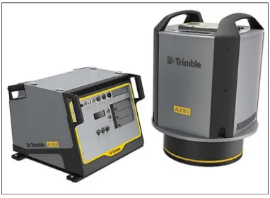
2.3.1 Trimble AX80
Figure 2. 1 Trimble AX80 airborne LiDAR system (Trimble AX80 Airborne LiDAR Solution 2014)
2.3.2 Leica ALS80
The Leica ALS80 airborne laser scanner (Fig. 2.2) has a 1.0 MHz PRF. It can be used at heights up to 5 000 m above ground level. It has three user selectable scan patterns, point density multiplier technology and also has integrated flight management software (Leica
Figure 2. 2 Components of the Leica ALS80 airborne laser scanner (Leica ALS80 airborne laser
scanners 2014)
2.3.3 Optech Galaxy
The Optech Galaxy laser scanner (Fig. 2.3) has a 550 kHz PRF and can receive eight returns per emitted pulse. It can be used at heights of up to 4 500 m above ground level. It also has integrated flight management software. Specification also give an approximate expected vertical accuracy of 0.2 m (Optech Galaxy airborne LiDAR system 2015).
2.4
Components and Principles of LiDAR Systems
Whilst LiDAR systems vary according to manufacturer and the finer details of the workings are classified for competitive reasons, they all consist of the same fundamental components.
2.4.1 Laser Scanner
The laser scanner is made up of two items: a ranging unit and an opto – mechanical scanner. A ranging unit measures either via pulse return time directly or indirectly through phase difference. The pulse method is most popular. An opto–mechanical scanner performs the scanning required to capture the numerous points required. There are various system types, including oscillating mirror, palmer scan, fibre scan and rotating polygon scan (Wehr & Lohr 1999). Fig. 2.4 illustrates these different scanning techniques.
Figure 2. 4 Scanning mechanisms from top left, clockwise: Oscillating Mirror, Palmer Scan, Fibre Scan,
With regards to scanning parameters, swath width refers to the width of a complete scan as the sensor moves along its path, field of view (FOV) is the width area in which the scanner’s sensor can pick up the return signal and instantaneous field of view (IFOV) is the narrow divergence of the laser beam itself as it leaves its source and reflects back from a surface (Wehr & Lohr 1999).
2.4.2 GPS System
A GPS unit forms part of the POS which provides required information to calculate the real world coordinates for the LiDAR data. A survey – grade receiver is required, probably with dual frequency capability for improved location fixing. Corrections to the GPS measurements are required and would probably be applied using Real Time Kinetic (RTK) or post processing techniques. The sensor would usually be operated within 50 miles (80 km) of the base station to achieve suitable GPS accuracy. Initialisation is usually carried out before and after flights to check the satellite fix. GPS positions are usually recorded at 0.5 – 1 sec intervals to correct the IMU measurements and can usually achieve accuracies of 30 – 40 mm (Wehr & Lohr 1999).
2.4.3 Inertial Measurement Unit
The POS system has an IMU (or INS) to calculate inclination angles of the unit and to determine position continuously between the GPS positions. INS includes three inertial gyroscopes mounted on the laser sensor to measure angular rotations. Accelerometers are utilised to measure the speed and direction of the LiDAR sensor. The INS system is updated by the GPS positions every 0.5 – 1 second.
2.4.4 Derivation of Point Data
Particular calibration techniques vary according to manufacturer and are usually kept confidential (Wehr & Lohr 1999). Fig. 2.5 illustrates the processing of LiDAR data.
2.5
LiDAR Data and DEM
2.5.1 LiDAR Data File Formats
In the past, the two main LiDAR data file formats were American Standard Code for Information Exchange (ASCII) and proprietary formats. As the LiDAR technology and market developed, problems and limitations with these file formats were highlighted. The ASCII file format had limited performance as they contained large amounts of data even for relatively small files and interpretation of them by software was slower. Specific LiDAR information is also lost in this format. Propriety systems had the problem of data from one system not being compatible with another. To overcome these problems a LAS 1.0 file format was released by American Society for Photogrammetry and Remote Sensing (ASPRS) in 2003. The current LAS file format is LAS 1.4 which was released in 2011. The LAS file was designed to be a public file format that can be used for all systems. It is a binary file format and it can maintain information specific to LiDAR without becoming overly complex. It also the ability for customization by the LiDAR mapping community (ASPRS 2015).
2.5.2 LiDAR Data Accuracy
Besides the internal errors of LiDAR systems, data accuracy is also effected by external factors – flying height, terrain variation, terrain cover (e.g. vegetation type), sampling angle and spatial resolution (Casas et al. 2006).
Bowen and Waltermire (2002) validated LiDAR data by using RTK GPS to measure points which matched horizontal position of LiDAR points and also by performing cross sections over the survey area. It was found that published LiDAR accuracies were only achievable on no more than moderately smooth and flat ground with errors of 1 – 2 m occurring on terrain with significant relief which would have been caused by the implication of the horizontal inaccuracies. It was also found that definition of linear features was limited according to the point resolution (usually 1 – 5 m).
In another study, DEMs were derived from airborne laser scanning (ALS), photogrammetry and space-borne radar interferometry. RTK GPS equipment was mounted on a vehicle and used to collect profile data along roads for validation. Comparisons between the collected profiles and the DEMs resulted in 0.15 – 0.3 m RMSE for ALS, 1.03 – 3.75 m RMSE for photogrammetry and 4.26 – 27.81 m RMSE for InSAR DEM (Hsing-Chung et al. 2004).
Casas et al. (2006) found that LiDAR performed poorly in measuring submersed surfaces accurately. Hydrographic survey was carried out over the subject area and the LiDAR data had an RMSE of 1.603 m for submersed terrain as opposed to 0.302 m for non-submersed terrain.
According to Su (2006) slope gradient had an increasing effect upon errors. Elevation was overestimated in forests but underestimated in meadows. LiDAR sampling distance was considered a less important factor in accuracy.
Another study, over the catchment of the Koondrook-Perricoota Forest, NSW, a section of flood plain forest, reported errors significantly greater than specified, with an average error of between 0.126 m - 0.338 m. However the 736 points that were collected with RTK GPS only represented a small area of the total LiDAR dataset. Also a vertical accuracy of 1 mm was stated for the validation points - this would be very difficult to achieve with RTK GPS (Vaze & Teng 2007).
2.5.3 Approaches to LiDAR Data Validation
Techniques of validating LiDAR data have already been briefly mentioned. Time and resource efficient ways of checking the accuracy of LiDAR have been sought. Liu (2011) prescribed a technique of testing accuracy by utilising existing permanent survey marks or new control points and checking the accuracy by the nearest point technique or interpolation. This technique was utilised by Thompson and Croke (2013) where pre- and post-flood (January 2011 floods) LiDAR dataset was used to analyse hydraulics and erosion of the flood event. DEM uncertainty of the post flood dataset was tested with survey marks from a state-wide dataset giving a mean height difference of 0.08 m and a standard deviation error (σ error) of 0.17 m.
2.5.4 DEM Interpolation
Liu (2009) performed validation and cross validation on Inverse Distance Weighting (IDW), Kriging and Local Polynomial Interpolation algorithms and recommended the IDW technique as a trade-off between accuracy and computing time when applied to LiDAR data.
2.5.5 DEM Filtering to Remove Non-Ground Points
A useful concept is the multiple returns from a single LiDAR pulse as occurs in forested areas. The laser pulse strikes a target that does not completely block its path and the remainder continues to a lower object. Algorithms can be used remove the non-ground data or the non – ground data can be used to measure tree heights (Liu 2011).
errors occurred in a few instances and the development of a future human interaction filter was suggested.
A study examined the performance of filtered LiDAR data over forested gulleys on a southeast piedmont of USA. Ground survey via RTK GPS and levelling was used for validation. It was found that performance was good at a broader scale but only gulleys with a top width of 3 m or greater were properly mapped. LiDAR tended to underestimate depth and overestimate width of gulleys. Poor bare earth data densities, shadowing of gullies and filtered topography discount were considered to have caused this (James, Watson & Hansen 2007).
With thick vegetation, filter algorithms do not always produce sufficiently accurate results for finer applications. Hladik and Alber (2012) carried out a study over a coastal salt marsh and applied species specific correction factors for 10 classes of vegetation cover and was able to improve the SDE from 0.10 m +/- 0.12 m to -0.01 m +/- 0.09 m. The improved accuracy made the data useable in salt marsh study applications where accuracy is important where low lying areas are involved and small elevation differences have major effects on analysis.
2.6
Application of LiDAR Systems.
2.6.1 LiDAR for Hydrologic Modelling
For hydrologic modelling applications, a DEM with accuracies of less than 0.5 m is recommended while the accuracy requirements for water management plans and sub catchment delineation is stated as 0.5 – 1 m (McDougall 2008). Standard LiDAR accuracies have found to be well within this tolerance most of the time as shown in the previous section (refer 2.5.1).
2.6.1.1 Effects of LiDAR DEM Resolution and Accuracy on Hydrologic Modelling
Zhao et al. (2010) investigated effects of DEM accuracy upon hydrological parameters and found that at the watershed scale, DEM resolution mainly determined accuracy of areas and boundaries of sub-basins and the distribution of flow lines while elevation differences was more effected by actual DEM accuracy. The average length of stream lines per hectare was found to be sensitive to both accuracy and resolution. Overall DEM resolution was found to dominate the quality of hydrologic parameters derived at the sub – basin scale.
A study by Harris (2013) used a 10 m resolution LiDAR DEM generated in 2012 over Ipswich City Council (ICC) was compared to a 20 m resolution DEM generated from 5 m contours in 2004. The hydrological analysis on the 2012 LiDAR DEM resulted in a 20% increase in waterway lengths which could affect calculated remediation costs and water quality modelling. A stream definition threshold area of 0.1 km2 produced a total stream length of 10.88 km while 0.025 km2 produced 19.35 km of streams.
value of less than 1% of maximum flow accumulation while 1% was appropriate for low drainage density areas.
2.6.1.2 LiDAR DEM Difficulties and Solutions in Hydrologic Modelling
A potential issue with LiDAR data, raised by Harris (2013), is a lack of knowledge of the subject terrain in situations where LiDAR data is collected over large areas. Pits in a DEM cause a disconnected drainage network and therefore have to be filled, however, large amounts of filling can cause incorrect drainage representation and negate the benefits of high resolution data. An example of this was a bridge where standard fill function yielded inaccurate delineation of the real waterway path and regarding this it was concluded that either the DEMs or the waterway networks would have to be manually edited in such circumstances.
Jones et al. (2008) detailed a useful hydrological analysis technique for low relief landscapes (where hydrological analysis is difficult) that uses high resolution LiDAR data to divide the subject area into numerous small “hydrological facets” and aggregates these into larger facets to generate a link – node drainage flow network successfully.
2.6.2 LiDAR for Hydraulic Modelling
2.6.2.1 Hydraulic Modelling
Rigby (2006) states that hydraulic modelling techniques should be seen as just a means to an end. Models should be selected according to their ability to simulate the flood event accurately and the required outputs from the models. Therefore there is a need for understanding flood behaviour and the limitations of various models.
Hydraulic models vary according to the behaviour of the flood flow being modelled. 1D modelling is where flood flow is parallel to a stream channel. Quasi 2D models are similar except they can model several stream branches. Examples of these types of models include Estry, HEC-RAS, MIKE11 and XPFLOOD. 2D models simulate flood behaviour which flows across a surface with little correlation to the main stream channel. Examples of 2D models are FLO2DH, Mike 21 and Tuflow. 3D models simulate hydraulic flow where velocity varies significantly with depth such as in lakes. However high complexity of 3D models means excessive computational costs. Additional models that are used internationally include TELEMAC – 2D, INFOWORKS, WATFLOOD, FLO2D and SOBEK (Rigby 2006).
Typical outputs of hydraulic models include flood water surface elevation, depth, velocity, hydraulic hazard classification and flood risk classification. Models can provide these outputs in a static (at a single point in time) or dynamic (at different times) format (Rigby 2006).
The most immediate use of flood modelling data is to inform emergency response mechanisms in flood events. However there are a variety of different flood maps that indicate different aspects of flooding effects. Flood hazard maps consider the intensity of the flood situation and associated exceedance probability to derive flooding hazards. Flood vulnerability maps consider exposure and susceptibility to calculate flood vulnerability and flood risk mapping provides the spatial distribution of the risk (Begum, Stive & Hall 2007).
Dottori, Di Baldassarre and Todini (2013) pointed out that the accuracy of results is not necessarily increased by higher resolution data and modellers should focus on the purpose of the model (Begum, Stive & Hall 2007), that is, reliable flood mapping. Too much detail can be misleading with regards to output model accuracy and can complicate the process unnecessarily.
2.6.2.2 Developments in Applying LIDAR to Hydraulic Modelling
Hollaus, Wagner and Kraus (2005) identified the potential of LiDAR data for hydraulic modelling, noting the high level of automation and the ability to use the same data for different applications. Whilst limitation were found in the measurement of vegetation height on areas of tall grass and scrub, these difficulties were hoped to be overcome by future systems able to record full echo – waveforms (which have since been developed as found above). Airborne LiDAR data combined with colour infrared (CIR) imagery had noted potential for object oriented land cover classification which could be applied for hydrologic and hydraulic modelling. Likewise Mason et al. (2007) detailed a method of deriving hydrologic models using LiDAR DEM and digital map data to extract various manmade and non-manmade features and derive friction parameters for modelling. New ways of capturing peak levels have been investigated. In one study on the January 2011 flood event in Brisbane, photos captured privately (that satisfied certain criteria to correctly depict peak flood levels) were obtained through social media websites and used to identify flood level markers, which were subsequently surveyed via RTK GPS (total station was used where satellite fix was unachievable) and successfully used to model the flood event (McDougall 2012).
impractical for traditional planform or cross – sectional surveys), it could provide a sophisticated system for landscape change assessment.
2.6.2.3 LiDAR DEM Resolution, Accuracy and Hydraulic Modelling Performance
Haile and Rientjes (2005) experimented on a 1.5 m resolution LiDAR DEM over the city of Tegucigalpa in Honduras. The 1.5 m resolution DEM was resampled to resolutions of up to 15 m. Features smaller than the resampled grid size were eliminated, and flood extent, flow velocity and depth were effected. All these factors are interrelated and it was difficult to explain precisely. It was concluded that low resolution DEMs don’t explicitly simulate topographic features. This is considered acceptable in topographically simple rural areas but river banks, dykes, roads and buildings all have significant effect on models and must be mapped to sufficient accuracy. There the simulation of topography was considered to have significant effects on flood simulation results.
Small terrain features can have a large effect on flood flow. Néelz et al. (2006) observed that the gridded nature of LiDAR data and DEMs results in larger errors on steep slopes, embankments and any terrain features of small dimension compared to DEM grid size. Casas et al. (2006), in a study of a 2 km reach of the Ter River in Spain, obtained a RMSE of 4.5 m for 1:5 000 contour map data and a 0.3 m RMSE of water surface elevation when compared to an RTK GPS – based DEM. It was generally found that decreases in resolution caused increases in water level.
Schumann et al. (2008) compared water level stages from flood models derived from a 2 m resolution LiDAR DEM, a 50 m resolution vectorised contour DEM and a three second geographic resolution Shuttle Radar Topographic Mission (SRTM) DEM over Alzette River north of Luxembourg City in Luxembourg. Water stage RMSE were 0.35 m, 0.7 m and 1.07 m for LiDAR, contour and SRTM DEMs respectively.
2.7
Conclusion
This literature review has covered the use of LiDAR with a focus on hydrologic and hydraulic modelling. The history of the development of LiDAR has been outlined and examples of current airborne LiDAR technologies are given. The principles and components behind LiDAR systems have been covered. Past research regarding LiDAR accuracy was reviewed. DEM generation techniques were touched upon. Airborne LiDAR data applied to hydrologic and hydraulic modelling was also reviewed.
Chapter Three - Methodology
3.1
Introduction
This chapter describes the methodology used to achieve the project outcomes. The history and details of East Creek are outlined. Acquisition of LiDAR and field survey data for this project is explained. The approach to the conventional ground survey for validation and techniques are described. The techniques and software tools used for hydrologic analysis are detailed. The techniques used to compare the LiDAR data and conventional ground survey data are outlined, including how this is used for terrain analysis. Flood zone delineation strategies are also explained.
3.2
Study Area - East Creek in Toowoomba
The East Creek catchment in Toowoomba has been selected as the subject area for the hydrologic modelling and analysis for this dissertation, as suitable LiDAR datasets covering the area are available and East Creek also played an important part in the January 10 2011 floods in Toowoomba. The history of the development Toowoomba, and particularly of the creek networks in Toowoomba, shows factors which have influenced the severity of the January 10 2011 flood events in Toowoomba. A basic outline of Toowoomba’s history is of relevance in this dissertation.
Figure 3. 1 Toowoomba in South East Queensland (South East Queensland 2015)
Figure 3. 2 1850 Map of Drayton Swamp - East and West Creeks can be recognised (Toowoomba 'where
Toowoomba sits in two catchment areas: the eastern area which flows into south east Queensland and the western area which consists of most of Toowoomba city and flows into the Murray Darling Basin (Toowoomba waterways and catchments 2012). The western area contains the catchments of East, West and Black creeks which drain into Gowrie Creek (Figs. 3.3, 3.4). East and West creeks have a catchment area of 15.59 km2 and 15.87 km2 respectively. They are both characterised by moderately steep side slopes. The upper sections are steeper with impervious drain surfaces which accelerate runoff (Liu, Zhang & McDougall 2011).
Due to the channel characteristics and the need to manage flooding issues, these catchments are covered by the Gowrie Creek catchment management strategy which was first prepared in 1998. A major part of this plan was the construction of detention basins (artificial alterations to terrain along a water course which serve to store flood water run-off and release it through outlet structure to reduce peak flows downstream (East Creek
detention basins 2015)) on East and West Creeks. The original proposed number of 22
Figure 3. 3 Map of Toowoomba and creek systems (TRC 2015a)
Figure 3. 4 Location of East Creek catchment in relation to the other branches of the Gowrie Creek
3.3
Data Acquisition
3.3.1 LiDAR Datasets
It was considered beneficial to obtain LiDAR data from before and after floods of January 10 2011 as this would allow any significant effects of the flood to be identified. LiDAR datasets from 2010 and 2012 were obtained to provide the temporal variation desired. The 2010 dataset was captured by Schlencker Mapping Pty Ltd for Toowoomba Regional Council. It was captured from June 29 - July 16 2010. The ASCII “.txt” format file tiles of 1 km × 1 km were utilised and 32 of such tiles were required to cover the entire East Creek catchment (Figs. 3.5, 3.6).
Table 3. 1 LiDAR metadata for 2010 LiDAR data set collected by Schlencker Mapping Pty Ltd
(Schlencker Mapping, cited in Burke, 2013, p.17)
Acquisition Start Date June 29 2010
Acquisition End Date July 16 2010
Device Name Optech ‘ALTM Gemini’
IMU Applanix ‘Litton 510’
Flying Height (AGL) 1 200m
No. of Runs 242
Swath Width 1 000m
Side Overlap 30%
Horizontal Datum GDA94
Vertical Datum AHD
Map Projection MGA Zone 56
Control 302 surveyed GPS control points
Vertical Accuracy +/- 0.15 m @ 1σ
Horizontal Accuracy +/- 0.22 m @ 1σ
Surface Type Ground and DTM
Average Point Separation 1.0 m
The 2012 LiDAR dataset was available and utilised in 1 km x 1 km tile ASCII “.txt” format as 1 m grid data and the required coverage was available. However limited metadata was available for this dataset over this area.
Figure 3. 6 Extent of tile data on satellite image (Google 2013)
3.3.2 Conventional Field Survey for LiDAR Data Validation
Robotic total station was the primary survey instrument used for the surface topography survey as the area contained a large number of trees and obstructions which would block satellite signals or cause multipath and it would take extra time to obtain a fixed position with GPS. The downside with total station survey is that it is more labour intensive, requiring more setup time, more human input and therefore more potential for operator errors. It is also limited to line of sight, which was limited at a number of survey station locations. These challenges were overcome by adding strategically placed setups and more work and highly accurate data was collected with which to validate the LiDAR data. A convention field survey was done covering 9.2 ha along East Creek, within LiDAR coverage, to create an independent dataset to check the accuracy and relevance of the LiDAR data. The 9.2 ha area surveyed covered the parkland along East Creek from the northern end of Ballin Drive Park (in line with Marguerita Court) to the northern edge of the Bicentennial Waterbird Habitat (refer Fig. 3.7).
trees. The area contains a numerous undulations, mounds, changes of grade and banks. Due to these site characteristics, less survey coverage was achievable in the given time than what would have been achievable in more even and flat terrain but the presence of the variety of features made the area very good for a more rigorous assessment of the capabilities and limitations of airborne LiDAR for measuring varying land cover types and acute topographic relief. This area was also chosen because it was easily accessible and was wide enough to contain flood extents for basic flood surface extent models (Fig. 4.27).
3.3.2.1 Preparation
The survey was planned out in ahead of time and requirements, such as survey equipment for sufficient time, existing coordinated Permanent Survey Marks (PSM) and site control marks, were managed.
Permanent Survey Mark (PSM) information public available via Queensland Globe was utilised. Queensland Globe is an overlay to Google Earth which provides an extensive variety of geographic information across Queensland. PSM mark locations and information are available via the Queensland Globe extension to Google Earth and this was used to determine existing control. PSM metadata freely available through Queensland Globe was utilised to locate PSMs in the field. Survey equipment and required supplies were sourced from the University of Southern Queensland (USQ) survey supply store. Prior to survey, survey pegs were placed for control marks in strategic locations around the site to maximise the efficiency and accuracy of the conventional field survey.
3.3.2.2 Control Data Collection
The conventional field survey was done between June 29 and July 8 2015. Due to the lack of coordinated PSMs close to the small study area it was considered necessary to perform static survey to give coordinates for PSMs in the vicinity and to connect to the same control marks and datum as the LiDAR datasets. Therefore a static survey was planned and logged data covering the static survey period was requested from major permanent reference stations around southeast Queensland (Fig. 3.8), including in Toowoomba (PSM 753327), Dalby (PSM 753334), Warwick (PSM 753333) and Gatton (PSM 753323).
Figure 3. 8 Extents of static network (Google 2013)
With the static control network confirmed, RTK control measurements were taken to the six survey peg control marks within the selected area on 1st July. Three minute observations were read to each of the marks from both PSM 118131 and PSM 97033 to achieve a dual occupation for each mark to provide redundancies (Fig. 3.10). The results are provided in table 3.2.
Figure 3. 10 Adjustment network on the small study area for survey including RTK measurements
Table 3. 2 Results from adjustment of control marks in TBC
Adjusted Grid Coordinates from RTK Survey
Point ID Easting (Metres) Easting Error (Metres) Northing (Metres) Northing Error (Metres) Elevation (Metres) Elevation Error (Meter) Constraint
100 398588.665 0.007 6947988.338 0.008 627.646 0.020 -
101 398551.824 0.008 6947855.469 0.008 629.163 0.021 -
102 398607.068 0.007 6947745.261 0.007 628.245 0.020 -
103 398475.977 0.006 6947758.837 0.006 629.972 0.019 -
104 398554.916 0.008 6947645.776 0.008 632.680 0.025 -
105 398375.248 0.008 6947678.499 0.010 631.252 0.024 -
118131 398678.026 (Fixed) 6948005.536 (Fixed) 626.803 (Fixed) ENe
97033 398300.866 (Fixed) 6947571.396 (Fixed) 634.427 (Fixed) ENe
3.3.2.3 DTM Survey
Using the control mark data provided, a Trimble S6 Robotic Vision Total Station together with a 360 degree Multi Track prism, TSC3 controller and other required ancillaries were utilised to carry out a full topographic survey of the narrow study area (9.2 ha). The survey was completed in 55 hrs from 1st July - 8th July with a total of approximately 6 250 points collected and an area of 92 490 m2 (9.2 ha) covered by the survey.
For the purpose of analysis, land cover types were classified as:
Bitumen and concrete
Short grass (mowed or up to 0.3 m high)
Long grass and shrubs (grass higher than 0.3 m and shrubs up to 2 m high)
Trees (5 – 30 m high)
Water (no hydrographic survey performed save spot heights below the water edge).
(Refer Fig. 3.11)
Figure 3. 11 Land cover types
Additional control marks were read to and occupied and resections were performed to allow line of sight to the entire area and therefore a complete survey dataset. In some instances reflector-less measurements were taken to ensure safety and reduce environmental impact. Island shorelines were also picked up this way to delineate location on the survey.
Vigilance was utilised to ensure the data was accurate. Pole heights were regularly checked my measuring a known mark before starting survey work. Instrument and backsight targets were measured accurately and checked. Stations were located to permit maximum inter-visibility to other marks and measurements were taken where extra control marks could be seen.
3.4
Hydrologic Analysis
A hydrologic analysis of East Creek catchment area was performed with the Arc Hydro 2.0 extension to ArcMap version 10.3 and done for both the 2010 and the 2012 LiDAR datasets separately. Firstly the .xyz ASCII tile files were converted into ArcMap feature classes. Then all of the feature classes were placed into a feature dataset. A terrain dataset was created and built from these feature classes in this feature dataset. A terrain to raster function was utilised to create 5 m resolution raster datasets covering the entire catchment area via the linear interpolation method.
3.5
LiDAR Data Validation
To test the accuracy of the LiDAR data, comparison tests were done. An overall assessment of accuracies was done by directly comparing the two raster DEMs upon which the hydrologic analysis was based. The 5 m resolution raster from the 2010 LiDAR data was subtracted from the 5 m resolution raster from the 2012 LiDAR data. This was done by performing this operation with the Raster Calculator tool in ArcMap. This provided a quick and simple test. However the conventional field survey data was to provide a more conclusive and detailed assessment of the LiDAR data accuracies.
3.5.1 Reduction of Conventional Field Survey Data
The data collected from the conventional field survey had to be reduced and processed to a suitable format to compare it with the LiDAR data. The conventional field survey data was downloaded and reduced with TBC software. The data was then exported into ESRI Shapefile format and imported into ArcMap 10.3. In ArcMap any additional reductions were completed (Fig. 3.12).
3.5.2 Modelling and Analysis
As the survey was mostly impractical for terrain under water and islands inaccessible by foot, analysis involving the survey data DEM was excluded from these areas. Buildings and structures were not included either.
A TIN of the reduced survey data was created in ArcMap. A portion of data covering the small study area was taken from both 2012 and 2010 datasets and a TIN DEM was created for each.
To check the accuracy of the LiDAR datasets, two methods were utilised:
Compare elevations at the surveyed points derived from each of the TIN DEMs
Compare raster DEMs derived from each of the datasets.
For the first technique, 200 sample points was taken from the conventional field survey data and elevations were interpolated from both the TIN DEM from 2010 LiDAR data and the TIN DEM from the 2012 LiDAR data using the Add Surface Information tool in ArcMap. Three separate feature classes containing sets of the 200 sample points (for each dataset) were used (one for the conventional field survey data elevations and the other two for the interpolated 2010 and 2012 LiDAR elevations). The attribute tables, for each of the three feature classes, were linked so that these elevation values could be compared statistically within the attribute tables. The survey data elevations were subtracted from the 2010 and 2012 datasets and the residuals were graphed on a histogram and statistically summarised. Sample points were also subdivided according to land cover type classification and statistics were generated in the same way for each land cover type classification.
The second technique was used mainly to check the statistics and graphs derived from the first technique and achieve complete coverage over the entire raster DEMs. A similar analysis was done but using raster DEMs instead. A 0.5 m resolution raster DEM was generated from each of the three TINs and raster data was clipped down to the survey area. The Raster Calculator tool in ArcMap was used to subtract raster cells values from one dataset by raster cell values for another dataset. Rasters were subtracted against each other to generate 0.5 m resolution raster difference DEMs:
Difference raster from conventional field survey data subtracted from raster DEM from 2012 LiDAR data
Difference raster from 2010 LiDAR data subtracted from raster DEM from 2012 LiDAR data
The 0.5 m resolution raster difference DEMs were also divided exclusively according to land cover classification polygons using the Clip function in ArcMap. Statistical summaries were recorded for each of the entire raster difference DEMs as well as the separate land cover types.
The first technique minimises generalisation error by providing direct interpolation between the points but is more appropriate for a small sample of survey points and is only as good as the selected sample data. The advantages of the second technique - using raster DEMs instead - is that less file space is required in the generation of them. ArcMap supports more functions with raster data. Instead of analysis being limited to the selected sample points, the analysis can cover the entire DEM. However each cell contains only a single elevation which has to be interpolate from a TIN or terrain dataset so there is more generalisation involved when using rasters and consequently more error introduced.
3.6
Flood Zone Delineation
Delineating flood extents is a secondary task for this project. Flood level delineation aids the understanding of the suitability and effectiveness of LiDAR data in determining flood extents and levels. The area of the conventional field survey was also used to do the flood surface delineation.
TRC surveyed the January 10 2011 floods extents (The nature and causes of flooding in
Toowoomba 10 January 2011 2011). However it found to be difficult to obtain this data
and then it may not cover required areas.
Bureau of Meteorology (BOM) rainfall records are available in several locations around Toowoomba including Middle Ridge and Toowoomba Airport. Data for the months of December 2010 and January 2011 have been obtained to illustrate the rainfall totals leading up to, during and after the event. This data was utilised to generate hydraulic models for West Creek by Topp (2014). However advanced hydraulic modelling using that data is beyond the scope of this dissertation.
Figure 3. 13 High Flood Hazard Overlay used to generate flood level surface (TRC 2015b)
Figure 3. 15 Flood extents from 2010 LiDAR dataset
3.7
Conclusions
The main objectives of this project are to perform hydrologic analysis on a catchment with LiDAR datasets, check the accuracy of this LiDAR data by performing a conventional ground survey and performing comparison analysis, check for temporal terrain changes between LiDAR datasets and model flood extents all for the purpose of assessing the utility of LiDAR data in the context of flood mitigation as well as land management, analysis and planning.
Analysis over the small study area involved comparing LiDAR datasets against each other and against the survey data with consideration of land cover. The High Flood Risk Zone overlay was modelled as a flood surface and the results with the different DEMs were analysed. Analysis over the large study area included hydrological modelling of East Creek’s drain lines, and complete catchment area and the comparison of the two LiDAR datasets over the large study area to determine the presence of any terrain changes or data characteristics.
Raster DEMs were created from the two sets of LiDAR data tiles covering East Creek catchment area. The two raster DEMs were compared to produce a difference raster. A separate hydrologic analysis was performed over the entire catchment of East Creek for each data set. To validate the quality of the LiDAR datasets, the field surveyed data was compared with the LiDAR data using raster and TIN DEMs. A basic terrain change analysis (between the points in time of the data capture) was done leading from these comparisons. A nominal flood surface was identified based upon flood risk overlay data published on council online mapping portals and modelled against the field survey and LiDAR datasets. In the next chapter the results of this project work will be detailed and discussed.
Chapter 4 - Results and Discussion
4.1
Introduction
In this chapter the results of the analysis as described in the previous chapter are explained, detailed and discussed. The results for the work covering the entire catchment area of East Creek are first discussed. This includes comparison of raster DEMs generated from the 2010 and 2012 LiDAR dataset, hydrological results based upon the raster DEMs and more detailed comparisons of stream lines and catchments extracted. In order to better understand the accuracy characteristics of the LiDAR datasets, DEMs generated from the LiDAR and field survey datasets over the 9.2 ha area covered by conventional field survey on East Creek are compared. Detailed statistics on these results are also given. Areas which experienced potential terrain changes are also analysed. Flood extents are delineated based upon available information and the three datasets over the small study area. From this detailed analysis the qualities and accuracies of LiDAR are better understood.
4.2
Hydrologic Analysis
As mentioned in the previous chapter, hydrologic analysis was done for the entire catchment of East Creek with a 5 m resolution raster DEM which was interpolated from the LiDAR data in ArcMap by averaging. The Arc Hydro extension of ArcMap was used to perform hydrologic analysis and all tools whose outputs were deemed relevant to the analysis, and applicable to the available datasets, were utilised.
Table 4. 1 Hydrologic analysis results of East Creek based upon 5 m resolution raster DEMs which were
generated from 2010 and 2012 LiDAR data
Value generated from 2010 LiDAR
Data
2012 LiDAR
Data
Results from
Liu, Zhang and
McDougall
(2011) Hydrologic Parameter
Watershed Area (m2) 14 920 800 15 613 225 15 590 000
Catchment Perimeter (m) 29 910 29 560 - Longest Flow Line - LFL (m) 8 813 8 697 -
RL Uppermost LFL 720.27 720.26 -
RL Pour Point LFL / East Creek 583.00 582.79 -
Height Difference -137.27 -137.47 -
Average Gradient 1:64 1:63 -
In table 4.1, the results from the two different datasets are compared. Watershed in ArcMap refers to the entire area flowing into a selected batch point raster cell. In this case it is the junction from East Creek to West Creek (hence the entire watershed area for East Creek catchment). The East Creek catchment area calculated from 2010 LiDAR data raster DEM is 692 425 m, 4.6% less than that calculated from 2012 LiDAR data raster DEM. However the catchment perimeter calculated from 2010 LiDAR data raster DEM is 350 m, or 1.2% longer, which suggests slightly more irregularity in the catchment boundary. The longest flow line (LFL) of the 2010 LiDAR dataset is 116 m (1.3%) longer.
These errors appear to be only at a small scale. It would be reasonable to attribute these to random errors in elevations, LiDAR data point distribution and generalisation errors from the creation of the raster. In this context it would be safe to say that no significant hydrological changes have occurred over the area at this scale between 2010 and 2012 and the variation provides a valuable indication of the reliability to be expected within the hydrologic analysis with this data. The areas of difference causing the variation of catchment area are shown in Fig. 4.5.
DEM Generation and Hydrologic Modelling Using LiDAR Data Glen Kilpatrick
DEM Generation and Hydrologic Modelling Using LiDAR Data Glen Kilpatrick
DEM Generation and Hydrologic Modelling Using LiDAR Data Glen Kilpatrick
4.2.1 Hydrologic Stream and Watershed Variation
As mentioned earlier in this chapter, variation in hydrologic outputs between LiDAR datasets captured at different points in time can give an indication of the reliability of those hydrologic outputs. Two major hydrologic output formats are drainage lines and watershed areas. It is of value to study the accuracy and reliability characte