Real-Time Load-Side Control of Electric Power Systems

(1)

Thesis by

Changhong Zhao

In Partial Fulfillment of the Requirements for the Degree of

Doctor of Philosophy

CALIFORNIA INSTITUTE OF TECHNOLOGY Pasadena, California

2016

(2)

Changhong Zhao

ORCID: 0000-0003-0539-8591

(3)

ACKNOWLEDGEMENTS

I owe my deepest gratitude to Professor Steven Low, for his generous support and helpful guidance during my PhD studies. Steven is a great scholar. He always keeps learning, and is enthusiastic to tackle challenging research problems that make real impacts. He is also the best advisor I could ever imagine. He understands what the students do from big picture to technical details, and is ready to provide advice whenever the students need. His professionalism and personality have set up a role model for me. I feel fortune to have worked with him.

I am grateful to my colleagues around the world, including Scott Backhaus, Janusz Bialek, Lijun Chen, Misha Chertkov, Florian Dörfler, Na Li, Feng Liu, Enrique Mallada, Kiyoshi Nakayama, Ufuk Topcu, and Yingjun Zhang, for our fruitful discussions and collaborations. Some of them indeed worked as my mentors at different stages of my research. I also want to thank the members of my candidacy and thesis committees: Professors K. Mani Chandy, John Doyle, Victoria Kostina, Richard Murray, P. P. Vaidyanathan, and Adam Wierman. Their comments and suggestions have greatly helped improve my work. Among them, I would like to give special thanks to Adam for his help on scientific writing and presentation.

The EE and CMS Departments and RSRG at Caltech provide an open, creative, and friendly atmosphere that is ideal for a student and a researcher like myself. I have spent an enjoyable time with all my friends here: Subhonmesh Bose, Desmond Cai, Niangjun Chen, Krishnamurthy Dvijotham, Lingwen Gan, Minghong Lin, Zhenhua Liu, Qiuyu Peng, Xiaoqi Ren, and more. Moreover, the administrative staff, including Sydney Garstang, Lisa Knox, Maria Lopez, Christine Ortega, and Tanya Owen, have helped us a lot with their hard work.

(4)

ABSTRACT

Two trends are emerging from modern electric power systems: the growth of re-newable (e.g., solar and wind) generation, and the integration of information tech-nologies and advanced power electronics. The former introduces large, rapid, and random fluctuations in power supply, demand, frequency, and voltage, which be-come a major challenge for real-time operation of power systems. The latter creates a tremendous number of controllable intelligent endpoints such as smart buildings and appliances, electric vehicles, energy storage devices, and power electronic de-vices that can sense, compute, communicate, and actuate. Most of these endpoints are distributed on theload sideof power systems, in contrast to traditional control resources such as centralized bulk generators. This thesis focuses on controlling power systems in real time, using these load-side resources. Specifically, it studies two problems.

Distributed load-side frequency control: We establish a mathematical framework to design distributed frequency control algorithms for flexible electric loads. In this framework, we formulate a category of optimization problems, calledoptimal load control (OLC), to incorporate the goals of frequency control, such as balancing power

supply and demand, restoring frequency to its nominal value, restoring inter-area power flows, etc., in a way that minimizes total disutility for the loads to participate in frequency control by deviating from their nominal power usage. By exploiting distributed algorithms to solve OLC and analyzing convergence of these algorithms, we design distributed load-side controllers and prove stability of closed-loop power systems governed by these controllers.

(5)

control scheme, such as asynchronous measurements and actuations, robustness to model inaccuracies, and scalability of performance.

We then extend our framework to a multi-machine power network. We prove that the dynamics of these machines and the linearized power flows between them can be identified as part of a real-time primal-dual algorithm to solve the OLC problem. Then we implement the other part of the primal-dual algorithm as distributed con-trollers. With this method, we design completely decentralized primary frequency control where every controllable load only measures its local frequency without communicating with any other, and prove global asymptotic stability of the closed-loop system. The controller design and stability analysis are then extended to the scenarios with a more accurate nonlinear power flow model, generator dynamics and control, and secondary frequency control, et cetera. For the case with non-linear power flows, the controllers designed from the OLC framework guarantee local stability. We also design a different version of secondary frequency control through local integral of frequency deviation, which ensures global convergence of the closed-loop system. The OLC problem can be solved by adding distributed averaging filters to the local integral controllers.

(6)

LIST OF ILLUSTRATIONS

Number Page

1.1 A four-day real power consumption profile (sampled every five sec-onds) of the high performance computing load studied in this thesis. . 9 2.1 The single-machine power system model where∆gdenotes a

gener-ation drop and∆ωdenotes the frequency deviation. Loadiobtains a measured value of the frequency deviation which may differ from∆ω

by a stochastic noiseξi. Based on the measured frequency deviation, loadi is reduced by∆di. . . 12 2.2 The home area network (HAN) supports the communication

be-tween appliances and smart meters. The neighborhood area network (NAN), which is used in our load control, aids the communication between utilities and smart meters. The wide area network (WAN) aids the long range communication between substations. This figure is a slightly modified version of a similar figure in [96]. . . 20 2.3 A single-machine power system model used in simulations. . . 25 2.4 An example communication graph of loads. . . 27 2.5 The frequency (N=100, K=5). The dash-dot line is the frequency

without load control. The solid and dashed lines are those with load control where loads use different models. . . 28 2.6 The total load reduction (N=100, K=5). The dash-dot line is the

generation drop. The solid and dashed lines are total load reductions by load control where loads use different models. . . 28 2.7 The total end-use disutility (N=100, K=5). The dash-dot line is the

minimal disutility. The solid and dashed lines are trajectories of the disutility with load control where loads use different models. . . 29 2.8 The frequency when there is no communication in load control

(9)

2.9 The total load reduction when there is no communication in load control (N=100, K=0). The dash-dot line is the generation drop. The solid and dashed lines are respectively the load reductions without and with measurement noise in load control. . . 30 2.10 The total disutility when there is no communication in load control

(N=100, K=0). The dash-dot line is the minimal disutility. The solid and dashed lines are respectively the disutility without and with measurement noise in load control. . . 31 2.11 The total end-use disutility with different numbersKof neighbors in

the load control (N=100). . . 31 2.12 The total end-use disutility with different numbers N of loads (K=5). 32

3.1 Schematic of a generator bus j, where∆ωjis the frequency deviation;

∆Pm_j is the change in mechanical power minus aggregate uncontrol-lable load; Dj∆ωj characterizes the effect of generator friction and frequency-sensitive loads;∆djis the change in aggregate controllable load;∆Pi jis the deviation in branch power injected from another bus i to bus j;∆Pj k is the deviation in branch power delivered from bus

j to another busk. . . 43 3.2 E is the set on which ˙U = 0, Z∗ is the set of equilibrium points

of (3.15), and Z+ is a compact subset of Z∗ to which all solutions

(ω(t),P(t)) approach ast → ∞. Indeed every solution (ω(t),P(t))

converges to a point(ω∗,P∗) ∈ Z+ that is dependent on the initial state. 55 3.3 Single line diagram of the IEEE 68-bus test system [105]. . . 80 3.4 The (a) frequency and (b) voltage at bus 66, under four cases: (i) no

PSS, no OLC; (ii) with PSS, no OLC; (iii) no PSS, with OLC; (iv) with PSS and OLC, where the OLC is for primary frequency control. 81 3.5 The (a) new steady-state frequency, (b) lowest frequency, and (c)

set-tling time of frequency at bus 66, against the total size of controllable loads. . . 82 3.6 The cost trajectory of OLC compared to its minimum. . . 83 3.7 Single line diagram of the IEEE 39-bus test system [58]. Dashed

lines are communication links used in the simulations of DAPI control. 84 3.8 Frequencies of all the 10 generators under two cases of primary

(10)

3.9 A four-machine network. This figure is from [58]. . . 86 3.10 Frequency of bus 12 under AGC and OLC. Control gains are tuned

for best transient frequency within each case. All the four generators and two loads are controlled in both cases. . . 87 3.11 Frequency of bus 12 under cases (1) only generators are controlled

and (2) both generators and loads are controlled. Both cases use OLC, and have the same aggregate control gain. . . 87 3.12 Frequencies of generators 2, 4, 6, 8, 10, under droop control, the

completely decentralized integral control, and DAPI control. . . 89 3.13 Marginal costs ajpj for generators 2, 4, 6, 8, 10 and controllable

loads on buses 4, 15, 21, 24, 28, under the completely decentralized integral control in (a) and the DAPI control in (b). . . 90 3.14 Trajectories of the OLC objective value under the completely

decen-tralized integral control and DAPI control. The blue dotted line is the minimum OLC objective value. . . 91 3.B.1 Frequencies at all the 68 buses shown in four groups, without OLC. . 93

4.1 Schematic of the simplified circuit with resistance r and reactance x supplying an HPC load at a voltage magnitude of v from a slack bus at a voltage magnitude of v0. Variables P and Q are real and reactive power injections from the slack bus, and pandqare real and reactive power consumed by the HPC load. The current magnitude in the circuit isi. Three reactive power sources and a controller are installed near the load. Black lines are actual circuit lines and red lines represent signal flows. . . 98 4.2 Examples of probability density ofp+conditioned onpandp−.

Sub-figures (a) and (b) are for different p, and the legends label different p−. . . 101 4.3 Time line of voltage control, which is broken into stages with

(11)

4.4 Sizes of control devices as functions of δ. The range of aggregate reactive power injection of the fixed capacitor and the D-STATCOM is plotted for (a)cs =0 and (b)cs =Cs∗, respectively. . . 113 4.5 Real-time traces of (a) voltage magnitude and (b) power loss for

differentδ, and a benchmark case with only a fixed capacitor and no control. . . 115 4.6 Upper: the proportion of samples with voltage violations, which

(12)

LIST OF TABLES

Number Page

(13)

C h a p t e r 1

INTRODUCTION

The evolution of electric power systems has never stopped since it started in the late 19th century. In the upcoming decades, this evolution will be driven by two major forces. The first is the growth of renewable generation, especially solar and wind generation. In 2000, renewable generation in US was about 350 billion kWh, or 9% of all the US electricity generation. This consists of mostly hydro power with negligible solar and wind generation. However, it is anticipated that, under the current energy policies, renewable generation will increase to about 900 billion kWh, or 18% of all the US electricity generation, by 2040. In particular, wind and solar generation will account for nearly 50% of the total renewable generation [1]. Some regional power systems have set more ambitious goals for their integration of renewable energy. For example, California targets 50% of renewable generation by 2030, with an emphasis on solar power [2]. Hawaii plans to generate 100% of its electricity from wind, solar, and geothermal power, by 2045 [3].

The second major force that drives the evolution of power systems is the integration of sensing, computation, and communication technologies, as well as advanced power electronics. These are some of the key factors that will lead to a “smart grid” in the future. Examples of the integration of sensing and communication technologies include the increase of total installation of phasor measurement units in US from 166 in 2009 to more than 1000 by 2015 [4], and the projected rise of global market for smart meters from $4 billion in 2011 to around $20 billion in 2018 [5]. As a result of this technology integration, a tremendous number of controllable intelligent endpoints, such as smart buildings and appliances, electric vehicles, and energy storage devices, are emerging rapidly. For example, the global shipments of smart appliances are predicted to grow from fewer than 1 million units in 2014 to more than 223 million units by 2020 [6]. The annual sales of plug-in electric vehicles in US are forecast to increase from 17,821 in 2011 to 360,000 in 2017 [7]. The annual installation of energy storage capacity in US is projected to increase from 62MW in 2014 to 861 MW in 2019 [8].

(14)

and wind) generation introduces large, rapid, and random fluctuations in power supply, which will further cause fluctuations in frequency and voltage. In power systems, frequency and voltage must be controlled tightly around their nominal values, since severe frequency and voltage deviations can degrade power quality and load performance, damage the equipment, or cause blackouts. Traditional frequency and voltage control schemes mainly rely on a small number of large units, such as bulk generators for frequency control, and large transformers and capacitor banks for voltage control. To avoid excessive wear and tear, these units usually have limited speed of response and ramp rate, which make it difficult for them to follow fast changes in renewable generation. Also, the generators to be controlled must be partially loaded to reserve sufficient control capacity, which reduces their fuel efficiency and increases their emission [9]. The incurred costs will only increase with higher renewable portfolio, and may essentially neutralize the benefits of renewables.

Fortunately, we are also provided an opportunity to improve power system robust-ness, security, and efficiency. This opportunity lies in controlling the intelligent endpoints introduced above, which can sense, compute, communicate, and actuate, and therefore actively participate in power system control. Unlike the traditional control units which are mainly concentrated in a few locations, these endpoints are mostly distributed on the load side, and therefore can provide spatially more precise response to changes in demand, or disturbances from distributed renewable energy resources that are also located on the load side. These endpoints are ubiquitous and come in large numbers with each of them relatively small, so a system is more robust to the loss of one of them than the loss of a big unit. These endpoints are mostly driven by power electronics, and therefore can respond quickly to a disturbance, and can be continuously adjusted in real time. Moreover, controlling the electric loads is much cleaner than controlling the fossil-fuel generators [9].

(15)

a fast timescale. We tackle the first challenge in distributed load-side frequency control, and the second intwo-timescale voltage control.

1.1 Distributed load-side frequency control

The idea of ubiquitous continuous fast-acting distributed load participation in fre-quency control dates back to the late 1970s [10]. In the last decade or so, there have been several simulation studies and small-scale field trials demonstrating ef-fectiveness of this idea. However, there is not much analytic study that relates the behavior of the loads and the equilibrium and dynamic behavior of power systems. Indeed this has been recognized, e.g., in [11], [12], [13], as a major unanswered question that must be resolved before ubiquitous continuous fast-acting distributed load participation in frequency control becomes widespread. Even though classical models for power system dynamics [14], [15], [16], [17] that focus on the generator control can be adapted to include load control, they do not consider the cost, or disutility, to the loads in participating in frequency control, an important aspect of such an approach [9], [10], [12], [18]. To overcome these hurdles, our work in this thesis allows the loads to choose their consumption pattern based on their need and the global power imbalance in the system, attaining an equilibrium that benefits both the utilities and their customers [10]. To the best of our knowledge, this is the first analytic study of large-scale distributed load-side frequency control.

Background and literature

(16)

its stability analysis.

The needs and technologies for ubiquitous continuous fast-acting distributed load participation in frequency control have started to mature in the last decade or so. The idea, however, dates back to the late 1970s. Schweppeet al. advocate its deployment to “assist or even replace turbine-governed systems and spinning reserve” [10]. Remarkably it was emphasized back then that such frequency adaptive loads will “allow the system to accept more readily a stochastically fluctuating energy source, such as wind or solar generation” [10]. This point is echoed recently in, e.g., [9], [11], [18], [21], [22], [23], [24], [25], [26], that argue for “grid-friendly” appliances, such as refrigerators, water or space heaters, ventilation systems, and air conditioners, as well as plug-in electric vehicles and energy storage devices to help manage energy imbalance. For further references, see [9]. Simulations in all these studies have consistently shown significant improvement in performance and reduction in the need for generator-side spinning reserves. The benefit of this approach can thus be substantial as the total capacity of grid-friendly appliances in the U.S. is estimated in [21] to be about 18% of the peak demand, comparable to the required operating reserve, currently at 13% of the peak demand. The feasibility of this approach is confirmed by experiments reported in [23] that measured the correlation between the frequency at a 230kV transmission substation and the frequencies at the 120V wall outlets at various places in a city in Montana. They show that local frequency measurements are adequate for loads to participate in primary frequency control as well as in the damping of electromechanical oscillations.

(17)

spinning reserve by 23,400 loads for peak power management [28].

There are three other categories of work related to our analytic work on load-side frequency control. The first category is the design and analysis of generator-side frequency (and voltage) control, which focuses on stabilizing multi-machine power networks [29], [30], [31], [32], [33], [34], [35]. The second category includes studies, e.g., [36], [37], [38], on transient stability of power networks with frequency-dependent uncontrollable loads. The third category of studies integrate functions traditionally realized by slower-timescale economic dispatch with faster-timescale frequency control, as renewable generation introduces large and fast fluctuations in real power and frequency. Examples of these studies range from primary and/or secondary frequency control on the generator side [39], [40], [41], [42], [43], [44], or the load side [45], [46], to microgrids where controllable inverters interfacing distributed energy resources have similar dynamic behavior to generators [47], [48].

Summary of this work

We formulate a category of optimization problems, called optimal load control (OLC), which informally takes the following general form:

min d c(d)

subject to power rebalance

physical constraints

operational constraints

(1.1)

(18)

The general framework above is studied from two different aspects. The first is to deal with complexity of power system dynamics, and the second is to understand the impact of power network structures. We address them separately by considering the following two scenarios, described by different power system models.

Single-machine systems: In our papers [49], [50], [51], we consider a tightly coupled power system, e.g., a control area or balancing authority out of a huge inter-connection, in which the electrical distances between geographically different parts are negligible [52]. Such a power system has coherent frequency everywhere even during transient, and therefore can be modeled as a single synchronous machine (generator) connected to a group of loads. To accurately capture the frequency dynamics of such a system under small disturbances, we use a high-order linear gen-erator model which characterizes the details of various components, like governor, turbine, power system stabilizer, exciter, and automatic voltage regulator.

Decentralized load controllers are derived as a gradient algorithm to solve the dual of the OLC problem on this single machine system. It turns out that the gradient of the dual OLC problem is the mismatch between total load and generation across the system, and can be calculated at each load with an input estimator using local frequency measurements.

We further study some practical issues associated with the proposed control scheme. First, this scheme is robust to modeling inaccuracies in the sense that it performs well even when the controllers use a simplified and less accurate system model to estimate the dual gradient [49], [50], [51]. Second, to alleviate the degradation of control performance caused by stochastic noise in local frequency measurements, we add neighborhood communication between the loads. Simulations show that a moderate amount of such communication is enough to ensure good performance [51]. Third, we prove stability of the closed-loop system under asynchronous fre-quency measurements and control actions with bounded time delays [49]. Moreover, we show with simulations that the proposed scheme is scalable to a large number of loads, since its performance does not degrade as more loads participate [51].

Multi-machine networks: We apply our framework to a multi-machine power

(19)

We show that local frequency deviations emerge as a measure of the cost of power imbalance on the corresponding buses, and power flow deviations as a measure of frequency asynchronism across different buses. More strikingly the swing dynamics, power flow dynamics, and local frequency-based load control together serve as a distributed primal-dual algorithm to solve the dual of OLC. This primal-dual algorithm is globally asymptotically stable, steering the network to the unique global optimal of OLC.

These results have four important implications. First the local frequency deviation on each bus conveys exactly the right information about the global power imbalance for the loads themselves to make local decisions that turn out to be globally optimal. This allows a completely decentralized control without explicit communication to or among the loads. Second the global asymptotic stability of the primal-dual algorithm of OLC suggests that ubiquitous continuous decentralized load participa-tion in primary frequency control is stable, addressing a quesparticipa-tion raised in several prior studies, e.g. [10], [11], [12], [13]. Third we present a “forward engineer-ing” perspective where we start with the basic goal of load control and derive the frequency-based controller and power system dynamics as a distributed primal-dual algorithm to solve the dual of OLC. In this perspective the controller design mainly boils down to specifying an appropriate optimization problem (OLC). Fourth the opposite perspective of “reverse engineering” is useful as well where, given an appropriate controller design, the network dynamics will converge to a unique equi-librium that inevitablysolves OLC with an objective function that depends on the controller design. For instance the linear controller in [11], [23] implies a quadratic disutility function and hence a quadratic objective in OLC.

(20)

constraints associated with thermal limits may be relaxed in economic dispatch, resulting in significant savings. Performance improvement from our control schemes is shown by simulations of IEEE test cases on a realistic power network simulator Power System Toolbox [58].

It is worth remarking that the OLC framework above is not the only way to design distributed load-side frequency control. In [59], we design a different version of secondary frequency control based on completely decentralized integral of local fre-quency deviations. We prove global convergence of the closed-loop system under such control in a model with nonlinear power flows. Then, by adding distributed averaging filters which perform real-time communication between neighboring in-tegrators, we obtain a distributed averaging-based proportional integral (DAPI) control which is locally asymptotically stable around an equilibrium that also solves the OLC problem.

1.2 Two-timescale voltage control

The effect of intermittent generation or load on the quality of voltage control in distribution systems has recently received significant attention [60]. Much of this focuses on the design of control algorithms for adjusting the reactive power injections along a distribution feeder to maintain voltage within acceptable bounds. The reactive power injections may be derived from spatially concentrated sources such as fixed and switchable capacitors [61], [62] and distributed static compensators (D-STATCOMs) [63], or distributed sources such as photovoltaic (PV) inverters [60], [64], [65], [66], [67], [68], [69], [70], [71] or inverters interfacing other distributed generation [72]. There are also various mechanisms to jointly control two or more kinds of devices, e.g., [73], [74], [75], [76] for switchable capacitors and tap-changing voltage regulators, [77] for switchable capacitors and inverters, and [78] for capacitors, reactors and static var compensators, et cetera. Meanwhile the problem of optimal placement and sizing of capacitors has been extensively studied using analytical methods [73], [74], [75], [79], [80], numerical programming [61], [62], [81], and probabilistic meta-heuristics like simulated annealing [82] and genetic algorithm [83], [84]; see [85] for more.

(21)

slow timescale and inverters at a fast timescale. However the assumption in [77] that the load changes gradually over time and is well predicted does not hold for the case with highly intermittent generation or load. Moreover, absent in much of the work above are methods by which to size different reactive power sources that are jointly controlled. To the best of our knowledge, our work is the first to optimally control and size reactive power sources operating at different timescales, by incorporating statistical characterization of rapid and large changes in load.

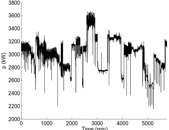
While small distributed PV has stimulated much of the research in this area, large and highly intermittent load or generation can create similar, or perhaps more difficult, voltage problems. One such example is a large (several MW) PV generator. However, the motivating example for us is a high-performance computing (HPC) load at Los Alamos National Lab. Power consumption of a modern HPC load can easily swing by several MWs in a few seconds or less, as shown by Fig. 1.1.

0 1000 2000 3000 4000 5000

2000 2200 2400 2600 2800 3000 3200 3400 3600 3800

Time (min)

[image:21.612.153.438.335.555.2]

p (kW)

Figure 1.1: A four-day real power consumption profile (sampled every five seconds) of the high performance computing load studied in this thesis.

(22)

on the current-stage average power, the probability distribution of the next-stage average power reveals information about the direction and size of voltage change that may occur in the next stage. We leverage this information to develop an improved voltage control scheme for distribution systems with large and rapid changes in load or generation. We then embed the proposed control into an optimal sizing problem for reactive power sources, which balances the capital cost of the devices with the expected cost due to power losses.

Specifically, the slow-timescale capacitor control is implemented by solving a chance-constrained optimal power flow (OPF) problem which minimizes power loss, regulates the current-stage voltage, and limits the probability of voltage viola-tions in the next stage. At the fast timescale, we control a D-STATCOM without loss of generality, by solving an OPF problem with deterministic constraints. The con-trol scheme above forms the basis of an optimal sizing problem, which determines the sizes of the two control devices above as well as a fixed capacitor to minimize the sum of the cost of expected power loss and the capital cost of all the devices. Exploiting structures of the chance-constrained OPF, we develop a computationally efficient heuristic based on simulated annealing to solve the sizing problem, and a heuristic for simpler real-time implementation of voltage control. Simulations on the realistic HPC load in Fig. 1.1 have shown that the proposed control and sizing schemes achieve a desired tradeoff between voltage safety and cost. In particular, voltage violations are significantly reduced with a moderate increase in cost.

1.3 Thesis outline

The rest of this thesis is organized as follows.

1. In Chapters 2 and 3 we design and analyze load-side distributed frequency control. Chapter 2 focuses on single-machine power systems [49], [50], [51], and Chapter 3 on multi-machine power networks. In Chapter 3, we work on the cases of load-side primary frequency control under a linearized power flow model [53], [54], and generator and load-side primary [55] and secondary [56] frequency controls under a nonlinear power network model. We also design a completely decentralized frequency integral control, as well as a distributed averaging-based proportional integral control [59].

(23)

C h a p t e r 2

LOAD-SIDE FREQUENCY CONTROL IN SINGLE-MACHINE

SYSTEMS

We consider a dynamically coherent power system that can be equivalently modeled with a single synchronous machine connected to a group of loads. We propose a decentralized load-side frequency control scheme that stabilizes frequency after a sudden change in generation or load. The proposed scheme exploits flexibil-ity of frequency responsive loads and neighborhood area communication to solve an optimal load control (OLC) problem that rebalances load and generation while minimizing end-use disutility of participating in load control. Local frequency measurements enable individual loads to estimate the mismatch between load and generation across the whole system. Neighborhood area communication alleviates performance degradation caused by frequency measurement noise. We also ana-lyze convergence of the proposed scheme under asynchronous measurements and actuations with bounded time delays. Simulations show that the proposed scheme is robust to model inaccuracies, and its performance is scalable with the number of participating loads. Moreover, a moderate amount of neighborhood communication is enough to achieve significant performance improvement.

This chapter is organized as follows. Section 2.1 introduces the power system model and formulates the OLC problem. Section 2.2 introduces the approach of estimating total load-generation mismatch from local frequency measurements, a key part of our control algorithm. Section 2.3 presents the decentralized load-side frequency control algorithm and proves its convergence. Section 2.4 proves convergence of the decentralized load-side frequency control under asynchronous measurements and actuations. Section 2.5 shows simulation results. Finally, Section 2.6 concludes this chapter. The proofs of propositions, theorems, etc. are provided in the Appendices.

2.1 System model and problem formulation

(24)

1

d



g



Generation control

1    

3

d

 d_N

 

3

+

 

  + N

Generation

2

d



2

+

  

1

N d _



1

+ N

   

Household appliances

Data center Electric vehicles

Commercial building

Industrial load

[image:24.612.140.470.75.292.2]

Loads

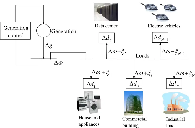
Figure 2.1: The single-machine power system model where∆gdenotes a generation drop and∆ω denotes the frequency deviation. Loadiobtains a measured value of the frequency deviation which may differ from∆ω by a stochastic noise ξi. Based on the measured frequency deviation, loadiis reduced by∆di.

Power system model

We consider the power system model in Fig. 2.1. We assume that the electrical distances between geographically different parts of the system are negligible, and so are the differences in frequencies between them [52]. Therefore, the whole system has a universal frequency which can be equivalently regarded as the frequency of a single generator. A number of controllable loads are connected to the generator and consume the generated power. A controllable load may also be an aggregate of multiple, smaller controllable loads [9][24].

LetV = {1,2, . . . ,N} denote the set of loads. Suppose the system is working at an operating point where the total load and generation are balanced. Then suddenly a generation drop denoted by ∆g occurs. To compensate for∆g, loadi is reduced by∆dithrough load control to be designed. Let∆ωdenote the universal frequency deviation from its nominal value. Loadimeasures the frequency deviation locally, and gets a measured value∆ωi, which may differ from∆ω by a stochastic noiseξi.

(25)

stand for the reduction of loadi at timet. Then, the total mismatch between load and generation at timetis

u(t) :=− X

i=1,...,N

∆di(t)+∆g(t). (2.1)

Without loss of generality, we let∆di(t) > 0 denote load reduction and∆g(t) > 0 generation drop, and therefore u(t) is the load surplus. We consider a dynamic model of the power system, which takes u as the input and ∆ω and ∆ωi as the output. To simplify the analysis, we use a linearized model around the operating point [14], [16]. Let x(t) ∈ _Rn denote the system state at time t. The elements in x depend on the specific power system model used in the algorithm. For example, they may include the valve position of the turbine, the mechanic power and the output voltage of the generator, and the frequency deviation ∆ω. We consider a stochastic disturbance to system state caused by environmental factors, e.g., change in temperature [87]. Such a disturbance is denoted byζ ∈_Rn. Moreover, for every loadi, the stochastic frequency measurement noiseξiis also considered. Then, the power system dynamic model is

x(t+1)= Ax(t)+Bu(t)+ζ(t), ∆ω(t)=C x(t),

∆ωi(t)= ∆ω(t)+ξi(t).

(2.2)

In this model, the frequency deviation∆ωis one element in the statex, and therefore the matrixC ∈_R1×nhas one element 1 and other elements 0.

We assume, for allt,s ≥ 0 and alli,j ∈ V, that the process disturbanceζ and the measurement noiseξihave zero mean, and are uncorrelated spatially and temporally and with each other, i.e., their covariances satisfy

E

f

ζ(t)ζ(s)Tg =Qδt s,

E

f

ξi(t)ξj(s)

g

=Wδt sδi j,

(2.3)

where Q ∈ _Rn×n is positive semi-definite, W ≥ 0, and δt s and δi j denote the Kronecker delta function. Here we assume that every load performs frequency mea-surement independently at every time step, so the meamea-surement noise is independent across the loads and not correlated over time. Moreover, we assume the noises at different loads have the same variance.

(26)

a single generator. In Chapter 3, we model such a system as a network of multiple generators connected by transmission lines. In the multi-machine model, we mainly focus on the effects of network structure on load control; therefore, we will consider a simple swing dynamic model of generators, in contrast to the more general model in (2.2). We also ignore the process disturbance and the measurement noise for multi-machine networks. In the current chapter, however, we focus on capturing the underlying dynamics in more detail.

Optimal load control

Without loss of generality, suppose the generation drops by a positive constant∆g at time 0. In response, loadi will be reduced by∆di(t) for t ≥ 0. As t → ∞, we want∆di(t) to converge to some∆d∗_i ∈[0,di], wherediis the maximum reduction of loadiallowed by appliance specification or user preference. Moreover, we desire

∆d_i∗to be an optimal solution to the following optimization problem:

OLC (single machine):

min

∆di∈[0,di]

N

X

i=1

ci(∆di)

subject to ∆g−

N

X

i=1

∆di =0,

(2.4)

whereci(∆di)is thedisutilitydue to interrupting the normal usage and compromising the end-use function of appliances [9][28]. By solving OLC (2.4), the total load and generation is rebalanced, which essentially stabilizes and restores the frequency to its nominal value, in a manner that minimizes the total end-use disutility.

For feasibility of OLC, we assume PN

i=1di −∆g > 0. This assumption holds if a large enough group of loads participate in frequency control. We make the following assumptions on the disutility functionscisuch that OLC is a convex problem.

Assumption 2.1. For alli = 1, . . . ,N, the functionci is increasing, strictly convex, and twice continuously differentiable, on [0,di].

Assumption2.2. For alli= 1, . . . ,N, there existsαi > 0, such thatc00_i (∆di) ≥ 1/αi for all∆di ∈[0,di]. Letα:=maxi₌₁,...,Nαi.

(27)

Solving OLC using a traditional centralized scheme requires a control center and two-way communication between the loads and the center: load-to-center com-munication to collect information like disutility functions and capacities of load reduction, and center-to-load communication to send the control signals ∆di(t). This centralized scheme has the following limitations in implementation. First, it requires the center to maintain connections with all the loads and perform com-putation for the whole system-level problem. If a fault occurs to the center or the communication infrastructure, the whole system control function may fail. Second, due to privacy issues, the users may not want to reveal information about their power usage to the system operator in the control center.

As an alternative, we design a more robust, scalable, and privacy-preserving decen-tralized scheme where every load computes a small piece of the overall problem, and exchanges information with a small number of its neighbors. For the purpose of such a design, we consider solving the dual problem of OLC. Taking pas the dual variable, the dual problem of OLC is

max p∈R

Ψ(p) := N

X

i=1

Ψi(p)+p∆g (2.5)

where

Ψi(p) := min

∆di∈[0,di]

ci(∆di)−p∆di. (2.6)

Under Assumption 2.1, givenp∈_R, the problem

min

∆di∈[0,di]

ci(∆di)−p∆di (2.7)

has a unique minimizer

∆di(p) =min(max{(c_i0)−1(p),0},di). (2.8)

Note that the inverse function ofc0_i exists over [c_i0(0),c_i0(di)] sincec_i0is continuous and strictly increasing by Assumption 2.1. Since ci is convex for alli = 1, . . . ,N and OLC has affine constraints, Slater’s condition implies that there is zero duality gap between OLC and its dual (2.5), and the optimal solution of (2.5), denoted by p∗, is attained [93, Sec. 5.5.3]. It follows that∆d(p∗) := [∆d1(p∗), . . . ,∆dN(p∗)]T is primal feasible and optimal [93, Sec. 5.5.2]. Moreover, it is easy to show that, for any given p and p such that p ≤ min

i c

0

i(0) and p ≥ max_i c

0

(28)

(2.5) has at least one optimal pointp∗ ∈[p,p]. Hence, we can constrain pto [p,p]. Therefore, instead of solving OLC directly, we solve its modified dual problem

Dual OLC:

max

p∈[p,p] Ψ(p) = N

X

i=1

Ψi(p)+p∆g. (2.9)

Informally, the decentralized algorithm is as follows (see Section 2.3 for a formal treatment). Each loadiupdates its value of dual variablepat timet as

pi(t) = max(min{pi(t−1)+γ(t)u(t−1),p},p), (2.10)

where γ(t) > 0 is some stepsize, and u(t − 1) = ∆g − PN

i=1∆di(t − 1) is the mismatch between load and generation at time (t −1). Then, loadi calculates its load reduction at timetas∆di(t)= ∆di(pi(t)),1where∆di(·)is defined in (2.8). It can be observed from (2.5)–(2.6) thatu(t −1)is the gradient of the dual objective functionΨin (2.9), if the dual variablep= p1(t−1)= · · ·= pN(t−1). Therefore, this decentralized algorithm is essentially a gradient projection method [93] applied to Dual OLC. To implement this algorithm with frequency responsive loads, loads should be able to estimateu from local frequency measurements. Our estimation method is introduced in the next section.

2.2 Estimating load-generation mismatch

In Section 2.1, we informally introduced a decentralized algorithm to solve the optimal load control problem OLC. The algorithm requires every load to know u = ∆g − PN

i=1∆di, the total mismatch between load and generation. We now introduce a method for individual loads to estimateu from local measurements of frequency deviation. Sinceuis the input to the state-space model (2.2), we call this methodinput estimation.

In input estimation, load i uses frequency measurements ∆ωi(1), . . . ,∆ωi(t) to estimateu(0), . . . ,u(t−1). In (2.2), we use ˆxi(t|s)and ˆui(t|s)respectively to denote the estimates of x(t) andu(t)with frequency measurements up to time s. Starting from ˆxi(1|0), the input estimation is recursively [94]:

ˆ

ui(t−1|t) = M ∆ωi(t)−Cxiˆ (t|t−1), ˆ

xi(t|t) = xiˆ (t|t−1)+Buiˆ (t−1|t),

ˆ

xi(t+1|t) = Axiˆ (t|t),

(2.11)

1_{We abuse notation by letting}_∆_d

(29)

where M := (C B)−1. Note that B ∈ _Rn×1 and both u(t) and C B are scalars. Therefore we only need the following assumption to ensure the existence of M.

Assumption2.3. The matricesCand BsatisfyC B_,0.

Assumption 2.3 holds for many practical power systems, including the one we will use in the case studies in Section 2.5.

The input estimation (2.11) gives an unbiased and minimum variance estimate of the state and the input. The covariance of xi(t|t), denoted byΣi_t_|_t ∈ _Rn×n, is given recursively by

Σ_ti₊₁_|_t₊₁ = (In−B MC)(AΣ_ti_|_tAT +Q)(In−B MC)T +B MW MTBT,(2.12)

where Q and W are defined in (2.3). Denote the input estimate error by ei(t) := ˆ

ui(t|t+1)−u(t). Define theσ-algebraFt−1:= σ(ei(τ−1);i =1, . . . ,N,1≤ τ≤ t) which includes the historical information before time t for all the loads. The expectation and variance ofei(t)conditioned onFt−1are [94]:

E[ei(t)|Ft−1] = 0 (2.13) and

E

f

(ei(t))2|F_t−1

g

= C AΣ

i t|tA

T

CT +W

(C B)2 . (2.14)

The following proposition provides a condition under whichE

f

(ei(t))2|Ft−1

g

con-verges to a constant ast → ∞.

Proposition2.1. Denote the eigenvalues of(In−B(C B)−1C)Abyλs, s= 1, . . . ,n. If|λs| <1 for all s=1, . . . ,n, then

lim t→∞E

f

(ei(t))2|Ft−1

g

= σ2

∞ (2.15)

whereσ2_∞is a constant determined by A, B,C,Q, andW, and independent ofi.

Proof. See Appendix 2.A.

For any power system model in the form of (2.2), we can check a priori whether the condition in Proposition 2.1 is satisfied. However, the implications of this condition still need to be understood in future studies.

(30)

Corollary2.1. If the condition for Proposition 2.1 holds, thenE

f

(ei(t))2|Ft−1

g ≤ σ2

for alli =1, . . . ,Nand allt ≥0, whereσ2is a constant which depends on A,B, C,Q,W, and the initial covarianceΣ₀i_|₀for alli =1, . . . ,N.

With the input estimation (2.11), every load can get a local estimate of u. The estimates of different loads i may not be the same, due to different realizations of measurement noiseξifor differenti. By (2.10), the inconsistencies of estimates ofu lead to inconsistencies ofpibetween different loadsi. However, in the decentralized algorithm informally given in Section 2.1, we desire pi to converge to the optimal point of Dual OLC for alli= 1, . . . ,N. Therefore, the inconsistencies ofpibetween the loads should be eliminated or mitigated. In Section 2.3 below, we will introduce a method to mitigate such inconsistencies. Then, we will formally propose the decentralized load control algorithm and prove its convergence.

2.3 Decentralized load control: algorithm and convergence

In this section, we introduce a method to mitigate the inconsistencies ofpi between different loads, and describe formally the decentralized, frequency-based algorithm that solves the optimal load control problem OLC. Then, we discuss the communi-cation architecture that supports this algorithm. We also present convergence results of the proposed algorithm.

Decentralized load control algorithm

The decentralized algorithm was informally discussed in Section 2.1. The dual variable update in (2.10) requires estimating u locally. As shown in Section 2.2, there may be inconsistencies between local estimates ofu, and hence between pi, for different loadsi.

We use neighborhood communication between the loads to mitigate such incon-sistencies. The information flow of such communication can be regarded as an undirected graph, since the communication is in two ways. In this graph, denote the set of neighbors of loadiat timet asN(i,t). Loadiis assigned a weightri j(t) for all j ∈ N(i,t), and a weightrii(t)for itself. Note that if j ∈ N(i,t)theni ∈ N(j,t). We makeri j(t) =rji(t), and can always find the weights that satisfy

X

j=i,j∈N(i,t)

ri j(t)= 1, X j=i,j∈N(i,t)

rji(t)= 1. (2.16)

(31)

from all j ∈ N(i,t), and calculates their average value, denoted byqi(t), as

qi(t) = X

j=i,j∈N(i,t)

ri j(t)pj(t). (2.17)

This averaging procedure is typically used in consensus algorithms [95]. Consensus, in our problem, means that the loads seek agreement on the values of the dual variable p. In (2.17),qi is an auxiliary variable which denotes a local average of the values of the dual variable across loadiand its neighbors. As the algorithm iterates, this local averaging propagates to a global agreement on the values of the dual variable throughout the network. Combining such a consensus procedure with the estimation of u in Section 2.2, we have the following decentralized algorithm to solve OLC (2.4) and its dual (2.9).

Algorithm 2.1. Decentralized load-side frequency control for single-machine sys-tems

At time t = 0, the following information is known to all loadsi = 1, . . . ,N: the matrices A, B andC in system model (2.2), the lower bound p and upper bound

p defined in Section 2.1, and a sequence of positive stepsizes {γ(t),t = 1,2, . . .}

which is the same for all the loads. Each loadi starts from an arbitrary initial state estimate ˆxi(1|0)and an initial value of dual variableqi(0).

At time instantst = 1,2, . . ., every loadi:

1. Measures the frequency deviation∆ωi(t), and calculates ˆui(t−1|t)using the input estimation (2.11).

2. Updates the value of dual variable according to

pi(t) = max(min{qi(t−1)+γ(t)uiˆ (t−1|t),p},p) (2.18)

and transmitspi(t)to all of its neighbors j ∈ N(i,t).

3. Receives thepj(t)from all j ∈ N(i,t), and calculatesqi(t)as (2.17).

4. Computes load reduction∆di(t) =∆di(qi(t))where∆di(·)is defined in (2.8).

(32)

Neighborhood area communication

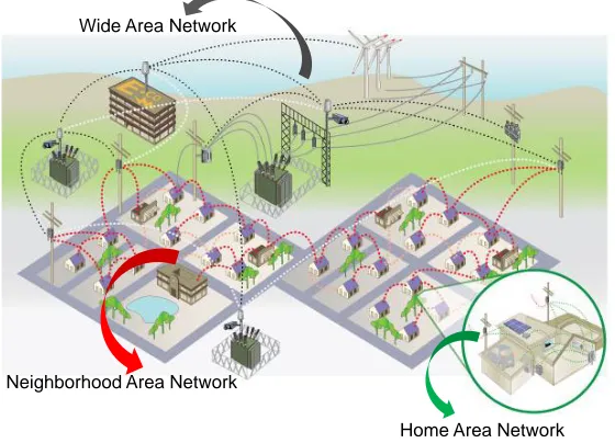
As an example, we take the smart grid communication architecture proposed by Trilliant, Inc. [96] shown in Fig. 2.2.

Wide Area Network

Neighborhood Area Network

[image:32.612.167.447.143.345.2]

Home Area Network

Figure 2.2: The home area network (HAN) supports the communication between appliances and smart meters. The neighborhood area network (NAN), which is used in our load control, aids the communication between utilities and smart meters. The wide area network (WAN) aids the long range communication between substations. This figure is a slightly modified version of a similar figure in [96].

The load control scheme given by Algorithm 2.1 does not rely on communication between all the loads and a control center. Instead, it uses communication between each load and its neighbors. This neighborhood communication uses mainly a neighborhood area network (NAN). In NAN, reliable, scalable, fast responding and cost-effective communication technologies such as 802.2.15.4/ZigBee are widely used to facilitate the implementation of the decentralized load control.

For the convergence proof of Algorithm 2.1, we make the following assumption on the weightsri j(t)in (2.17).

Assumption 2.4. There exists a scalar 0 < η < 1 such that for alli = 1, . . . ,N and allt ≥ 0, we haveri j(t) ≥ ηif j =ior j ∈ N(i,t), andri j(t) =0 otherwise.

With Assumption 2.4, equation (2.17) simplifies to

qi(t) =

N

X

j=1

(33)

Moreover, in order to make the information at loadjaffect loadiinfinitely often, we assume that within any fixed period of time, the set of communication links which have appeared form a connected, undirected graph. DefineEt := {(i,j)|ri j(t) > 0}

to be the set of undirected links at timet. The connectivity requirement above is formally stated in the following assumption.

Assumption2.5. There exists a integerQ ≥ 1 such that the graph(V, S τ=1,...,Q

Et₊τ−1) is connected for allt.

In reality, the NAN may have specific topologies, e.g., bus, ring, star, linear topol-ogy, or mixed topologies, as discussed in [97], [98]. All these topologies satisfy Assumption 2.5. However, the convergence analysis does not require any additional assumptions on the topology beyond Assumption 2.5. We will consider a realistic topology in case studies in Section 2.5.

DefineR(t)to be the matrix with(i,j)-th entryri j(t), and defineΦ(t,s) := R(t)R(t−

1). . .R(s+1). The following result given by [95, Lemma 3.2] will be used in the convergence proof of Algorithm 2.1:

[Φ(t,s)]i j − 1

N

≤ θ βt−s, (2.20)

where

θ = 1− η

4N2

−2

, β = 1− η

4N2

_Q1

. (2.21)

Convergence of Algorithm 2.1

Now we present results regarding the convergence of Algorithm 2.1. We first consider the case where the sequence {γ(t),t = 1,2, . . .}of stepsizes converges to some nonnegative constant. Theorem 2.1 gives a bound on the difference between the maximal expected value of the dual objective functionΨand the optimal value of Dual OLC, denoted byΨ∗.

Theorem 2.1. Suppose Assumptions 2.1–2.5 hold. If lim

t→∞γ(t) = γ ≥ 0 and ∞

P

t=1

γ(t)= ∞, then, for alli= 1, . . . ,N,

lim sup t→∞ E

[Ψ(pi(t))]≥ Ψ∗− γ(G

2₊_σ2

)

2 −γG(αN L+G) 2+ Nθ β 1− β

!

, (2.22)

where G := max

( N P

i=1

di−∆g

,|∆g|

)

, σ is the bound on input estimate error in

(34)

Proof. See Appendix 2.B.

Taking γ = 0 in (2.22), we have the following corollary, which is straightforward from Theorem 2.1.

Corollary2.2. Suppose Assumptions 2.1–2.5 hold. If lim

t→∞γ(t) = 0 and ∞ P

t=1

γ(t) = ∞, then, for alli= 1, . . . ,N,

lim sup t→∞ E

_Ψ

pi(t) = Ψ∗.

Define ∆d(t) = [∆d1(t), . . . ,∆dN(t)]T. With further restrictions on the stepsize

γ(t), the sequence {∆d(t), t = 1,2, . . .} produced by Algorithm 2.1 converges almost surely to the optimal point of OLC, as stated in Theorem 2.2.

Theorem 2.2. Suppose Assumptions 2.1–2.5 hold,

∞ P

t=1

γ(t) =∞, and

∞ P

t=1

γ(t)2< ∞. Then, for alli =1, . . . ,N, the sequence{qi(t)}converges to the same optimal point of Dual OLC with probability 1 and in mean square. Moreover, the sequence{∆d(t)}

converges to the optimal point of OLC with probability 1.

Proof. See Appendix 2.C.

In Algorithm 2.1, neighborhood communication is used to mitigate the effect of measurement noise. Now we consider a special case where the process disturbance

ζ and the measurement noise ξi for all i = 1, . . . ,N are zero. In this case, the following theorem shows that OLC can be solved by using a simplified version of Algorithm 2.1 which does not need neighborhood communication.

Theorem 2.3. Suppose Assumptions 2.1–2.3 hold, and the following conditions are satisfied:

1. ζ(t) =0 andξi(t) =0 for alli= 1, . . . ,N andt ≥ 0.

2. In Algorithm 2.1, for alli =1, . . . ,N, ˆxi(1|0)= x(1), andqi(0)are the same.

3. For alli =1, . . . ,N and allt ≥0,rii(t)= 1, andN(i,t) =∅.

4. Constant stepsizeγ(t) = γ, whereγ satisfies 0< γ < 2/(αN), is used.

Then, for all i = 1, . . . ,N, any limit point (at least one exists) of the sequence

{ ∆d(t),qi(t),

(35)

Proof. See Appendix 2.D.

The algorithm and convergence proof above are based on an underlying assumption that all the loads simultaneously and synchronously measure their local frequency deviations and take control actions. In practice, this is obviously not the case. In the next section we will investigate convergence of the proposed scheme under asynchronous measurements and actuations with bounded time delays.

2.4 Asynchronous measurements and actuations

In this section, we ignore stochastic process disturbance and measurement noise, by assumingζ(t) =0 and ξi(t)= 0 for alli =1, . . . ,N andt ≥ 0.

In the asynchronous setting, the frequency deviation∆ω(t) at time t is accurately measured by load i = 1, . . . ,N at some time within the interval [t + r(i,t) −

1,t +r(i,t)), where r(i,t) ∈ _N is an arbitrary fixed number. In the time inter-val [t − 1,t), load i measures a set of frequency deviation signals, denoted by

Ωi,t = {∆ωˆ_i1_,_t, ...,∆ωˆ Ki,t

i,t }, where Ki,t is the number of measured frequency deviation samples (Ωi,t = ∅ and Ki,t = 0 means no frequency deviation signal is measured during [t−1,t)). Moreover, loadiis able to change its power only at a subset of time instants, denoted byTi ⊆ {0,1,2, . . .}. For the asynchronous algorithm to converge, we make the following assumptions onr(i,t)andTi.

Assumption 2.6. For alli = 1, . . . ,N, t ≥ 0, l ∈ {1, . . . ,Ki,t} and s ∈ {1, . . . ,t}, if ∆ωˆ_il_,_t is the measurement of ∆ωs, then ∆ωˆ_il_,+1_t is the measurement of ∆ωs+1. Moreover, there existsr ∈_Nsuch thatr(i,t) ≤ r for alli =1, . . . ,N andt ≥ 0. Assumption 2.7. For alli = 1, . . . ,N, the difference between any two consecutive elements inTiis bounded.

Assumption 2.6 says that the delayed frequency measurements arrive in order. In other words, the frequency deviation signal that occurs first is sensed first by the load. Moreover, the time delays in frequency measurement are bounded by r. Assumption 2.7 says that the time between any consecutive change of any load is bounded.

With the settings above, we present the asynchronous algorithm as follows.

(36)

Suppose all loadsi= 1, . . . ,Nknow the matrices A, BandCin system model (2.2). Choose the same stepsizeγ >0 for all of them. At timet =0, initialize each loadi with ˆxi₀= x(0),₂and pi(0) =0.

In the time interval [t−1,t)fort =1,2, . . ., every loadi:

1. At time(t−1), sets ˆxi_t₋₁(0|0) = xˆi_t₋₁, pi_t₋₁(0) = pi(t−1).

2. Once load i measures a new frequency deviation signal ∆ωˆ_ik_,_t ∈ Ωi,t for k =1, . . . ,Ki,t, it calculates ˆui_t₋₁(k)by

ˆ

xi_t₋₁(k|k−1) = Axˆi_t₋₁(k−1|k −1),

ˆ

ui_t₋₁(k) = (C B)−1(∆ωˆ_ik_,_t −Cxˆi_t₋₁(k|k−1)),

ˆ

xi_t₋₁(k|k) = xˆi_t₋₁(k|k−1)+ Buˆi_t₋₁(k),

(2.23)

and updates the value ofpby

pi_t₋₁(k) = pi_t₋₁(k−1)+γuˆi_t₋₁(k). (2.24)

3. At timet, sets ˆxi_t = xˆ_ti₋₁(Ki,t|Ki,t) andpi(t) = p_ti₋₁(Ki,t).

4. If loadi is able to change its power at timet, i.e., ift ∈Ti, it determines this change as ∆di(t) = ∆di(pi(t)) where ∆di(·) is defined in (2.8); otherwise,

∆di(t) =∆di(t−1).

The following theorem states the convergence of Algorithm 2.2.

Theorem 2.4. Suppose Assumptions 2.1–2.3, 2.6, and 2.7 hold, and the stepsizeγ satisfies

0 < γ < 1

αN/2+2r.

Then for all i = 1, . . . ,N, any limit point (at least one exists) of the sequence

{ ∆d(t),pi(t),

t =1,2, . . .}is primal-dual optimal for OLC and Dual OLC.

Proof. See Appendix 2.E.

(37)

2.5 Simulations

We take a relatively detailed example of the power system model introduced in (2.2) for simulation-based experiments. We use Algorithm 2.1 to control the loads when a sudden generation drop occurs, and observe frequency, load reduction and total end-use disutility to evaluate its performance. Additionally, we test the robustness of Algorithm 2.1 to model inaccuracies by letting the loads use a simplified, less accurate model to estimate the mismatch between total load and generation. We also discuss tradeoffs between the amount of communication and the performance of the proposed scheme, and the effect of the number of participating loads.

System settings

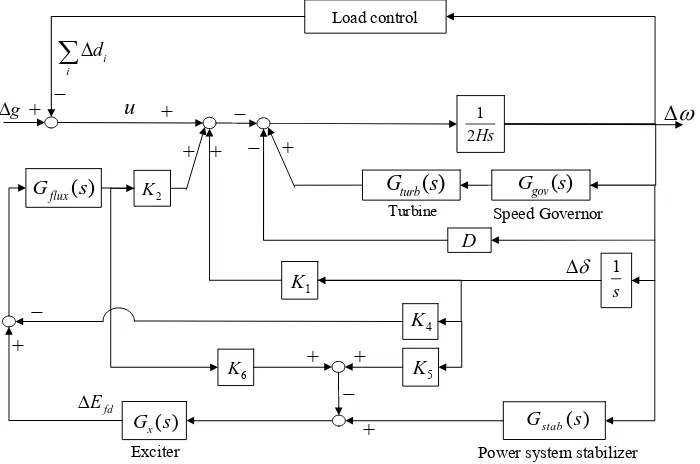
We consider an example of the single generator model (2.2), as shown in Fig. 2.3.

  g  u Exciter fd E  2 K Load control 1 K 4 K 5 K 6 K 1 s   i i d 



− ( ) flux G s [image:37.612.130.480.297.529.2]

Power system stabilizer ( ) stab G s + − + + + + ( ) x G s + Speed Governor Turbine + − D 1 2Hs ( ) gov G s ( ) turb G s + − − +

Figure 2.3: A single-machine power system model used in simulations.

This generator has a speed governor with the transfer function

Ggov(s) = −

1 R(1+sTG),

a turbine with the transfer function

Gtur b(s) = (1+sFH PTRH) (1+sTC H)(1+sTRH),

and a power system stabilizer (PSS) with the transfer function

Gstab(s) = sKw(1+sT1)(1+sT3) (1+sTw)(1+sT2)(1+sT4)

(38)

The output voltage of the generator is regulated by an IEEE AC4A exciter [14], which has the transfer function

Gx(s) =

KA(1+sTC)

(1+sTA)(1+sTB).

Moreover, the flux decay transfer function of the generator is

Gf lux(s) =

[image:38.612.150.461.238.430.2]

K3 1+K3τ_d00 s.

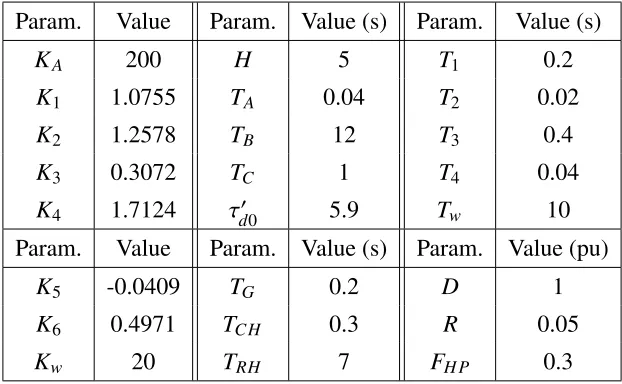
Table 2.1 gives the values of parameters used in the transfer functions above.

Param. Value Param. Value (s) Param. Value (s)

KA 200 H 5 T1 0.2

K1 1.0755 TA 0.04 T2 0.02

K2 1.2578 TB 12 T3 0.4

K3 0.3072 TC 1 T4 0.04

K4 1.7124 τ_d00 5.9 Tw 10

Param. Value Param. Value (s) Param. Value (pu)

K5 -0.0409 TG 0.2 D 1

K6 0.4971 TC H 0.3 R 0.05

Kw 20 TRH 7 FH P 0.3

Table 2.1: Parameters used in the simulations of the single-machine system.

The continuous-time state-space form of the model above is

˙

x = Acx+Bcu,

∆ω =Ccx.

Then, taking a sample time∆t = 0.5 s, we get the matricesA,BandCin (2.2) using the following equations:

A= eAc∆t,

B= A−_c1(A−In)Bc, C =Cc.

(39)

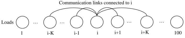
i-1 i i+1 i+K 100

… …

i-K … …

1 Loads

[image:39.612.127.481.74.148.2]

Communication links connected to i

Figure 2.4: An example communication graph of loads.

Loadi has a disutility functionci(∆di) = (∆di)2/(2αi). In this section, we pickαi subject to the uniform distribution on [1,3]. The baseline power isPbase =200 MVA. Fori = 1, . . . ,N, we have∆di ∈[0,di]. We choosedi to be positive numbers such thatPN

i=1di = 0.30 per unit (pu). Generation drop∆g(t) makes two step changes resembling sudden generation loss events:

∆g(t) =               

0 0 ≤t <20 s

0.05 pu 20 s ≤ t < 50 s

0.15 pu t ≥ 50 s.

The process disturbanceζhas covarianceQ = B(0.002 pu)2BTforBobtained above. The measurement noise ξi for alli = 1, . . . ,N has variance W = (0.001 pu)2. In Algorithm 2.1, all the loads use a diminishing stepsizeγ(t) = γ(0)/(t0.8)for some arbitrarily selectedγ(0) > 0, so thatP∞_t₌₁γ(t) =∞andP∞_t₌₁γ(t)2 < ∞. Therefore, all the conditions in Theorems 2.1 and 2.2 are satisfied.

Robustness to model inaccuracies

We compare the performance of the load control scheme Algorithm 2.1 between the two settings: “accurate modeling” and “simplified modeling.” Under accurate modeling, loads use the accurate model given by matrices A, B and C for input estimation. Under simplified modeling, loads use a simplified, less accurate model, due to the practical consideration that the system operator or utility company may not reveal the exact system information to users because of privacy issues. There are multiple ways to simplify the system model. For example, in the model given by Fig. 2.3, we consider the swing dynamics only and ignore all the other parts, and, with the values of parameters given in Table 2.1, we have a simplified transfer function

H

G(s) = − 0.1555s+0.0222

s2+0.9918s+0.4666

(40)

Figs. 2.5–2.7 respectively show the frequency, the total load reduction and the total end-use disutility with loads using different models. There are N = 100 loads, and every load communicates withK =5 neighbors (except the loads at the two ends of the linear graph in Fig. 2.4).

20 30 40 50 60 70 80

59.6 59.8 60 60.2

t: Time (sec)

Frequency (Hz)

[image:40.612.176.423.443.632.2]

no load control accurate model simplified model

Figure 2.5: The frequency (N=100, K=5). The dash-dot line is the frequency without load control. The solid and dashed lines are those with load control where loads use different models.

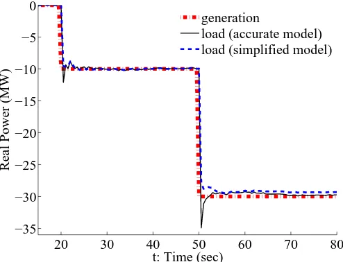
20 30 40 50 60 70 80

−35 −30 −25 −20 −15 −10 −5 0

t: Time (sec)

Real Power (MW)

generation

load (accurate model) load (simplified model)

(41)

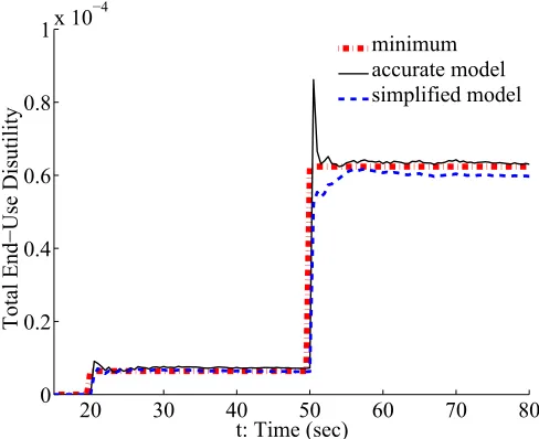
20 30 40 50 60 70 80 0

0.2 0.4 0.6 0.8

1x 10−4

t: Time (sec)

Total End−Use Disutility

[image:41.612.179.423.74.273.2]

minimum accurate model simplified model

Figure 2.7: The total end-use disutility (N=100, K=5). The dash-dot line is the minimal disutility. The solid and dashed lines are trajectories of the disutility with load control where loads use different models.

In both scenarios of load control using different models, the frequency is recovered to 60 Hz faster than in the case without load control. The total load reduction follows the generation drop, and the total end-use disutility converges to the minimum, both within a short time. It takes 7 iterations (3.5 seconds) for the disutility to achieve and stay within±5% of the new steady-state (minimum) value after the first generation drop, and 8 iterations (4 seconds) after the second. Moreover, all the results under the simplified model are close to those under the accurate model, which suggests the proposed scheme is robust to model inaccuracies considered here.

Tradeoffs between communication and performance

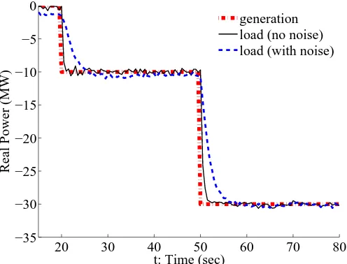
Theorem 2.3 states the convergence of Algorithm 2.1 without communication be-tween loads, when there is no process disturbance or measurement noise in the system. Otherwise, communication is required to guarantee satisfactory perfor-mance of the proposed scheme. To demonstrate this, Figs. 2.8–2.10 respectively show the frequency, the total load reduction and the total end-use disutility when loads perform Algorithm 2.1 withK = 0, i.e., no communication between the loads. Constant stepsizeγ = 1.4/(αN)is used to satisfy the condition in Theorem 2.3.

(42)

20 30 40 50 60 70 80 59.5

59.6 59.7 59.8 59.9 60 60.1 60.2 60.3

t: Time (sec)

Frequency (Hz)

[image:42.612.176.424.366.555.2]

no load control load control (no noise) load control (with noise)

Figure 2.8: The frequency when there is no communication in load control (N=100, K=0). The dash-dot line is the frequency without load control. The solid and dashed lines are respectively the frequencies without and with measurement noise in load control.

20 30 40 50 60 70 80

−35 −30 −25 −20 −15 −10 −5 0

t: Time (sec)

Real Power (MW)

generation load (no noise) load (with noise)

Figure 2.9: The total load reduction when there is no communication in load control (N=100, K=0). The dash-dot line is the generation drop. The solid and dashed lines are respectively the load reductions without and with measurement noise in load control.

without communication. However, when there is measurement noise, Algorithm 2.1 produces a lower nadir in frequency, a larger delay in load adjustment, and a disutility much higher than the minimum.

(43)

per-20 30 40 50 60 70 80 0

0.5 1 1.5

x 10−4

t: Time (sec)

[image:43.612.180.422.73.273.2]

minimum no noise with noise

Figure 2.10: The total disutility when there is no communication in load control (N=100, K=0). The dash-dot line is the minimal disutility. The solid and dashed lines are respectively the disutility without and with measurement noise in load control.

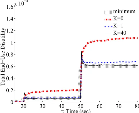
formance of Algorithm 2.1. In the communication graph we use, as K grows, the connectivity gets stronger and more communication is used. We show the total end-use disutility withK =0,1,40, in Fig. 2.11.

20 30 40 50 60 70 80

0 0.2 0.4 0.6 0.8 1 1.2 1.4 1.6x 10−4

t: Time (sec)

minimum K=0 K=1 K=40

Figure 2.11: The total end-use disutility with different numbers K of neighbors in the load control (N=100).

[image:43.612.179.421.431.627.2]

(44)

On the other hand, the results are significantly improved when K increases from 0 to 1, but not so distinguishable when increasingK from 5 to 40. It implies that the proposed scheme can effectively address frequency measurement noise, and receive most of its benefit, using a moderate amount of neighborhood communication.

Effects of the number of loads

We consider the effects of different numbers of loads that implement the decentral-ized load control Algorithm 2.1. Fig. 2.12 shows the total end-use disutility with N = 10, N =100, and N =1000. In all the three cases, every load communicates with the same number of neighborsK = 5. Moreover, the values of parameters in different cases are scaled so that they have the same minimal disutility.

20 30 40 50 60 70 80

0 2 4 6 8

x 10−5

t: Time (sec)

[image:44.612.186.421.281.478.2]

minimum N=10 N=100 N=1000

Figure 2.12: The total end-use disutility with different numbers N of loads (K=5).

We can see that the difference is negligible between different cases, which means the performance of the proposed scheme does not degrade as more and more loads participate. This result implies that the frequency-based, decentralized load control is suitable for large-scale deployment.

2.6 Conclusion

(45)

(46)

APPENDICES

2.A Proof of Proposition 2.1

Recall that M = (C B)−1. The matrix (In− B MC)Q(In− B MC)T + B MW MTBT is positive semi-definite, since both Q and W are positive semi-definite. Then, if

|λs|< 1 for alls =1, . . . ,n, the equation

Σ=(In−B MC)AΣAT(In−B MC)T

+(In−B MC)Q(In−B MC)T + B MW MTBT

has a unique, positive semi-definite solution Σ∗ [99]. Additionally, lim t→∞Σ

i

t|t exists and isΣ∗. By (2.14), we have

lim t→∞E

f

(ei(t))2|Ft−1

g

= C AΣ∗ATCT +W (C B)2 ,

where the right-hand-side is independent ofiand can be determined by A, B,C,Q, andW.

2.B Proof of Theorem 2.1

We first show two lemmas as a preparation for proving Theorem 2.1. Define y(t):= _N1 PN

i=1pi(t).

Lemma2.1. Suppose Assumptions 2.4 and 2.5 hold. Then for alli = 1, . . . ,N and t ≥ 0,

|y(t)−pi(t)| ≤θ βt

N

X

j=1

|pj(0)|+θ

t−1

X

τ=1

γ(τ)βt−τ

N

X

j=1

(G+ |e_τj₋₁|)

+ γ(t)

N N

X

j=1

Real-Time Load-Side Control of Electric Power Systems

Changhong Zhao

ORCID: 0000-0003-0539-8591

ACKNOWLEDGEMENTS

TABLE OF CONTENTS

LIST OF ILLUSTRATIONS

LIST OF TABLES

1.1 Distributed load-side frequency control

Summary of this work

1.2 Two-timescale voltage control

1.3 Thesis outline

LOAD-SIDE FREQUENCY CONTROL IN SINGLE-MACHINE

2.1 System model and problem formulation

Power system model

Optimal load control

Dual OLC:

2.2 Estimating load-generation mismatch

2.3 Decentralized load control: algorithm and convergence

Neighborhood area communication

Convergence of Algorithm 2.1

2.4 Asynchronous measurements and actuations

2.5 Simulations

Robustness to model inaccuracies

Tradeoffs between communication and performance

Effects of the number of loads

2.6 Conclusion

APPENDICES

2.A Proof of Proposition 2.1

2.B Proof of Theorem 2.1